3 Applications of Jacobian Matrix in Deep Learning and Robotics | Môn Linear algebra and Algebraic structures - Đại học Sư phạm Kỹ thuật Thành phố Hồ Chí Minh

lOMoAR cPSD| 58759230
3 Real-world applications of Jacobian Matrix
The Jacobian matrix is a fundamental concept in multivariate calculus, widely
recognized for its ability to describe how changes in multiple input variables affect
multiple output variables. This mathematical structure has numerous practical
applications across engineering, computer science, and artificial intelligence. In this
section, we will present some of its most impactful real-world applications, particularly
in deep learning and robotics.
3.1 Applications in Deep Learning
The Jacobian matrix is a fundamental mathematical tool, widely used in machine
learning and especially in deep learning. It provides a structured way to describe how
the output of a multivariable function changes with respect to its input. In deep neural
networks (DNNs), the Jacobian matrix plays a central role in model training,
optimization, and analysis, particularly in the implementation of backpropagation and in functions like Softmax.
3.1.1. The Softmax function in Deep Learning [1]
In deep learning models used for classification tasks, the Softmax function is a
mathematical tool used to convert raw output scores (logits) into a probability
distribution over the possible classes and it is defined as: ez i Softmax (zi) = n zk ∑ e k=1
Where n is the total number of classes. This transformation ensures that the
output values are in the range [0, 1] and sum up to 1, making them interpretable as class
probabilities. The class with the highest probability is selected as the model’s final prediction. lOMoAR cPSD| 58759230
For example, in a classification task involving four animals: dog, cat, and tiger,
suppose the input vector to Softmax is z = [2.5 1.0 3.0]. After applying Softmax, the
output probabilities will be σ= [0.35 0.08 0.57]. This means the model predicts a 35%
chance for “dog”, 8% for “cat” and 57% for “tiger”.
3.1.2. The role of Softmax function in training process [1, 2]
The main task during the training phase of a deep learning model is to minimize the
error between the prediction of the model (probabilities from Softmax) and the true
label. Like above example, if the true label is “dog”, the corresponding truth vector [1
0 0], the model uses a loss function (e.g., Cross-Entropy Loss) to measure the difference
between the predicted probabilities σ= [0.35 0.08 0.57] and the truth vector ytrue = [1
0 0]. To minimize this error, the input values to the Softmax function (known as logits)
must be adjusted so that the resulting output probabilities better match the true label. To
determine how changes in the logits affect the output probabilities, we can employ the
Jacobian matrix. This matrix captures the partial derivatives of each Softmax output
with respect to each logit input, providing essential information for the backpropagation
algorithm to compute the gradients needed for weight updates.
The below is representing how Jacobian matrix is formed in backpropagation of Softmax layer.
The Jacobian matrix J is the matrix of partial derivatives, where each element Jij is given by:
J ∂Softmax(zi) ij=¿ ¿ ∂( z j)
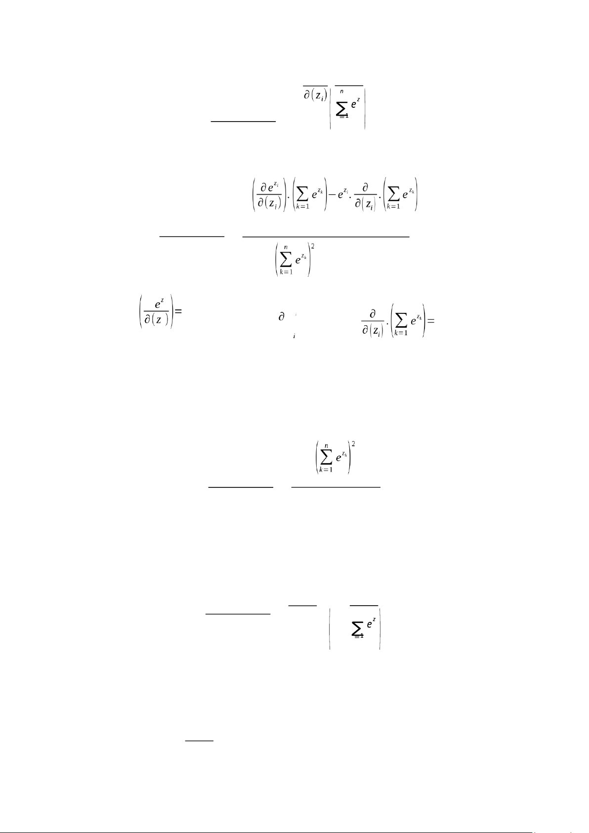
This matrix describes how each output of the Softmax function depends on its inputs. Derivative of Softmax Case 1: When i = j For i = j, we compute: lOMoAR cPSD| 58759230 ∂ ez i ∂Softmax(zi) k k ∂(zi) = Using the quotient rule: n n ∂Softmax(zi) ∂(zi) = n Since e zi and ezi , we get: n e )
zi .(∑= ez k −ezi .ez i ∂Softmax(zi) k 1 = ∂(zi) Then, we have
∂Softmax(zi) nezi 1− nezi k ∂(z . i) ∑ ez k k = k=1 ez i
Substitute σ = n , we get: i zk lOMoAR cPSD| 58759230 ∑ e k=1
∂(zi) = σ i(1−σi) (1)
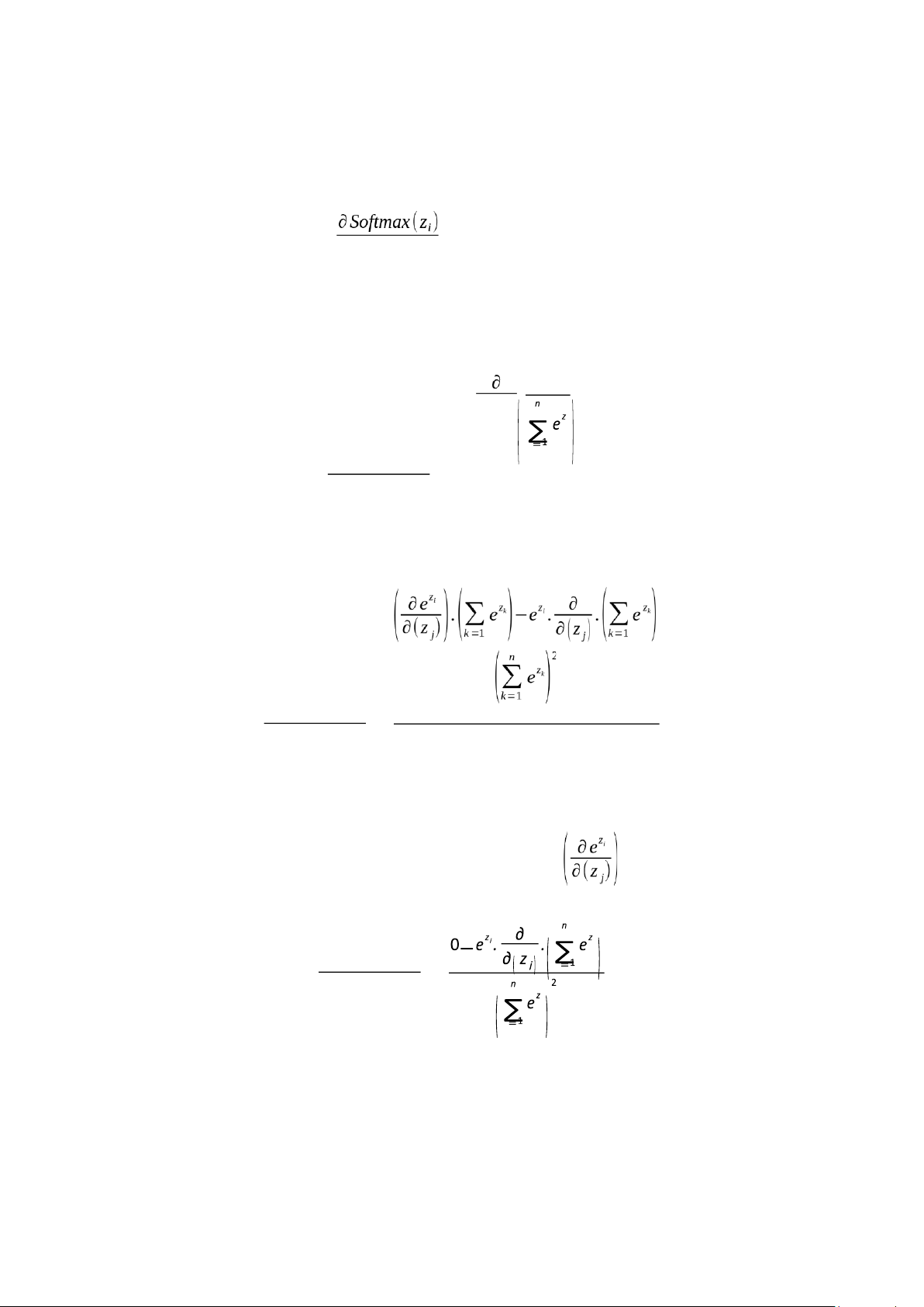
Case 2: When i ≠ j For i ≠ j, we compute: z e i k ∂Softmax(z i) k
∂(z j) = ∂(zj) Using the quotient rule: n n ∂Softmax(zi) = ∂(z j)
Because ez i is independent of z j, so its derivative =0 k k k k
∂Softmax(zi) = ∂(z j) lOMoAR cPSD| 58759230 n Since ez j , we get: −e z i .ezi
∂Softmax(zi) = k ∂(zi) k ez e i z j
Substitute σ i = n and we get: z σ k j = n zk ∑ e ∑ e k=1 k=1 ∂Softmax(zi)
∂(zi) = −σ i.σ j (2)
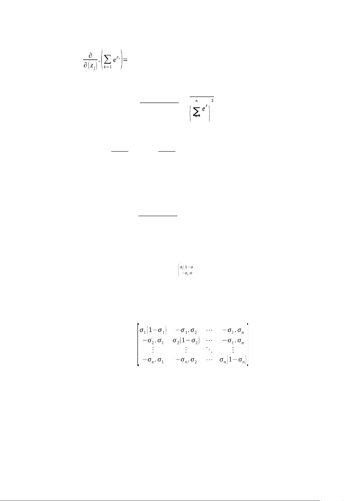
From (1) and (2), we can get the Jacobian matrix J for the Softmax function is: J )
ij=¿i ,if i=j¿ j ,if i≠ j
And the Jacobian Matrix Form J =
This Jacobian matrix is vital for computing gradients during backpropagation,
especially when the Softmax function is followed by a cross-entropy loss. It quantifies
how each logit affects every output probability, enabling the model to make the
necessary adjustments to minimize error. lOMoAR cPSD| 58759230
In the backpropagation process of training neural networks, the Jacobian matrix plays a
crucial role in determining how adjustments to the input values (logits) influence the
output probabilities produced by the Softmax function. Specifically, when there is an
error between the predicted output and the true labels, we aim to calculate the necessary
changes in the input that will reduce this error. This process involves two key steps.
First, the model computes the difference between the predicted probabilities and the
actual labels, denoted as Δy, which represents the desired change in the output. Second,
the Jacobian matrix of the Softmax function is used to map this output change back to
the required adjustment in the input logits, denoted as Δz. The relationship can be described by the formula: Δz = Δy x Jacobian
Δy quantifies the output error, and the Jacobian matrix provides the necessary
transformation to calculate how each logit should be adjusted to achieve the desired
change in output and ∆z is the required adjustment in the input (logits) to produce the
desired changes in the output.
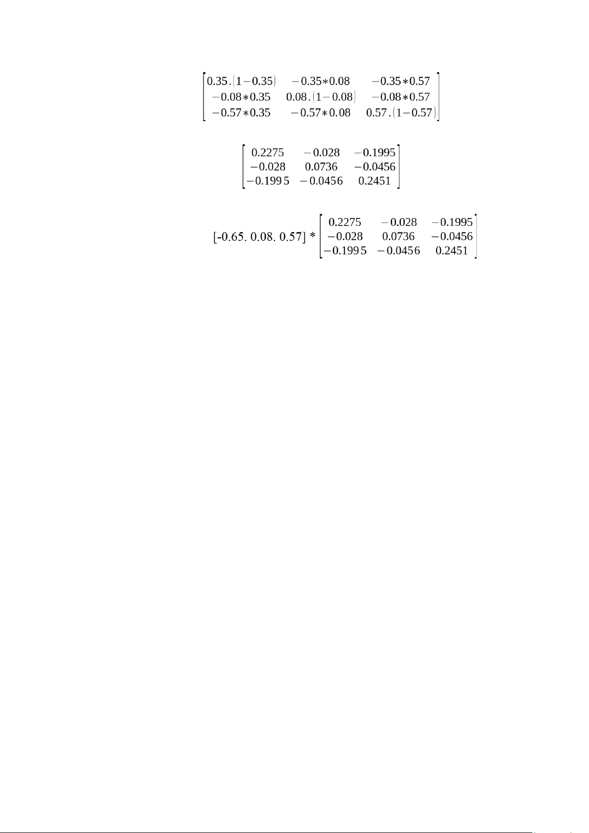
To better illustrate how the Jacobian matrix is applied during training, consider the
following numerical as above example: z = [2.5 1.0 3.0], σ= [0.35 0.08 0.57] and the truth vector ytrue = [1 0 0].
Then, the output error is Δy = σ - ytrue = [-0.65. 0.08. 0.57]
And the Jacobian Matrix Form of the Softmax function is: J =
Substitute the value in σ= [0.35 0.08 0.57] to matrix J, we get: lOMoAR cPSD| 58759230 J = J = Then Δz = Δy x Jacobian =
=> Δz = [-0.26. 0.0019 0.2657]
The vector Δz represents the gradient of the loss function with respect to the input logits
of the Softmax layer. In this example, the true class is “Dog”, but the model’s predicted
probabilities were highest for “Tiger”. The negative value of Δz1 = - 0.26 indicates that
increasing z1 (the logit for “Dog”) would decrease the loss, thus aligning the prediction
more closely with the true label. Conversely, Δz3 = 0.2657 is positive, suggesting that
decreasing z1 (the logit for “Tiger”) would reduce the model's overconfidence in the
incorrect class. The near-zero value Δz3 = 0.0019 implies that the logit for “Cat” has
minimal influence on the current error and requires little adjustment.
Overall, this gradient vector guides the backpropagation algorithm in updating the
model weights to improve prediction accuracy in subsequent training iterations. [1].
https://eli.thegreenplace.net/2016/the-softmax-function-and-its-derivative/
[2]. https://alexcpn.github.io/html/NN/ml/8_backpropogation_full/