Approach in International Money and Finance | Tài chính quốc tế | Trường Học Viện nông nghiệp Việt Nam
An economy open to international trade and payments will face different problems than an economy closed to the rest of the world.The typical introductory economics presentation of macroeconomic equilibrium and policy is a closed-economy view. Discussions of economic adjustments required to combat unemployment or inflation do not consider the rest of the world. Clearly, this is no longer an acceptable approach in an increasingly integrated world. Tài liệu được sưu tầm và soạn thảo dưới dạng file PDF để gửi tới các bạn cùng tham khảo, ôn tập đầy đủ kiến thức, chuẩn bị cho các buổi học thật tốt. Mời bạn đọc đón xem!
Môn: Tài chính quốc tế (hvnn) 130 tài liệu
Trường: Học viện Nông nghiệp Việt Nam 2.4 K tài liệu
Tác giả:


Preview text:
CHAPTER 13 The IS-LM-BP Approach Contents
The Internal and External Macroeconomic Equilibrium 252 The IS Curve 252 The LM Curve 255 The BP Curve 257 Equilibrium 260
Monetary Policy Under Fixed Exchange Rates 260
Fiscal Policy Under Fixed Exchange Rates 261
Monetary Policy Under Floating Exchange Rates 262
Fiscal Policy Under Floating Exchange Rates 264
Using the IS-LM-BP Approach: The Asian Financial Crisis 265
International Policy Coordination 268 Summary 270 Exercises 271 Further Reading 272
Appendix A The Open Economy Multiplier 272
An economy open to international trade and payments will face differ-
ent problems than an economy closed to the rest of the world. The typical
introductory economics presentation of macroeconomic equilibrium and
policy is a closed-economy view. Discussions of economic adjustments
required to combat unemployment or inflation do not consider the rest of
the world. Clearly, this is no longer an acceptable approach in an increas- ingly integrated world.
In the open economy, we can summarize the desirable economic goals
as being the attainment of internal and external balance. Internal balance
means a steady growth of the domestic economy consistent with a low
unemployment rate. External balance is the achievement of a desired trade
balance or desired international capital flows. In principles of econom-
ics classes, the emphasis is on internal balance. By concentrating solely on
internal goals like inflation, unemployment, and economic growth, sim-
pler-model economies may be used for analysis. A consideration of the
joint pursuit of internal and external balance calls for a more detailed view © 201 7 Elsevier Inc.
International Money and Finance. All rights reserved. 251 252
International Money and Finance
of the economy. The slight increase in complexity yields a big payoff in
terms of a more realistic view of the problems facing the modern policy
maker. It is no longer a question of changing policy to change unemploy-
ment or inflation at home. Now the authorities must also consider the
impact on the balance of trade, capital flows, and exchange rates.
THE INTERNAL AND EXTERNAL MACROECONOMIC EQUILIBRIUM
The major tools of macroeconomic policy are fiscal policy (government
spending and taxation) and monetary policy (central bank control of the
money supply). These tools are used to achieve macroeconomic equilib-
rium. We assume that macroeconomic equilibrium requires equilibrium in
three major sectors of the economy:
1. Goods market equilibrium. The quantity of goods and services supplied is
equal to the quantity demanded. This is represented by the IS curve.
2. Money market equilibrium. The quantity of money supplied is equal to
the quantity demanded. This is represented by the LM curve.
3. Balance of payments equilibrium. The current account deficit is equal to
the capital account surplus, so that the official settlements definition
of the balance of payments equals zero. This is represented by the BP curve.
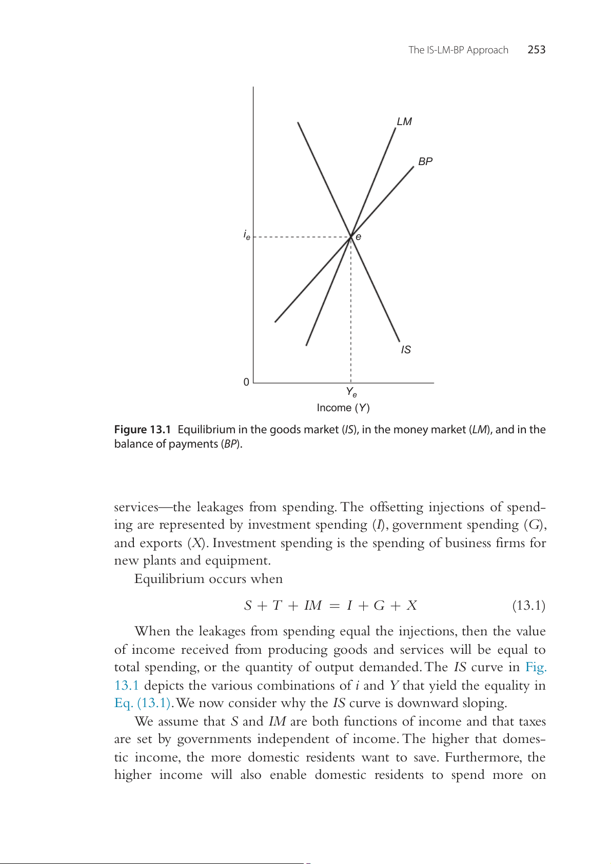
We will analyze the macroeconomic equilibrium with a graph that
summarizes equilibrium in each market. Fig. 13.1 displays the IS-LM-BP
diagram. This graph illustrates various combinations of the domestic inter-
est rate (i) and domestic national income (Y) that yield an equilibrium in
the three markets considered here. THE IS CURVE
First, let us examine the IS curve, which represents combinations of i and
Y that provide equilibrium in the goods market when everything else
(like the price level) is held constant. Y refers to the total output as well
as the total income in the economy. Equilibrium occurs when the out-
put of goods and services is equal to the quantity of goods and services
demanded. In principles of economics classes, macroeconomic equilibrium
is said to exist when the “leakages equal the injections” of spending in
the economy. More precisely, domestic saving (S), taxes (T), and imports
(IM) represent income received that is not spent on domestic goods and The IS-LM-BP Approach 253 LM BP )i (te ra ie st e re te In IS 0 Ye Income (Y )
Figure 13.1 Equilibrium in the goods market (IS), in the money market (LM), and in the balance of payments (BP).
services—the leakages from spending. The offsetting injections of spend-
ing are represented by investment spending (I), government spending (G),
and exports (X). Investment spending is the spending of business firms for new plants and equipment. Equilibrium occurs when
S + T + IM = I + G + X (13.1)
When the leakages from spending equal the injections, then the value
of income received from producing goods and services will be equal to
total spending, or the quantity of output demanded. The IS curve in Fig.
13.1 depicts the various combinations of i and
Y that yield the equality in
Eq. (13.1). We now consider why the IS curve is downward sloping.
We assume that S and IM are both functions of income and that taxes
are set by governments independent of income. The higher that domes-
tic income, the more domestic residents want to save. Furthermore, the
higher income will also enable domestic residents to spend more on 254
International Money and Finance i C C ) i A i A ( te ra st B iB re te In IS 0 ) X YC Y Y A B + ) G IM +I S + T + IM + ( T rts + o (S xp e rts o + p g in B I' + G + X im d + n e s A xe v. sp I + G + X ta o + g g C n t + I'' + G + X vi n a e S m st ve In 0 YC YA YB Income (Y)
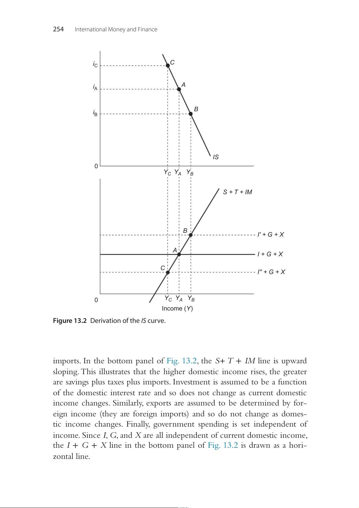
Figure 13.2 Derivation of the IS curve.
imports. In the bottom panel of Fig. 13.2, the S+ T + IM line is upward
sloping. This illustrates that the higher domestic income rises, the greater
are savings plus taxes plus imports. Investment is assumed to be a function
of the domestic interest rate and so does not change as current domestic
income changes. Similarly, exports are assumed to be determined by for-
eign income (they are foreign imports) and so do not change as domes-
tic income changes. Finally, government spending is set independent of
income. Since I, G, and X are all independent of current domestic income,
the I + G + X line in the bottom panel of Fig. 13.2 is drawn as a hori- zontal line. The IS-LM-BP Approach 255
Eq. (13.1) indicated that equilibrium occurs at that income level where
S + T + IM = I + G + X. In the bottom panel of Fig. 13.2, point A repre-
sents an equilibrium point with an equilibrium level of income YA. In the
upper panel of the figure, YA is shown to be consistent with point A on the
IS curve. This point is also associated with a particular interest rate iA.
To understand why the IS curve slopes downward, consider what hap-
pens as the interest rate varies. Suppose the interest rate falls. At the lower
interest rate, more potential investment projects become profitable (firms
will not require as high a return on investment when the cost of borrowed
funds falls), so investment increases as illustrated in the move from I + G +
X to I′ + G + X in Fig. 13.2. At this higher level of investment spending,
equilibrium income increases to YB. Point B on the IS curve depicts this
new goods market equilibrium, with a lower equilibrium interest rate iB
and higher equilibrium income YB.
Finally, consider what happens when the interest rate rises. Investment
spending will fall, because fewer potential projects are profitable as the cost
of borrowed funds rises. At the lower level of investment spending, the
I + G + X curve shifts down to I″ + G + X in Fig. 13.2. The new equi-
librium point C is consistent with the level of income YC. In the IS
diagram in the upper panel we see that point C is consistent with equi-
librium income level YC and equilibrium interest rate iC. The other points
on the IS curve are consistent with alternative combinations of income
and interest rate that yield equilibrium in the goods market.
We must remember that the IS curve is drawn holding the domestic
price level constant. A change in the domestic price level will change the
price of domestic goods relative to foreign goods. If the domestic price
level falls with a given interest rate, then investment, government spending,
taxes, and saving will not change. However, domestic goods are now cheaper
relative to foreign goods, leading to exports increasing and imports falling.
The rise in the I + G + X curve and the fall in the S + T + IM curve
would both increase income. Because income increases with a constant
interest rate, the IS curve shifts to the right. A rise in the domestic price
level would cause the IS curve to shift left. THE LM CURVE
The LM curve in Fig. 13.1 displays the alternative combinations of i and
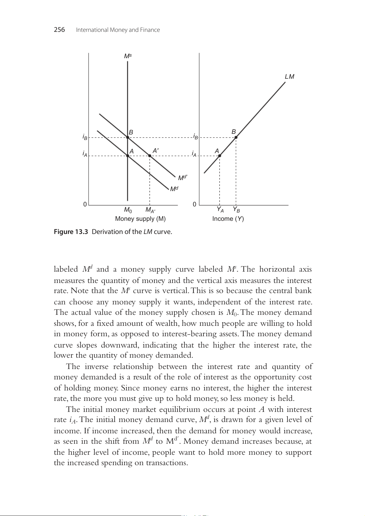
Y at which the demand for money equals the supply. Fig. 13.3 provides a
derivation of the LM curve. The left panel shows a money demand curve 256
International Money and Finance Ms LM )i ( te ra st B B re i i B B te In A A' i i A A A Md' Md 0 0 M Y Y 0 MA' A B Money supply (M) Income (Y)
Figure 13.3 Derivation of the LM curve.
labeled Md and a money supply curve labeled Ms. The horizontal axis
measures the quantity of money and the vertical axis measures the interest
rate. Note that the Ms curve is vertical. This is so because the central bank
can choose any money supply it wants, independent of the interest rate.
The actual value of the money supply chosen is M0. The money demand
shows, for a fixed amount of wealth, how much people are willing to hold
in money form, as opposed to interest-bearing assets. The money demand
curve slopes downward, indicating that the higher the interest rate, the
lower the quantity of money demanded.
The inverse relationship between the interest rate and quantity of
money demanded is a result of the role of interest as the opportunity cost
of holding money. Since money earns no interest, the higher the interest
rate, the more you must give up to hold money, so less money is held.
The initial money market equilibrium occurs at point A with interest
rate iA. The initial money demand curve, Md, is drawn for a given level of
income. If income increased, then the demand for money would increase,
as seen in the shift from Md to Md′. Money demand increases because, at
the higher level of income, people want to hold more money to support
the increased spending on transactions. The IS-LM-BP Approach 257
Now let us consider why the LM curve has a positive slope. Suppose ini-
tially there is equilibrium at point A with the interest rate at iA and income
at YA in Fig. 13.3. If income increases from YA to YB, money demand
increases from Md to Md′. If the interest rate remains at iA, there will be an
excess demand for money. This is shown in the left panel of Fig. 13.3, as the
quantity of money demanded is now MA′. With the higher income, money
demand is given by Md′. At iA, point A′ on the money demand curve is con-
sistent with the higher quantity of money demanded, MA′. Since the money
supply remains constant at M0, there will be an excess demand for money
given by MA′ − M0. The attempt to increase money balances above the
quantity of money outstanding will cause the interest rate to rise until a new
equilibrium is established at point B. This new equilibrium is consistent with
a higher interest rate iB and a higher income YB. Points A and B are both
indicated on the LM curve in the right panel of Fig. 13.3. The rest of the LM
curve reflects similar combinations of equilibrium interest rates and income.
The LM curve is drawn for a specific money supply. If the supply of
money increases, then money demand will have to increase to restore
equilibrium. This requires a higher
Y or lower i, or both, so the LM curve
will shift right. Similarly, a decrease in the money supply will tend to raise
i and lower Y, and the LM curve will shift to the left. THE BP CURVE
The final curve portrayed in Fig. 13.1 is the BP curve. The BP curve gives
the combinations of i and Y that yield balance of payments equilibrium.
The BP curve is drawn for a given domestic price level, a given exchange
rate, and a given net foreign debt. Equilibrium occurs when the cur-
rent account surplus is equal to the capital account deficit. Recall from
Chapter3, The Balance of Payments that if there is a current account defi-
cit, then it has to be financed by a capital account surplus.
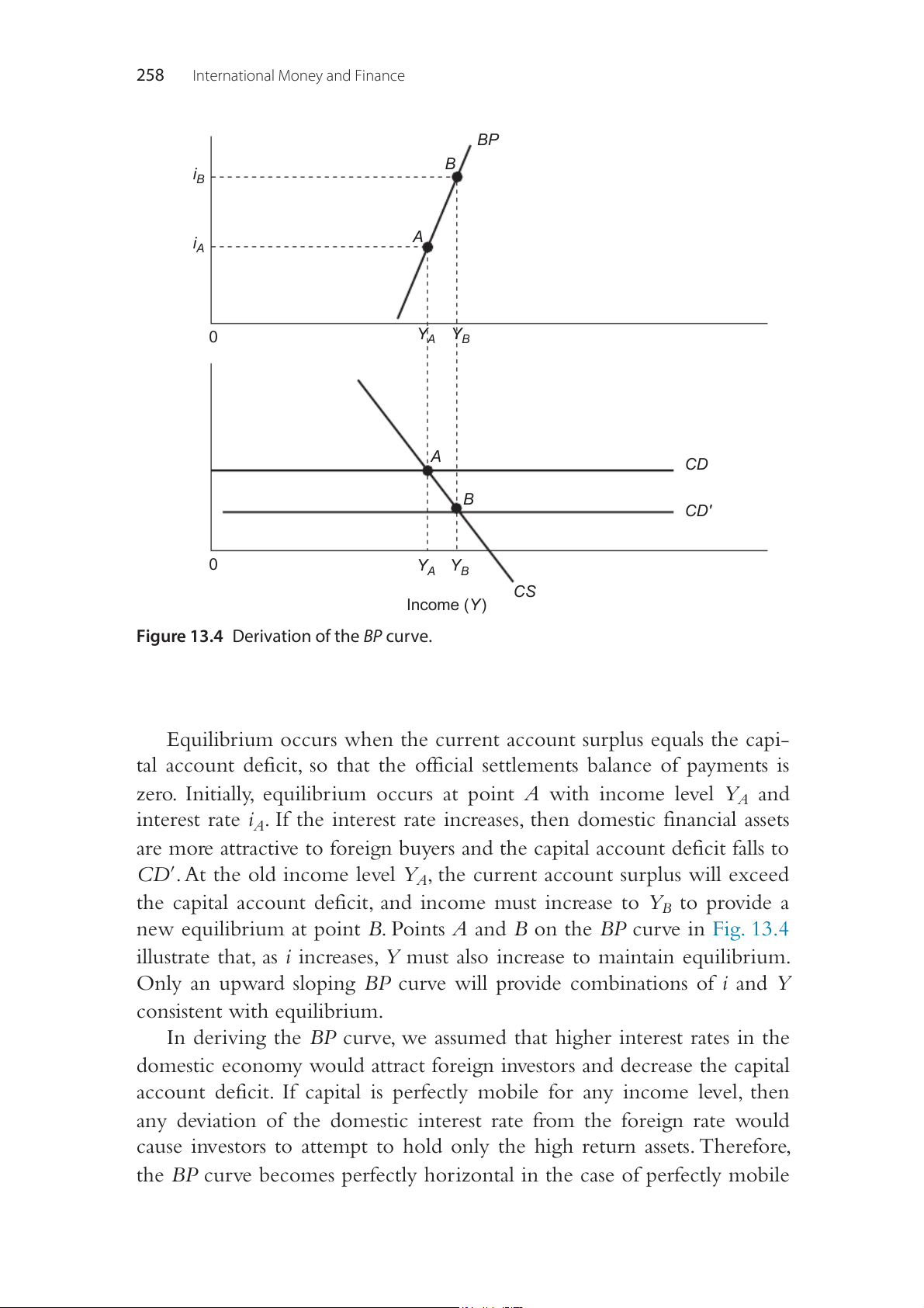
Fig. 13.4 illustrates the derivation of the BP curve. The lower panel
of the figure shows a CS line, representing the current account surplus,
and a CD line, representing the capital account deficit. Realistically, the
current account surplus may be negative, which would indicate a deficit.
Similarly, the capital account deficit may be negative, indicating a surplus.
The CS line is downward sloping because as income increases, domestic
imports increase and the current account surplus falls. The capital account
is assumed to be a function of the interest rate and is, therefore, indepen-
dent of income and a horizontal line. 258
International Money and Finance BP B iB )i (te A iA ra st re te In 0 YA YB S D C = C s t = lu rp fici e t su t d n n u A u CD cco cco l a B t a n CD' ita rre p u a C C 0 YA YB CS Income (Y )
Figure 13.4 Derivation of the BP curve.
Equilibrium occurs when the current account surplus equals the capi-
tal account deficit, so that the official settlements balance of payments is
zero. Initially, equilibrium occurs at point A with income level YA and
interest rate iA. If the interest rate increases, then domestic financial assets
are more attractive to foreign buyers and the capital account deficit falls to
CD′. At the old income level YA, the current account surplus will exceed
the capital account deficit, and income must increase to YB to provide a
new equilibrium at point B. Points A and B on the BP curve in Fig. 13.4
illustrate that, as i increases,
Y must also increase to maintain equilibrium.
Only an upward sloping BP curve will provide combinations of i and Y consistent with equilibrium.
In deriving the BP curve, we assumed that higher interest rates in the
domestic economy would attract foreign investors and decrease the capital
account deficit. If capital is perfectly mobile for any income level, then
any deviation of the domestic interest rate from the foreign rate would
cause investors to attempt to hold only the high return assets. Therefore,
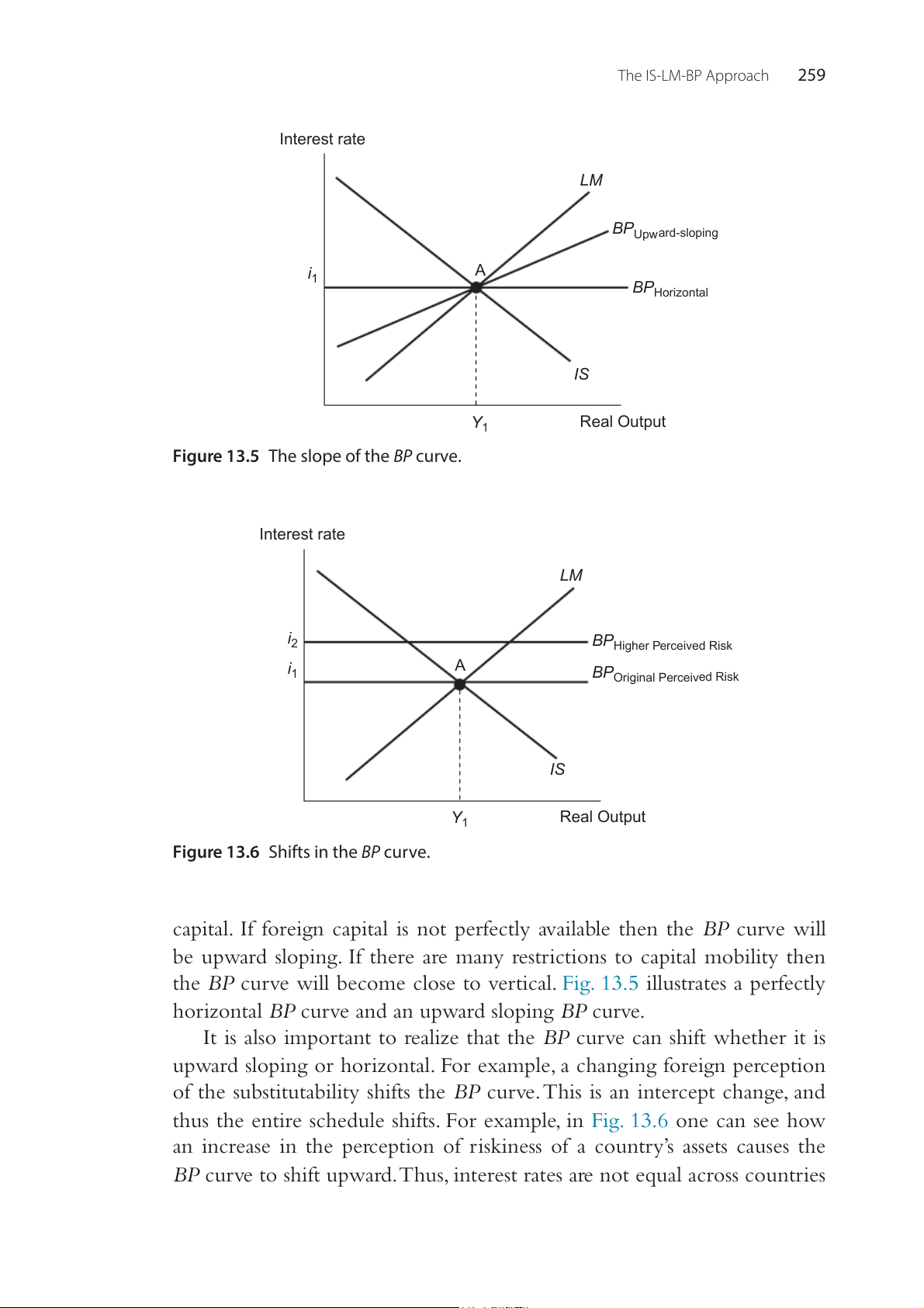
the BP curve becomes perfectly horizontal in the case of perfectly mobile The IS-LM-BP Approach 259 Interest rate LM BPUpward-sloping i A 1 BPHorizontal IS Y Real Output 1
Figure 13.5 The slope of the BP curve. Interest rate LM i2 BPHigher Perceived Risk i A 1
BPOriginal Perceived Risk IS Y Real Output 1
Figure 13.6 Shifts in the BP curve.
capital. If foreign capital is not perfectly available then the BP curve will
be upward sloping. If there are many restrictions to capital mobility then
the BP curve will become close to vertical. Fig. 13.5 illustrates a perfectly
horizontal BP curve and an upward sloping BP curve.
It is also important to realize that the BP curve can shift whether it is
upward sloping or horizontal. For example, a changing foreign perception
of the substitutability shifts the BP curve. This is an intercept change, and
thus the entire schedule shifts. For example, in Fig. 13.6 one can see how
an increase in the perception of riskiness of a country’s assets causes the
BP curve to shift upward. Thus, interest rates are not equal across countries 260
International Money and Finance
even with perfect capital mobility. For example, Indonesia may have a pos-
itive risk premium, so that investors demand a certain added premium for
financing Indonesia’s trade deficits. However, as long as that particular risk
premium is paid, investors are willing to finance the trade deficit. EQUILIBRIUM
Equilibrium for the economy requires that all three markets—the goods
market, the money market, and the balance of payments—be in equilib-
rium. This occurs when the IS, LM, and BP curves intersect at a common
equilibrium level of the interest rate and income. In Fig. 13.1, point e is
the equilibrium point that occurs at the equilibrium interest rate ie and
the equilibrium income level Ye. Until some change occurs that shifts one
of the curves, the IS-LM-BP equilibrium will be consistent with all goods
produced being sold, money demand equal to money supply, and a current
account surplus equal to a capital account deficit that yields a zero balance
on the official settlements account.
MONETARY POLICY UNDER FIXED EXCHANGE RATES
With fixed exchange rates, the domestic central bank is not free to con-
duct monetary policy independently from the rest of the world. If domes-
tic and foreign assets are perfect substitutes, then they must yield the same
return to investors. Clearly, in this case there is no room for central banks
to conduct an independent monetary policy under fixed exchange rates.
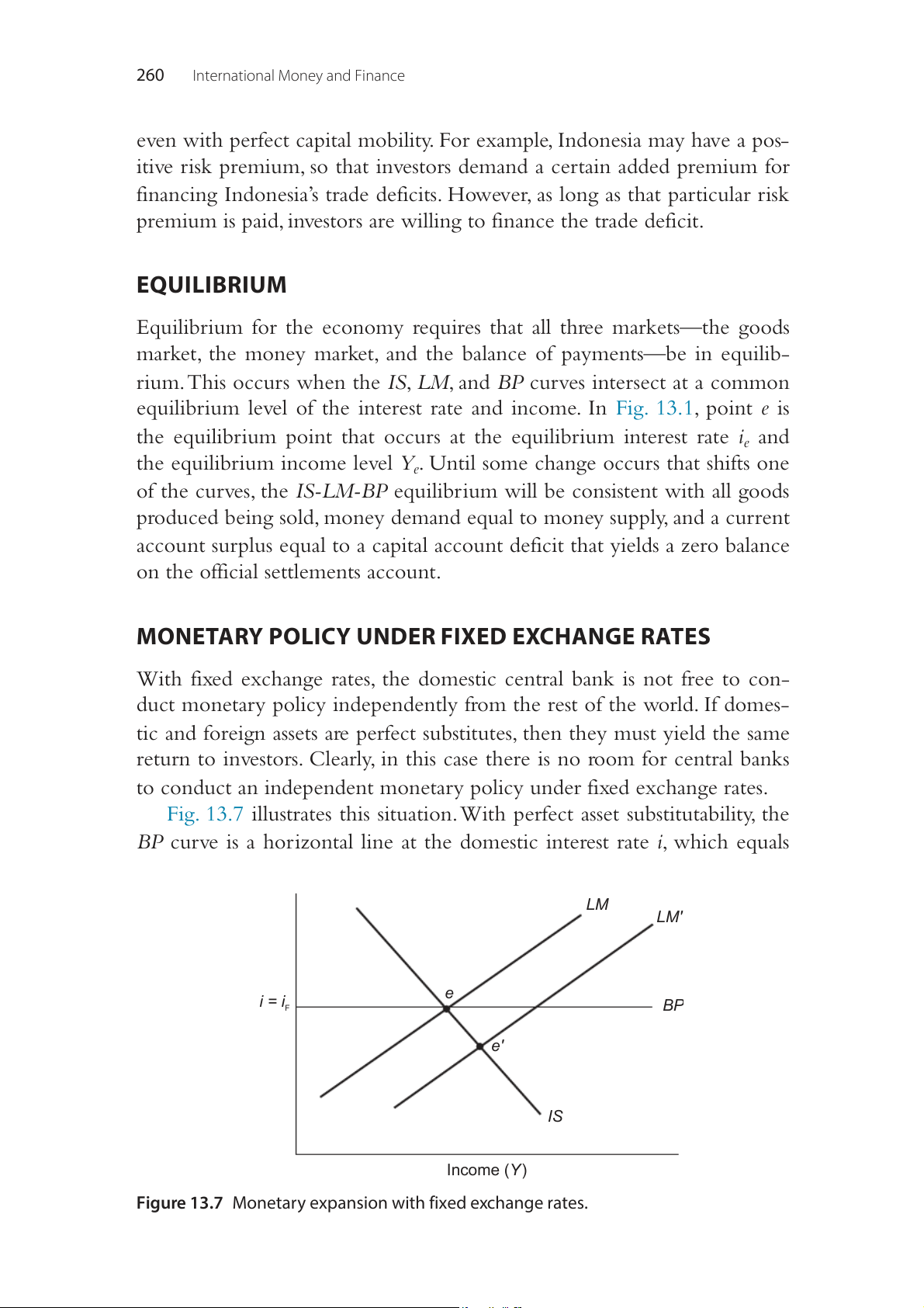
Fig. 13.7 illustrates this situation. With perfect asset substitutability, the
BP curve is a horizontal line at the domestic interest rate i, which equals LM LM' )i ( te e ra i = iF BP st re te e' In IS Income (Y )
Figure 13.7 Monetary expansion with fixed exchange rates. The IS-LM-BP Approach 261
the foreign interest rate iF. Any rate higher than iF results in large (infinite)
capital inflows, while any lower rate yields large capital outflows. Only at
iF is the balance of payments equilibrium obtained.
Suppose the central bank increases the money supply so that the LM
curve shifts from LM to LM′. The IS-LM equilibrium is now shifted from e
to e′. While e′ results in equilibrium in the money and goods market, there
will be a large capital outflow and large official settlements balance defi-
cit. This will pressure the domestic currency to depreciate on the foreign
exchange market. To maintain the fixed exchange rate, the central bank
must intervene and sell foreign exchange to buy domestic currency. The
foreign exchange market intervention will decrease the domestic money
supply and shift the LM curve back to LM to restore the initial equilibrium
at e. With perfect capital mobility, this would all happen instantaneously,
so that no movement away from point e is ever observed. Any attempt to
lower the money supply and shift the LM curve to the left would have just
the reverse effect on the interest rate and intervention activity.
If capital mobility is less than perfect, then the central bank has some
opportunity to vary the money supply. Still, the maintenance of the fixed
exchange rate will require an ultimate reversal of policy in the face of a
constant foreign interest rate. The process is essentially just drawn out over
time rather than occurring instantly.
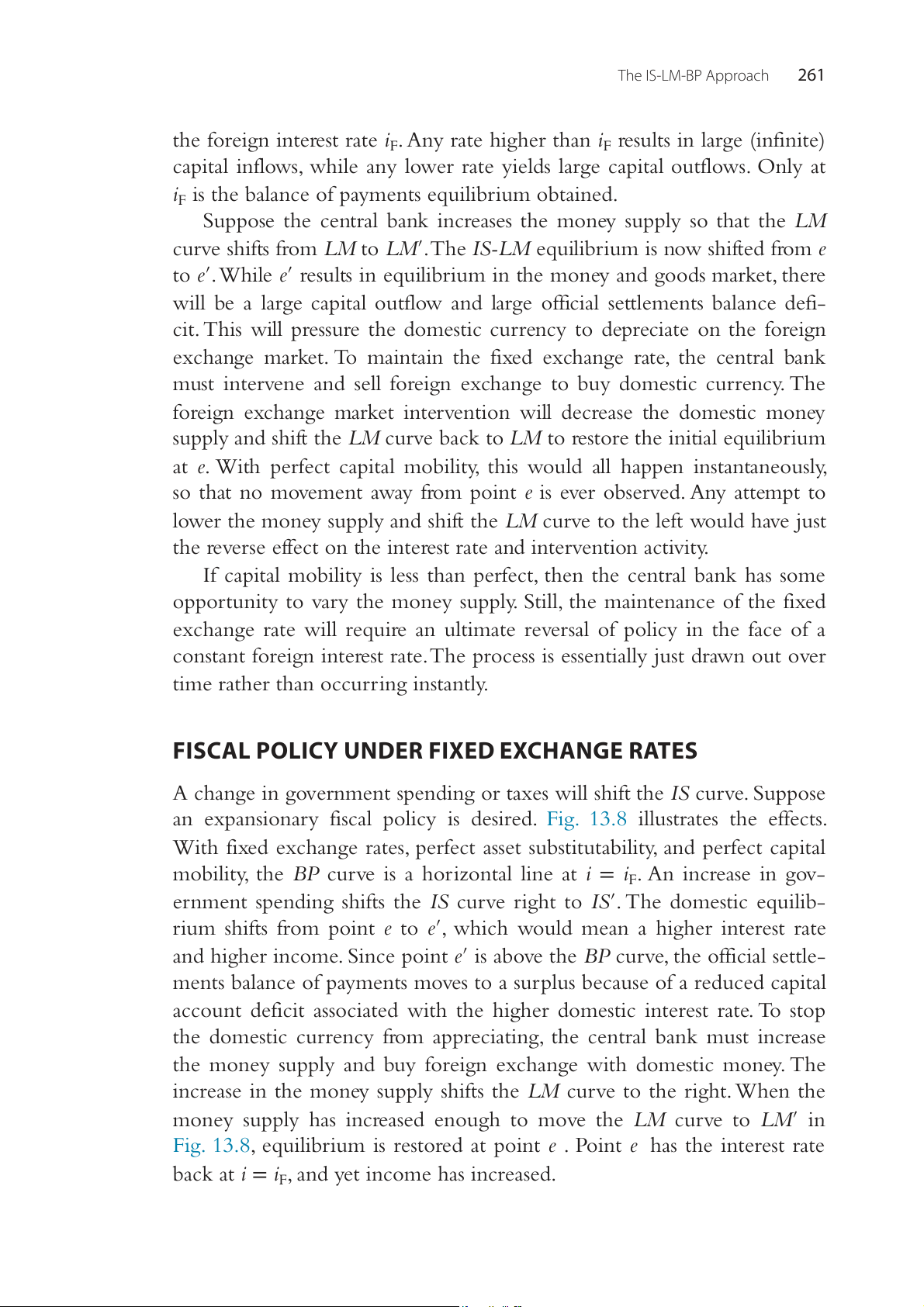
FISCAL POLICY UNDER FIXED EXCHANGE RATES
A change in government spending or taxes will shift the IS curve. Suppose
an expansionary fiscal policy is desired. Fig. 13.8 illustrates the effects.
With fixed exchange rates, perfect asset substitutability, and perfect capital
mobility, the BP curve is a horizontal line at i = iF. An increase in gov-
ernment spending shifts the IS curve right to IS′. The domestic equilib-
rium shifts from point e to e′, which would mean a higher interest rate
and higher income. Since point e′ is above the BP curve, the official settle-
ments balance of payments moves to a surplus because of a reduced capital
account deficit associated with the higher domestic interest rate. To stop
the domestic currency from appreciating, the central bank must increase
the money supply and buy foreign exchange with domestic money. The
increase in the money supply shifts the LM curve to the right. When the
money supply has increased enough to move the LM curve to LM′ in
Fig. 13.8, equilibrium is restored at point e". Point e" has the interest rate
back at i = iF, and yet income has increased. 262
International Money and Finance LM LM' )i e' ( te e e'' ra i = iF BP st re te In IS' IS Income (Y )
Figure 13.8 Fiscal expansion with fixed exchange rates.
This result is a significant difference from the monetary policy expan-
sion considered in the preceding section. With fixed exchange rates and
perfect capital mobility, monetary policy was seen to be ineffective in
changing the level of income. This was so because there was no room for
independent monetary policy with a fixed exchange rate. In contrast, fis-
cal policy will have an effect on income and can be used to stimulate the domestic economy.
MONETARY POLICY UNDER FLOATING EXCHANGE RATES
We now consider a world of flexible exchange rates and perfect capital
mobility. The notable difference between the analysis in this section and
the fixed exchange rate stories of the previous two sections is that with
floating rates the central bank is not obliged to intervene in the foreign
exchange market to support a particular exchange rate. With no interven-
tion, the current account surplus will equal the capital account deficit so
that the official settlements balance equals zero. In addition, since the cen-
tral bank does not intervene to fix the exchange rate, the money supply can
change to any level desired by the monetary authorities. This independence
of monetary policy is one of the advantages of flexible exchange rates.
The assumptions of perfect substitutability of assets and perfect capital
mobility will result in i = iF as before. Once again, the BP curve will be a
horizontal line at i = iF. Only now, equilibrium in the balance of payments
will mean a zero official settlements balance. Changes in the exchange rate
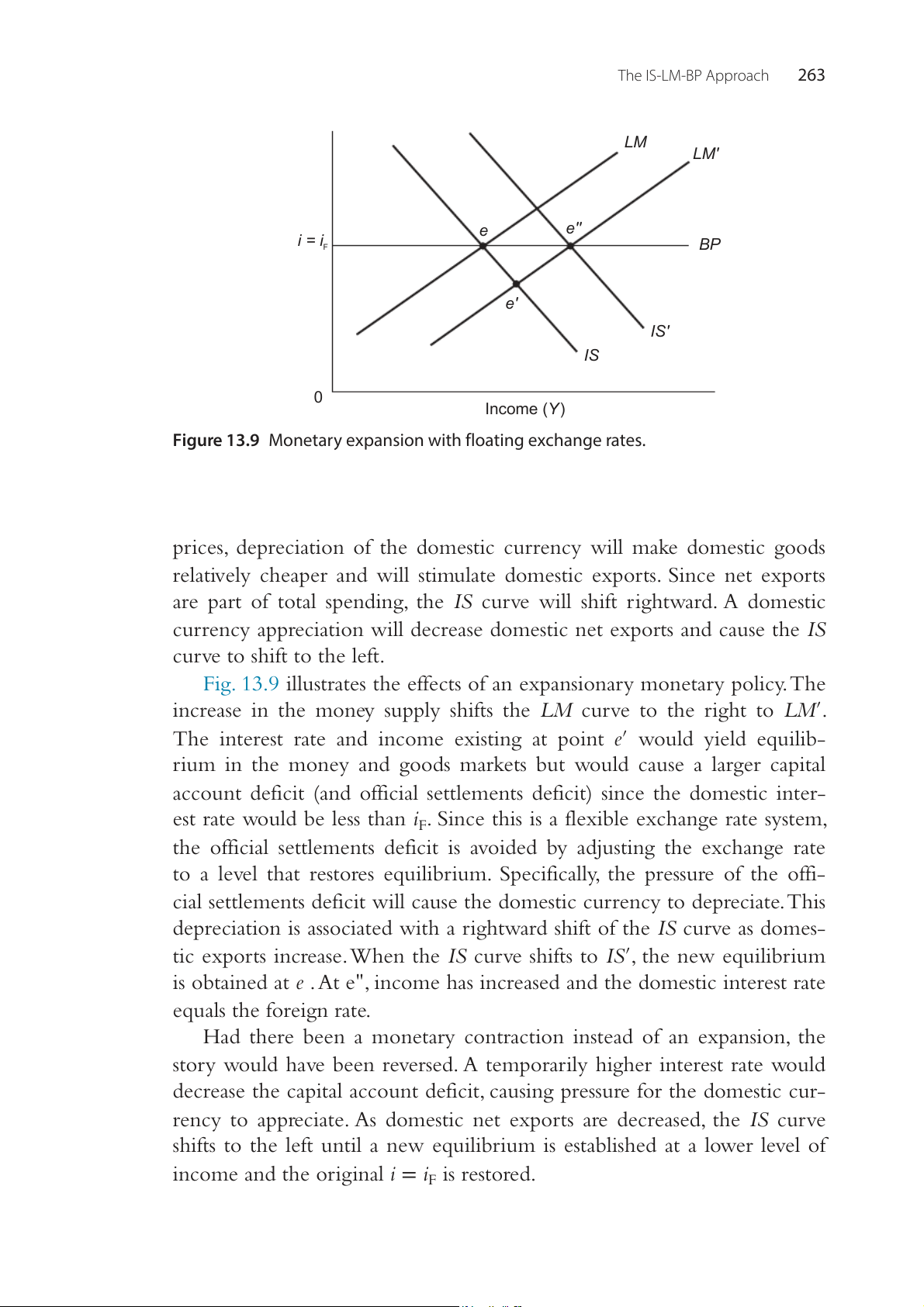
will cause shifts in the IS curve. With fixed domestic and foreign goods The IS-LM-BP Approach 263 LM LM' )i ( te e e'' ra i = iF BP st re te In e' IS' IS 0 Income (Y )
Figure 13.9 Monetary expansion with floating exchange rates.
prices, depreciation of the domestic currency will make domestic goods
relatively cheaper and will stimulate domestic exports. Since net exports
are part of total spending, the IS curve will shift rightward. A domestic
currency appreciation will decrease domestic net exports and cause the IS curve to shift to the left.
Fig. 13.9 illustrates the effects of an expansionary monetary policy. The
increase in the money supply shifts the LM curve to the right to LM′.
The interest rate and income existing at point e′ would yield equilib-
rium in the money and goods markets but would cause a larger capital
account deficit (and official settlements deficit) since the domestic inter-
est rate would be less than iF. Since this is a flexible exchange rate system,
the official settlements deficit is avoided by adjusting the exchange rate
to a level that restores equilibrium. Specifically, the pressure of the offi-
cial settlements deficit will cause the domestic currency to depreciate. This
depreciation is associated with a rightward shift of the IS curve as domes-
tic exports increase. When the IS curve shifts to IS′, the new equilibrium
is obtained at e". At e", income has increased and the domestic interest rate equals the foreign rate.
Had there been a monetary contraction instead of an expansion, the
story would have been reversed. A temporarily higher interest rate would
decrease the capital account deficit, causing pressure for the domestic cur-
rency to appreciate. As domestic net exports are decreased, the IS curve
shifts to the left until a new equilibrium is established at a lower level of
income and the original i = iF is restored. 264
International Money and Finance
In contrast to the fixed exchange rate world, monetary policy can
change the level of income with floating exchange rates. Since the exchange
rate adjusts to yield balance of payments equilibrium, the central bank
can choose its monetary policy independent of other countries’ policies.
This world of flexible exchange rates and perfect capital mobility is often
called the Mundell–Fleming model of the open economy. (Robert Mundell,
Nobel Laureate in Economics in 1999, and Marcus Fleming were two early
researchers who developed models along the lines of those presented here.)
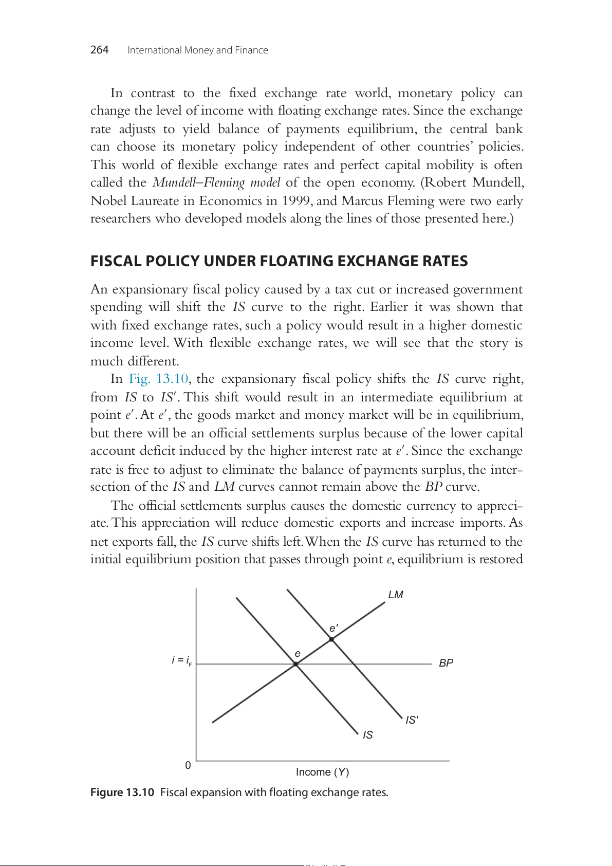
FISCAL POLICY UNDER FLOATING EXCHANGE RATES
An expansionary fiscal policy caused by a tax cut or increased government
spending will shift the IS curve to the right. Earlier it was shown that
with fixed exchange rates, such a policy would result in a higher domestic
income level. With flexible exchange rates, we will see that the story is much different.
In Fig. 13.10, the expansionary fiscal policy shifts the IS curve right,
from IS to IS′. This shift would result in an intermediate equilibrium at
point e′. At e′, the goods market and money market will be in equilibrium,
but there will be an official settlements surplus because of the lower capital
account deficit induced by the higher interest rate at e′. Since the exchange
rate is free to adjust to eliminate the balance of payments surplus, the inter-
section of the IS and LM curves cannot remain above the BP curve.
The official settlements surplus causes the domestic currency to appreci-
ate. This appreciation will reduce domestic exports and increase imports. As
net exports fall, the IS curve shifts left. When the IS curve has returned to the
initial equilibrium position that passes through point e, equilibrium is restored LM )i e' ( te e ra i = iF BP st re te In IS' IS 0 Income (Y )
Figure 13.10 Fiscal expansion with floating exchange rates. The IS-LM-BP Approach 265
in all markets. Note that the final equilibrium occurs at the initial level of i
and Y. With floating exchange rates, fiscal policy is ineffective in shifting the
level of income. When an expansionary fiscal policy has no effect on income,
complete crowding out has occurred. Crowding out means that the positive
effect on income is offset by a reduction of income from another factor. For
example, when the economy moves from e to e′ the investment spending
will be reduced. This will partially crowd out the positive effect of the expan-
sionary fiscal policy. However, when the domestic currency appreciates and
the economy returns to e, then the crowding out effect occurs because the
currency appreciation induced by the expansionary fiscal policy reduces net
exports to a level that just offsets the fiscal policy effects on income.
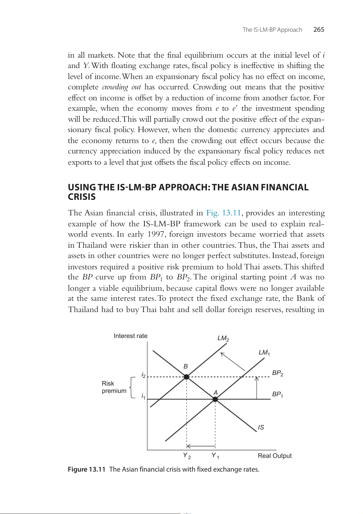
USING THE IS-LM-BP APPROACH: THE ASIAN FINANCIAL CRISIS
The Asian financial crisis, illustrated in Fig. 13.11, provides an interesting
example of how the IS-LM-BP framework can be used to explain real-
world events. In early 1997, foreign investors became worried that assets
in Thailand were riskier than in other countries. Thus, the Thai assets and
assets in other countries were no longer perfect substitutes. Instead, foreign
investors required a positive risk premium to hold Thai assets. This shifted
the BP curve up from BP1 to BP2. The original starting point A was no
longer a viable equilibrium, because capital flows were no longer available
at the same interest rates. To protect the fixed exchange rate, the Bank of
Thailand had to buy Thai baht and sell dollar foreign reserves, resulting in Interest rate LM2 LM1 B BP i 2 2 Risk premium A BP i 1 1 IS Y Y Real Output 2 1
Figure 13.11 The Asian financial crisis with fixed exchange rates. 266
International Money and Finance
a reduction in money supply in Thailand. This shifted the LM curve from
LM1 to LM2. This monetary tightening also caused the domestic inter-
est rates to sharply increase, crowding out domestic private investment.
Thailand went into a deep recession.
Speculators sensed that the Bank of Thailand could not keep on pro-
tecting the Thai baht. Therefore they sold their assets denominated in Thai
baht and bought dollar assets. This led to further pressure on the Thai baht
to depreciate. After a considerable effort in trying to protect the fixed
exchange rate, the Thai government and Bank of Thailand decided to
allow the exchange rate to float on July 2, 1997. The Thai baht immedi-
ately depreciated from 25 baht per dollar to over 50 baht per dollar. With
a floating rate the response to the risk premium demanded by the spec-
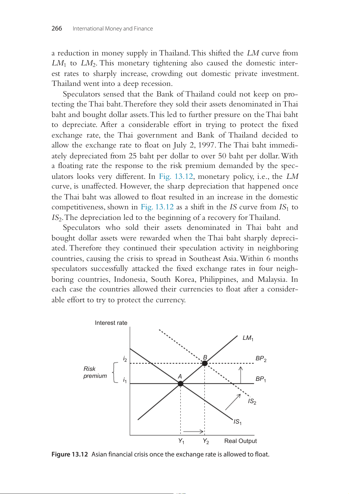
ulators looks very different. In Fig. 13.12, monetary policy, i.e., the LM
curve, is unaffected. However, the sharp depreciation that happened once
the Thai baht was allowed to float resulted in an increase in the domestic
competitiveness, shown in Fig. 13.12 as a shift in the IS curve from IS1 to
IS2. The depreciation led to the beginning of a recovery for Thailand.
Speculators who sold their assets denominated in Thai baht and
bought dollar assets were rewarded when the Thai baht sharply depreci-
ated. Therefore they continued their speculation activity in neighboring
countries, causing the crisis to spread in Southeast Asia. Within 6 months
speculators successfully attacked the fixed exchange rates in four neigh-
boring countries, Indonesia, South Korea, Philippines, and Malaysia. In
each case the countries allowed their currencies to float after a consider-
able effort to try to protect the currency. Interest rate LM1 i B BP 2 2 Risk premium A i BP 1 1 IS2 IS1 Y1 Y2 Real Output
Figure 13.12 Asian financial crisis once the exchange rate is allowed to float. The IS-LM-BP Approach 267
FAQ: How Did the Asian Financial Crisis Start?
In early 1997, hedge funds believed that the Thai baht was pegged at a too high
value and took positions against the baht. The central bank of Thailand did not
allow the Thai baht to float, but instead heavily supported it, spending about
US$30 billion in a 6-month period. The response by the central bank caused
losses to the speculators, but made them even more determined to bet against
the Thai baht. The hedge funds knew that the central bank could not maintain
its defense over a longer period, and renewed their bets. On one single day
alone, on May 14, 1997, speculators had bet US$10 billion against the baht. To
compound the problems for Thailand, Japanese banks decided to move assets
out of Thailand. The Japanese banks were some of the biggest investors in
Thailand, but were already hurt by domestic debt defaults. Therefore, they were
quick to withdraw their assets from Thailand.
Pressure from speculators, combined with internal political pressure, finally
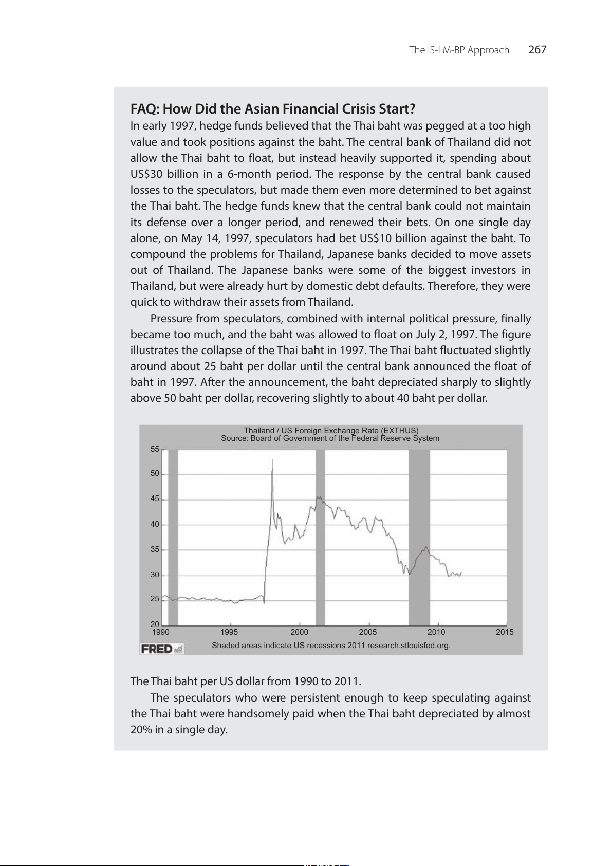
became too much, and the baht was allowed to float on July 2, 1997. The figure
illustrates the collapse of the Thai baht in 1997. The Thai baht fluctuated slightly
around about 25 baht per dollar until the central bank announced the float of
baht in 1997. After the announcement, the baht depreciated sharply to slightly
above 50 baht per dollar, recovering slightly to about 40 baht per dollar.
Thailand / US Foreign Exchange Rate (EXTHUS)
Source: Board of Government of the Federal Reserve System 55 50 ) llar 45 o D S U 40 e n O 35 t to h a i B a 30 h (T 25 20 1990 1995 2000 2005 2010 2015
Shaded areas indicate US recessions 2011 research.stlouisfed.org.
The Thai baht per US dollar from 1990 to 2011.
The speculators who were persistent enough to keep speculating against
the Thai baht were handsomely paid when the Thai baht depreciated by almost 20% in a single day. 268
International Money and Finance
So why not allow the Thai baht to float earlier? A fixed exchange rate
encourages banks and firms not to cover the exchange rate exposure. Thus,
banks had short-term loans in dollars and long-term investments in Thai
baht. A devaluation of the Thai baht would create difficulty for banks in
Thailand, as the cost of paying their debt would exceed the return on their
long-term investments. This is typical for many developing countries in
that the government encourages local investment and borrows from capital
rich developed countries. Thus, banks in Thailand had a large number of
loans in dollars and payments in baht. After the depreciation of the dollar,
most of the banks and financial firms went bankrupt, with over 50 banks
and financial firms taken over by the Thai government in the end of 1997.
INTERNATIONAL POLICY COORDINATION
From the early 1970s onward, the major developed nations have generally
operated with floating exchange rates. The IS-LM-BP framework, ana-
lyzed in this chapter, has shown that fiscal and monetary policy can gener-
ate large swings in floating exchange rates. Economists have been debating
how to coordinate policies across countries, because of the potential dis-
ruptive effect of exchange rate volatility on world trade.
The high degree of capital mobility existing among the developed
countries suggests that fiscal actions that lead to a divergence of the
domestic interest rate from the given foreign interest rate will quickly
be undone by the influence of exchange rate changes on net exports, as
was illustrated in Fig. 13.10. For example, many economists argue that
the sharp increase in the dollar value in the early 1980s was due to the
expansionary fiscal policy followed by the US government. How could
such exchange rate volatility be minimized? If all nations coordinated
their domestic policies and simultaneously stimulated their economies,
the world interest rate would rise. Thus, the pressure for an exchange
rate change for a particular country (in the above case, the United States)
would disappear. The problem illustrated in Fig. 13.10 was that of a sin-
gle country attempting to follow an expansionary policy while the rest
of the world retained unchanged policies, so that iF remains constant. If
iF increased at the same time that i increased, the BP curve would shift
upward and the balance of payments equilibrium would be consistent with a higher interest rate.
Similarly, changes in exchange rates and net exports induced by mon-
etary policy can be lessened if central banks coordinate policy so that iF The IS-LM-BP Approach 269
shifts with i. There have been instances of coordinated foreign exchange
market intervention when a group of central banks jointly followed poli-
cies aimed at a depreciation or appreciation of the dollar. These coordi-
nated interventions, intended to achieve a target value of the dollar, also
work to bring domestic monetary policies more in line with each other.
If the United States has been following an expansionary monetary policy
relative to Japan, US interest rates may fall relative to the other country’s
rates, so that a larger capital account deficit is induced and pressure for a
dollar depreciation results. If the central banks decide to work together
to stop the dollar depreciation, the Japanese will buy dollars on the for-
eign exchange market with their domestic currencies, while the Federal
Reserve must sell foreign exchange to buy dollars. This will result in a
higher money supply in Japan and a lower money supply in the United
States. The coordinated intervention works toward a convergence of mon- etary policy in each country.
The basic argument in favor of international policy coordination is
that such coordination would stabilize exchange rates. Whether exchange
rate stability offers any substantial benefits over freely floating rates with
independent policies is a matter of much debate. Some experts argue that
coordinated monetary policy to achieve fixed exchange rates or to reduce
exchange rate fluctuations to within narrow target zones would reduce
the destabilizing aspects of international trade in goods and financial assets
when currencies become overvalued or undervalued. This view empha-
sizes that in an increasingly integrated world economy, it seems desirable
to conduct national economic policy in an international context rather
than by simply focusing on domestic policy goals without a view of the international implications.
An alternative view is that most changes in exchange rates result from
real economic shocks and should be considered permanent changes. In
this view, there is no such thing as an overvalued or undervalued currency
because exchange rates always are in equilibrium given current economic
conditions. Furthermore, governments cannot change the real relative prices
of goods internationally by driving the nominal exchange rate to some par-
ticular level through foreign exchange market intervention, because price
levels will adjust to the new nominal exchange rate. This view, then, argues
that government policy is best aimed at lowering inflation and achieving
governmental goals that contribute to a stable domestic economy.
The debate over the appropriate level and form of international pol-
icy coordination has been one of the livelier areas of international finance 270
International Money and Finance
in recent years. Many leading economists have participated, but a prob-
lem at the practical level is that different governments emphasize different
goals and may view the current economic situation differently. Ours is a
more complex world in which to formulate international policy agree-
ments than is typically viewed in scholarly debate, where it is presumed
that governments agree on the current problems and on the impact of
alternative policies on those problems. Nevertheless, the research of inter-
national financial scholars offers much promise in contributing toward a
greater understanding of the real-world complexities government officials must address. SUMMARY
1. The desired economic outcome in an open economy is to achieve
both internal balance and external balance at the same time.
2. Internal balance refers to a domestic equilibrium condition such that
goods market and money market are in equilibrium and unemploy- ment is at its natural level.
3. External balance requires the balance of payments to be in equilib-
rium. The condition implies zero balance on the official settlement—
the current account surplus must be equal to the capital account deficit.
4. The IS curve represents the combinations of income and interest rate
levels that bring the good market to equilibrium (i.e., leakages equals to injections).
5. The LM curve represents the combinations of income and interest
rate levels that bring the money market to equilibrium (i.e., money
demand equals to money supply).
6. The BP curve represents the combinations of income and inter-
est rate levels that bring the balance of payments to equilibrium (i.e.,
current account surplus equals to capital account deficit).
7. The internal and external equilibriums occur when three curves intersect at one point.
8. The factors that shift the IS curve are a change in domestic price
level, a change in exchange rate, and a change in fiscal policy variable.
9. The factor that shifts the LM curve is a change in money supply.
10. The slope of the BP curve depends on the degree of capital mobil-
ity. In the case of perfect capital mobility between countries, the BP curve is horizontal.
Tài liệu liên quan:
-

Hoạt động Tài chính của Doanh nghiệp Đa Quốc Gia (DN) - Chương 6 | Tài chính quốc tế | Trường Học Viện nông nghiệp Việt Nam
19 10 -

Hệ Thống Tiền Tệ Quốc Tế: Khái Niệm và Các Chế Độ Tỷ Giá | Tài chính quốc tế | Trường Học Viện nông nghiệp Việt Nam
24 12 -

Bài giảng Chương 1: Các Quan Hệ Cân Bằng Quốc Tế và LOP | Tài chính quốc tế | Trường Học Viện nông nghiệp Việt Nam
21 11 -

Cách Tính Lạm Phát và CPI: So Sánh Việt Nam và Mỹ | Tài chính quốc tế | Trường Học Viện nông nghiệp Việt Nam
23 12 -

Detailed Report and Analysis on Submission Trends | Tài chính quốc tế | Trường Học Viện nông nghiệp Việt Nam
23 12