
Assignment 1 - Business Computing Skills | Trường Đại học Quốc tế, Đại học Quốc gia Thành phố HCM

Assignment 1 - Business Computing Skills | Trường Đại học Quốc tế, Đại học Quốc gia Thành phố HCM được sưu tầm và soạn thảo dưới dạng file PDF để gửi tới các bạn sinh viên cùng tham khảo, ôn tập đầy đủ kiến thức, chuẩn bị cho các buổi học thật tốt. Mời bạn đọc đón xem!

Thông tin:
3 trang 7 tháng trước

Bình luận

Vui lòng đăng nhập hoặc đăng ký để gửi bình luận.

Assignment 1 - Business Computing Skills | Trường Đại học Quốc tế, Đại học Quốc gia Thành phố HCM

Assignment 1 - Business Computing Skills | Trường Đại học Quốc tế, Đại học Quốc gia Thành phố HCM được sưu tầm và soạn thảo dưới dạng file PDF để gửi tới các bạn sinh viên cùng tham khảo, ôn tập đầy đủ kiến thức, chuẩn bị cho các buổi học thật tốt. Mời bạn đọc đón xem!

43 22 lượt tải Tải xuống
Assignment 1
Q1. Create a worksheet named In this worksheet, create the following Table. Summary.
Then, do as
follows:
a. Create
additional
column with
header
called
Revenue
Analysis.
Fill the
value in this
column as follows:
- Revenue
15000: take the corresponding value of Revenue
-
15,000<¿
Revenue
¿ 20,000
: Good
- Revenue
20,000: Exceptional
b. Create additional column with header called . Fill in this column by theThreshold Value
following equation
Threshold Value
=
Revenue
Budget
1
where
Threshold Value
is shown in the format of percentage (%)
c. Use conditional formatting to highlight any threshold value (%) which is negative value.
Also use the same method to highlight any information related to Whsapp (including
Revenue Budget, , ) Revenue analysis
d. Create additional table as follows
Largest threshold Smallest budget
Number of Good in
Revenue Analysis
No of both “good” in Revenue
Analysis which has budget less
than 15000
Order Application Name (Apps) Revenue Budget
01 GG $ 11,649 $ 10,593
02 Fa $ 7,718 $ 6,400
03 Blend $ 15,033 $ 12,700
04 Accord $ 18,701 $ 19,100
05 Misty Wash $ 14,432 $ 15,100
06 Whsapp $ 17,990 $ 18,008
07 Zal $ 11,022 $ 13,112
08 Mess $ 17,760 $ 16,854
09 Vivo $ 30,400 $ 30,327
10 Ymi $ 20,400 $ 18,444
Known that, in this table, Largest threshold and Smallest budget are filled up by using
VLOOKUP. COUNTIF and COUNTIFS can be used to calculate the values of remaining
columns.
e. Use the line chart with full format to display , , and Revenue Budget Threshold Value.
Q2.
Create the following table in a worksheet named as Book price
Month January February March April May June
Average Salary of
Employees
$ 1,500 $ 1,500 $ 1,600 $ 1,800 $ 1,900 $ 2,100
Books sold $ 2,000 $ 1,600 $ 4,000 $ 3,000 $ 2,300 $ 5,000
Table 3
a) Create another row called which is calculated byProfit
Profit=Books sold- Average Salary of Employees
Perform the calculation of for each month, January to June.Profit
b) Create a standard chart that can show the comparison of 3 data sets Average Salary of
Employees Profit, , and Books sold .
c) Create a Pivot Table in another spreadsheet named based on data given in Table as followsSum
Sum of
January
Sum of
February
Sum of
March
Sum of
April
Sum of May
Sum of
June
Average
Salary of
Employee
$ 1,500
$
1,500
$ 1,600 $ 1,800 $ 1,900 $ 2,100
Books sold $ 2,000
$
1,600
$ 4,000 $ 3,000 $ 2,300 $ 5,000
Grand Total $ 3,500
$
3,100
$ 5,600 $ 4,800 $ 4,200 $ 7,100
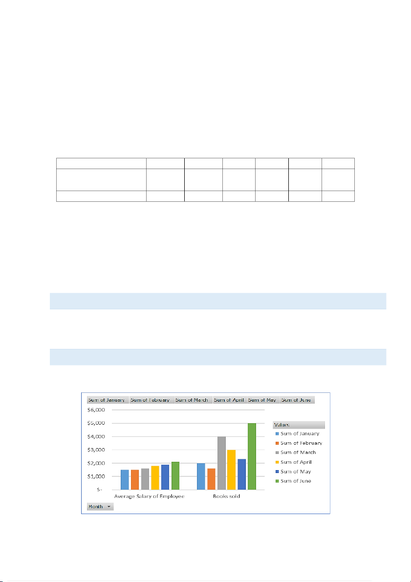
and then in the same spreadsheet, create a Pivot Chart based on the obtained Pivot Table as follows
d) Use appropriate chart to obtain the exact linear equation describing the future estimates of Profit
in the later 6 months, from July to December. Show clearly on the chart the obtained equation.
| 1/3

Preview text:

Assignment 1
Q1. Create a worksheet named Summary. In this worksheet, create the following Table. Order Application Name (Apps) Revenue Budget 01 GG $ 11,649 $ 10,593 Then, do as 02 Fa $ 7,718 $ 6,400 follows: 03 Blend $ 15,033 $ 12,700 a. Create 04 Accord $ 18,701 $ 19,100 additional 05 Misty Wash $ 14,432 $ 15,100 column with 06 Whsapp $ 17,990 $ 18,008 header called 07 Zal $ 11,022 $ 13,112 Revenue 08 Mess $ 17,760 $ 16,854 Analysis. 09 Vivo $ 30,400 $ 30,327 Fill the 10 Ymi $ 20,400 $ 18,444 value in this column as follows: -
Revenue 15000: take the corresponding value of Revenue -
15,000<¿ Revenue¿ 20,000: Good -
Revenue 20,000: Exceptional
b. Create additional column with header called Threshold Value. Fill in this column by the following equation Revenue Threshold Value= −1 Budget
where Threshold Value is shown in the format of percentage (%)
c. Use conditional formatting to highlight any threshold value (%) which is negative value.
Also use the same method to highlight any information related to Whsapp (including Revenue Budget , , Revenue analysis)
d. Create additional table as follows
No of both “good” in Revenue Number of Good in Largest threshold Smallest budget Analysis which has budget less Revenue Analysis than 15000
Known that, in this table, Largest threshold and Smallest budget are filled up by using
VLOOKUP. COUNTIF and COUNTIFS can be used to calculate the values of remaining columns.
e. Use the line chart with full format to display Revenue, Budget, and Threshold Value. Q2.
Create the following table in a worksheet named as Book price Month January February March April May June Average Salary of $ 1,500
$ 1,500 $ 1,600 $ 1,800 $ 1,900 $ 2,100 Employees Books sold $ 2,000
$ 1,600 $ 4,000 $ 3,000 $ 2,300 $ 5,000 Table 3
a) Create another row called Profit which is calculated by
Profit=Books sold- Average Salary of Employees
Perform the calculation of Profit for each month, January to June.
b) Create a standard chart that can show the comparison of 3 data sets Average Salary of
Employees, Books sold, and Profit.
c) Create a Pivot Table in another spreadsheet named Sum based on data given in Table as follows Sum of Sum of Sum of Sum of Sum of Sum of May January February March April June Average $ Salary of $ 1,500 $ 1,600 $ 1,800 $ 1,900 $ 2,100 1,500 Employee $ Books sold $ 2,000 $ 4,000 $ 3,000 $ 2,300 $ 5,000 1,600 $ Grand Total $ 3,500 $ 5,600 $ 4,800 $ 4,200 $ 7,100 3,100
and then in the same spreadsheet, create a Pivot Chart based on the obtained Pivot Table as follows
d) Use appropriate chart to obtain the exact linear equation describing the future estimates of Profit
in the later 6 months, from July to December. Show clearly on the chart the obtained equation.