Bài thuyết trình thống kê ứng dụng

Statistic for economics and finance Instructor: Pham Ha Forecasting with Time Series Analysis Chapter 5 5-1 Learning Objectives
LO5-1 Identify and describe time series patterns.
LO5-2 Compute forecasting using simple moving averages.
LO5-3 Compute and interpret the Mean Absolute Deviation.
LO5-4 Compute forecasts using exponential smoothing.
LO5-5 Compute a forecasting model using regression analysis.
LO5-6 Apply the Durban-Watson statistic to test for autocorrelation.
LO5-7 Compute seasonal indexes and use the indexes to
make seasonally adjusted forecasts. 5-2 Components of a Time Series
 A time series is a collection of data over a period of time
 The trend is the long-run direction of the time series
TREND PATTERN The change of a variable over time.
 The seasonal variation is a pattern that tends to repeat
itself from year to year for most businesses
SEASONALITY Patterns of highs and lows in a time series within a
calendar year. These patterns tend to repeat each year. 5-3
Components of a Time Series Continued
 The cyclical component is the fluctuation above and
below the long-term trend line over a longer time period
CYCLES A pattern of highs and lows occurring over periods of many years.
 The irregular variation is divided into episodic and residual components
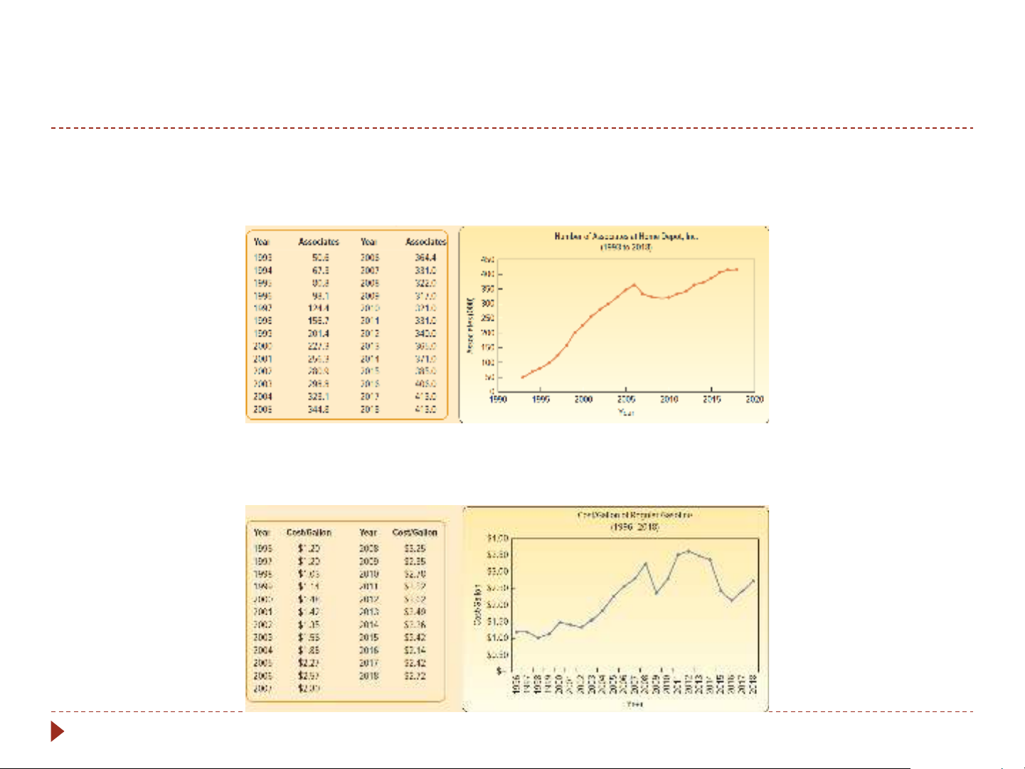
IRREGULAR COMPONENT The random variation in a time series. 5-4 Secular Trend Examples
 A graph of the secular trend of the number of Home Depot
associates shows how the number has increased over time
 The average price of gasoline increased from 2005 to 2013 and since then has declined 5-5 Seasonality Example
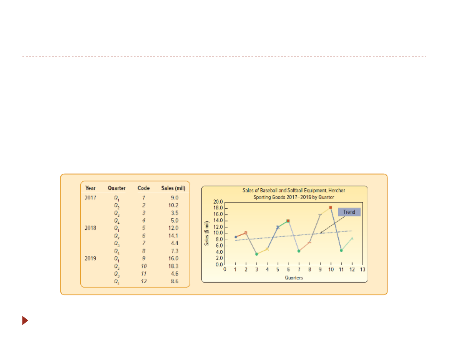
 Almost all businesses tend to have recurring seasonal patterns
 Men’s and women’s apparel have high sales right before
Christmas and low sales in January
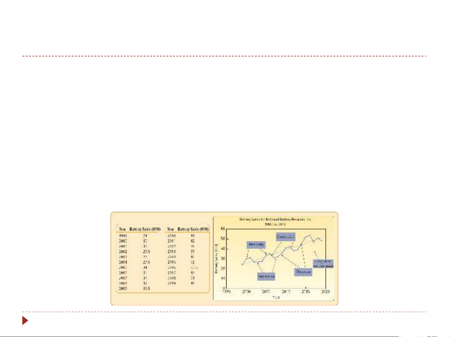
 Sporting good stores will have seasonal fluctuations 5-6 Cyclical Variation Example
 A typical business cycle consists of a period of prosperity
followed by periods of recession, depression, and then recovery
 In periods of recession, employment, production, the
DJIA, and other business and economic series are below the long-term trend lines
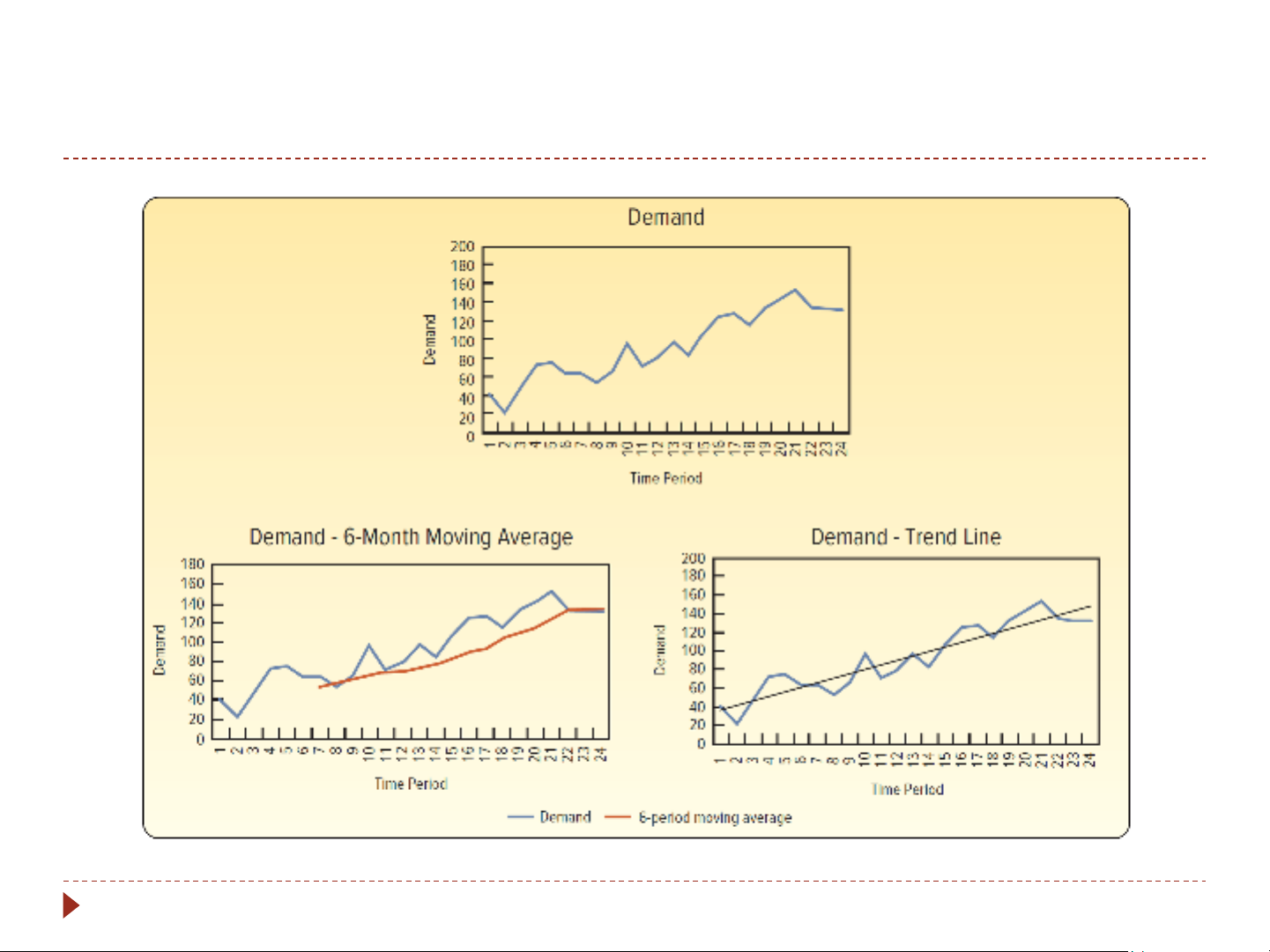
 In times of prosperity, they are above the long-term trend lines 5-7 Moving Averages
 A moving average is used to smooth the trend in a time series
 It is the basic method used in measuring seasonal fluctuation
 To apply a moving average, the data needs to follow a
fairly linear trend and have a rhythmic pattern of fluctuations
 This is accomplished by “moving” the mean values through the time series 5-8 Moving Average Example
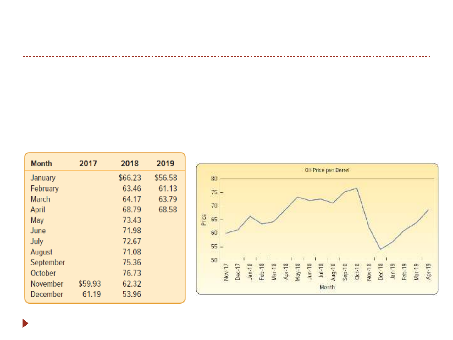
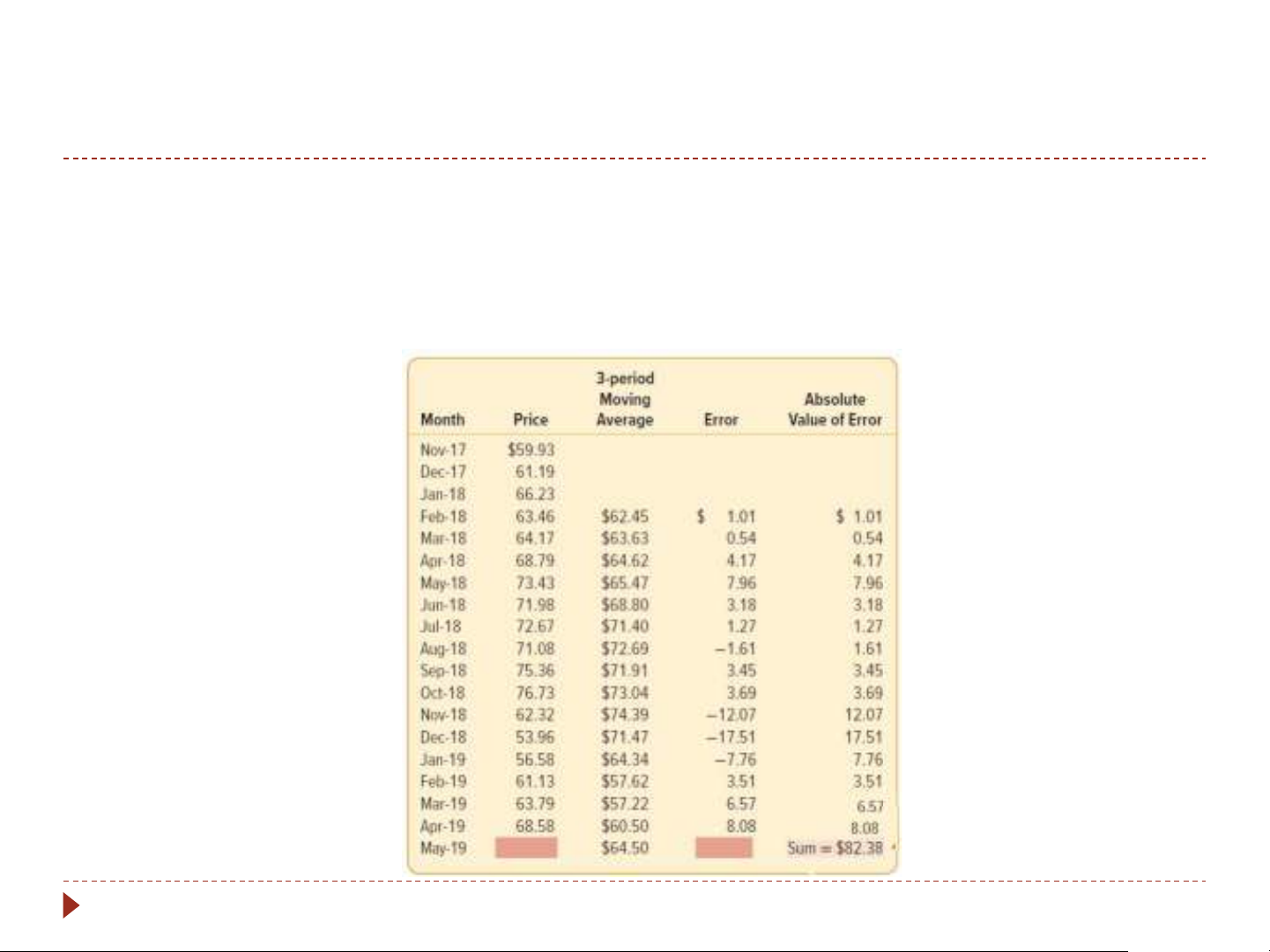
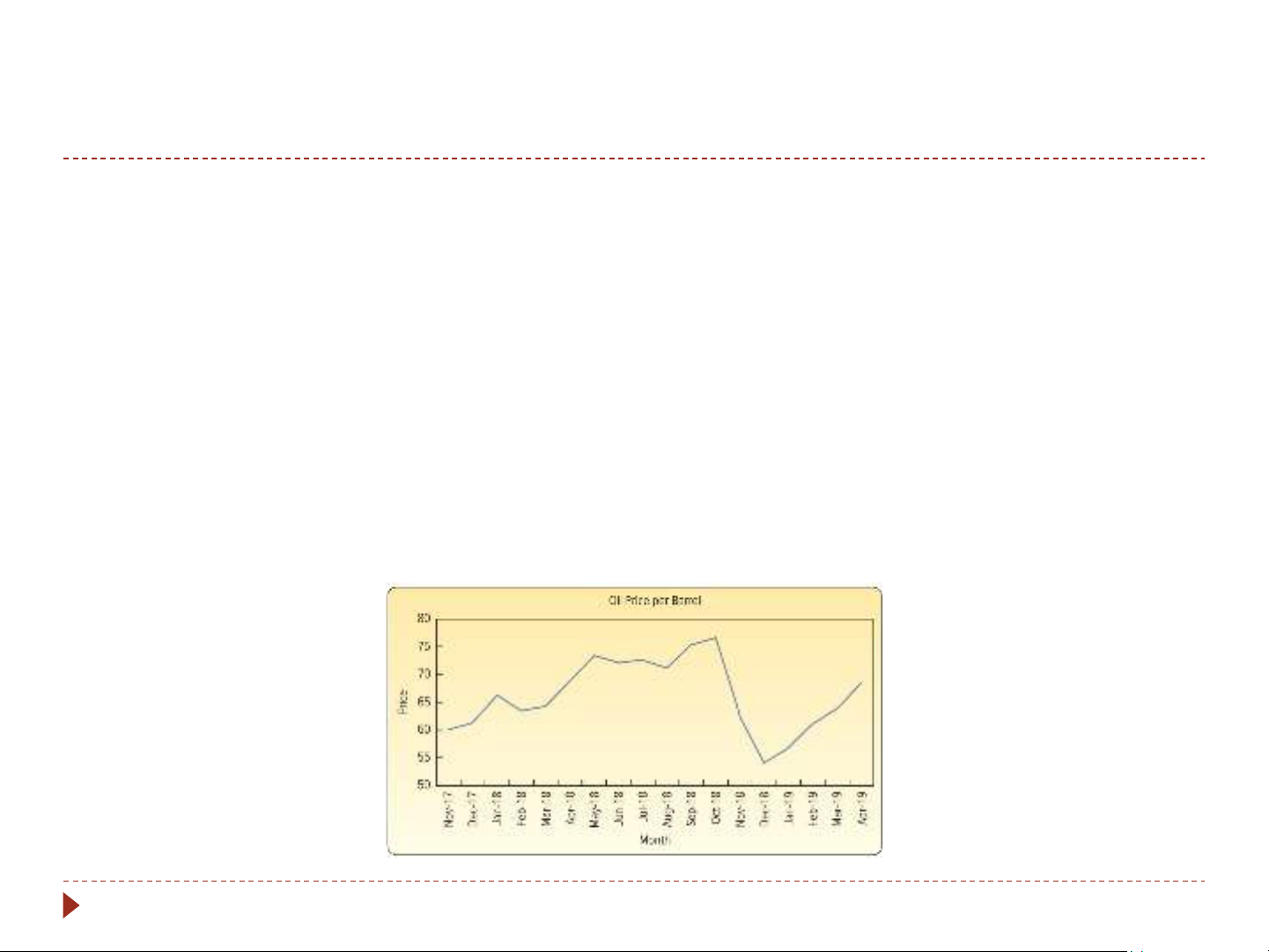
Shown is a time series of the monthly market price for a
barrel of oil over 18 months. Use a three-period and a six-
period simple moving average to forecast the oil price for May 2019. 5-9
3- and 6- Period Moving Average Example
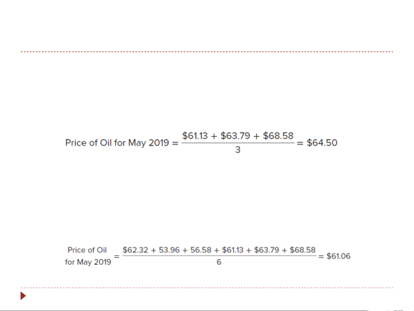
 Using a three-period simple moving average, the forecast for
May 2019 would be the average of the prices from the most
recent 3 months: February, March, and April of 2019. The
forecast is computed as follows:
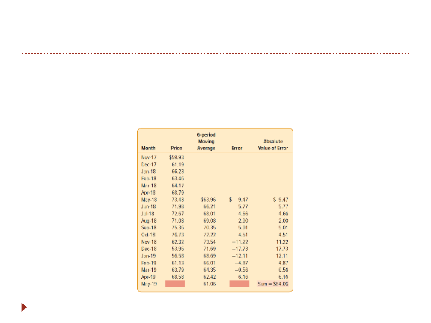
 Using a six-period simple moving average, the forecast for May
2019 would be the average of the prices from the most recent
6 months: November, December, January, February, March, and
April of 2019. The forecast is computed as follows: 5-10 Forecasting Error
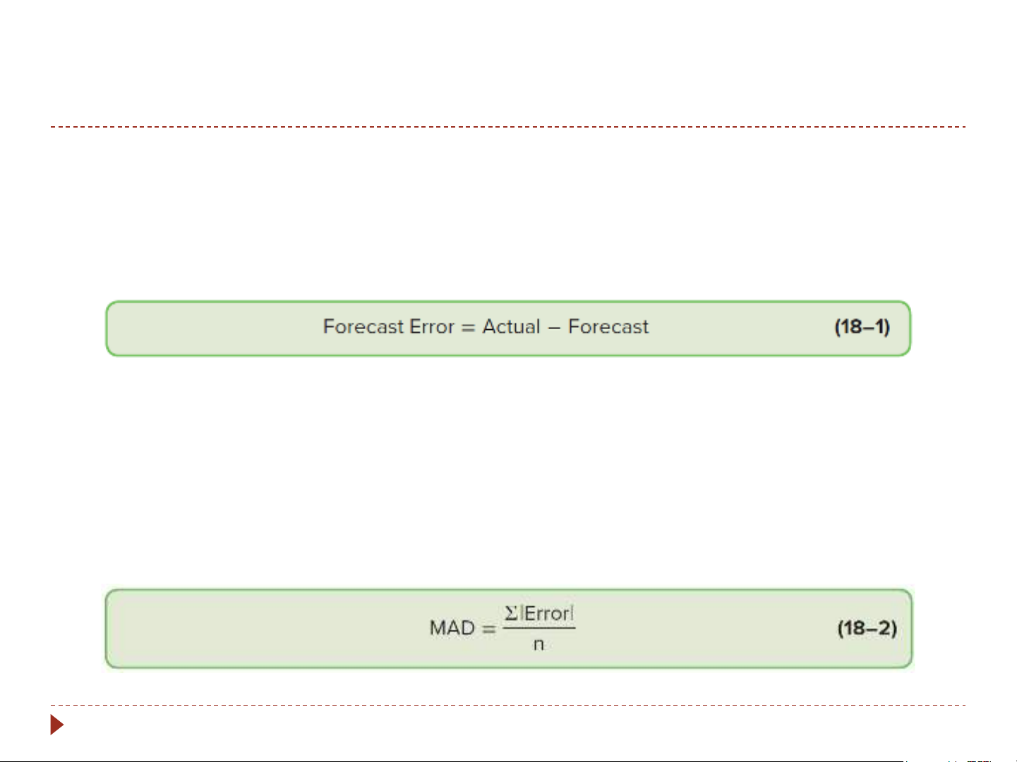
 Any estimate or forecast is likely to be imprecise. The
error, or lack of precision, is the difference between the
actual observation and the forecast.
 This difference is called a deviation of the forecast from the actual value.
 The mean of the absolute errors is called the mean absolute deviation (MAD). 5-11
3-Period Moving Average Including Error
 We report that the forecast for May 2019 is $64.50 with a MAD of $5.49.
Using a three-period simple moving average, we can expect the forecasted
May 2019 oil price to be between $59.01 (found by $64.50 − $5.49) and
$69.99 (found by $64.50 + $5.49). 5-12
6-Period Moving Average Including Error
 Using a 6-month moving average model, the MAD or the average variability
of forecast error is $7.01. Recalling that the 6-month moving average
forecast for May 2019 is $61.06, we can expect the forecasted May 2019 oil
price to be between $54.05 (found by $61.06 − $7.01) and $68.07 (found by $61.06 + $7.01). 5-13
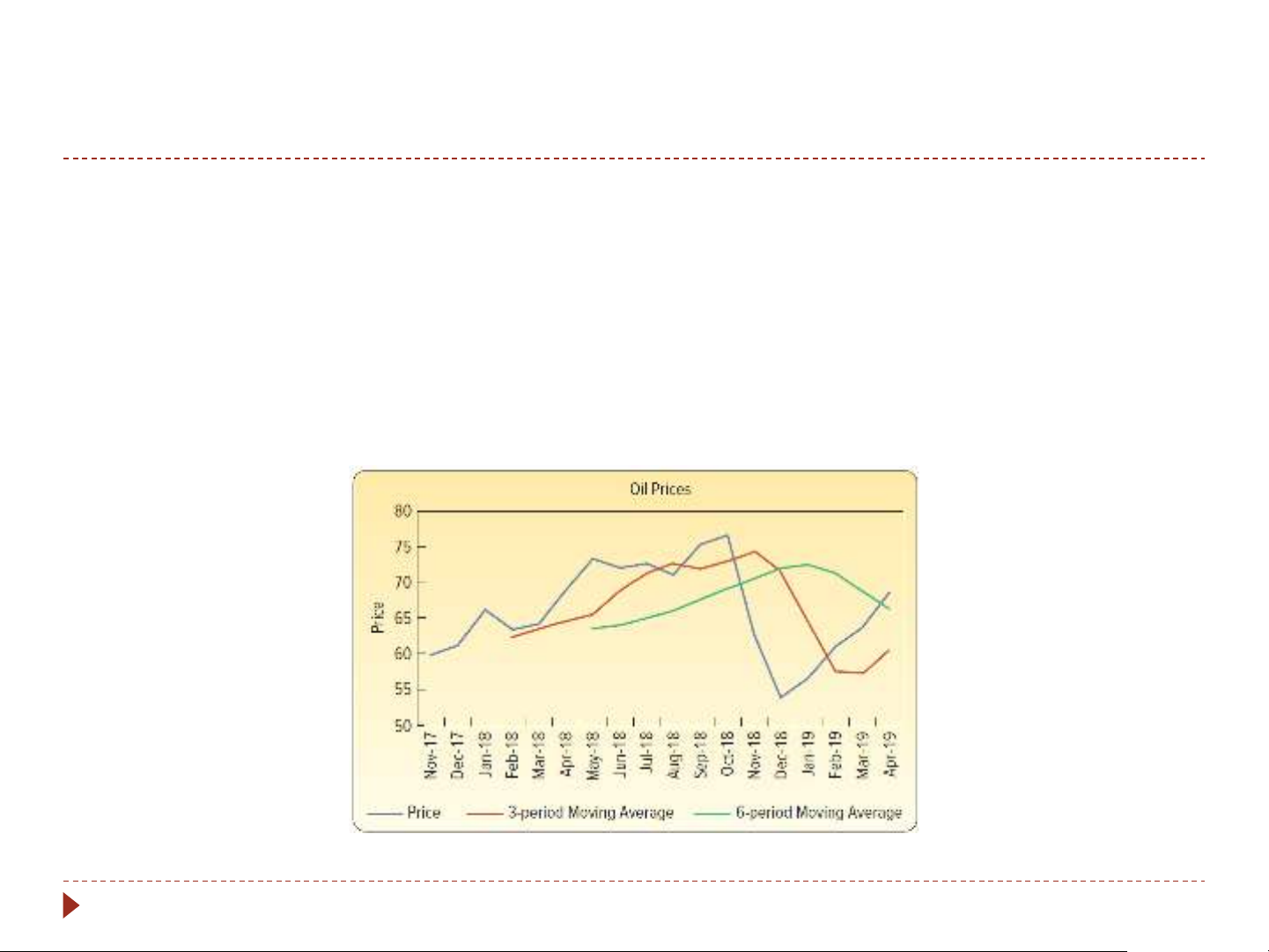
Simple Moving Average Comparison
 An outcome of using more periods in a simple moving average
is its effect on the variation of the forecasts.
 The variation in the forecasts is related to the number of
observations in a simple moving average. More periods will
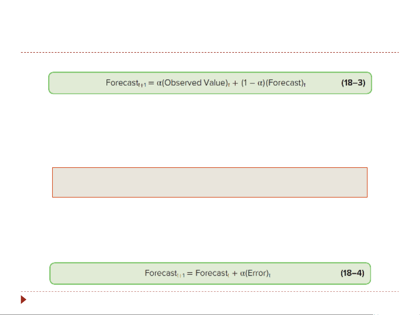
reduce the variation in the forecasts. 5-14 Simple Exponential Smoothing  t = time period  t+1 = next time period
 Alpha (α) = smoothing constant
SMOOTHING CONSTANT A value applied in exponential smoothing
to determine the weights assigned to past observations.
 Smoothing constant is between 0 and 1
 Selecting a smoothing constant value near 1 means that recent
data will receive more weight than older data. 5-15
Simple Exponential Smoothing Example
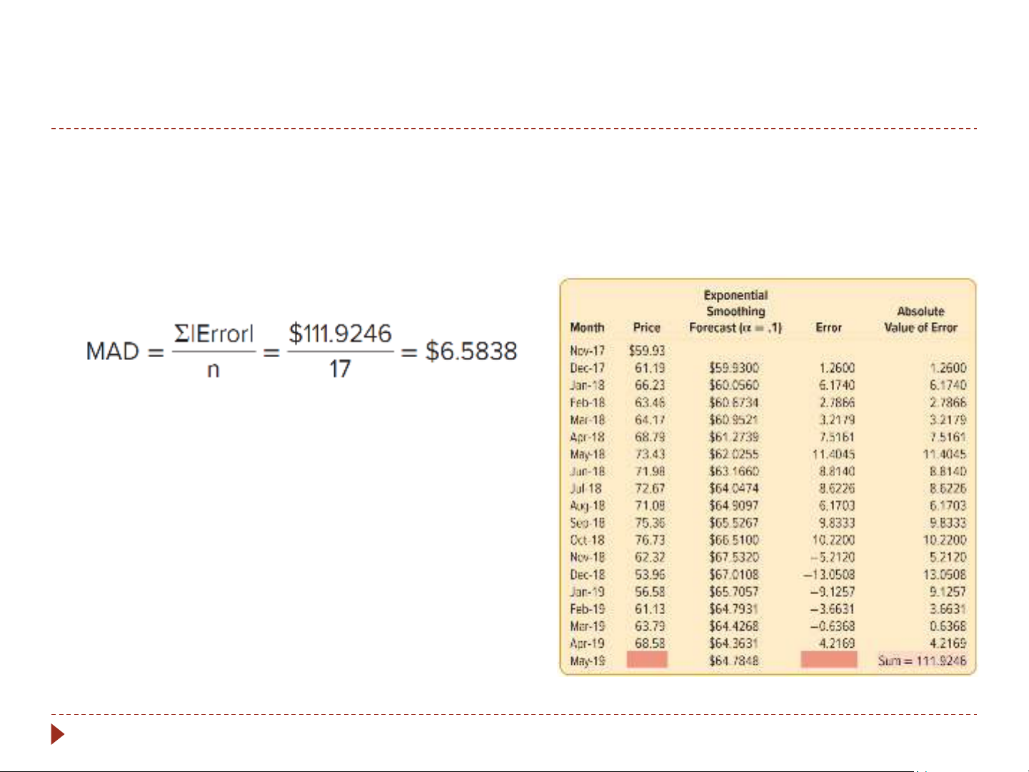
 Using simple exponential smoothing with a smoothing
constant of 0.1, the exponential smoothing equation would be:  Forecast = Forecast + 0.1(error) t+1 t t
 The forecast for January 2018 is:  Forecast = Forecast + 0.1(error) January December December Forecast
= $59.93 + 0.1($1.26) = $60.0560 January Forecast Error
= $66.23 − $60.06 = $6.1740 January 5-16
Simple Exponential Smoothing Example Continued
 The smoothing formula is applied through the time series
data until the last possible forecast for May 2019 is made.  MAD is then computed: 5-17
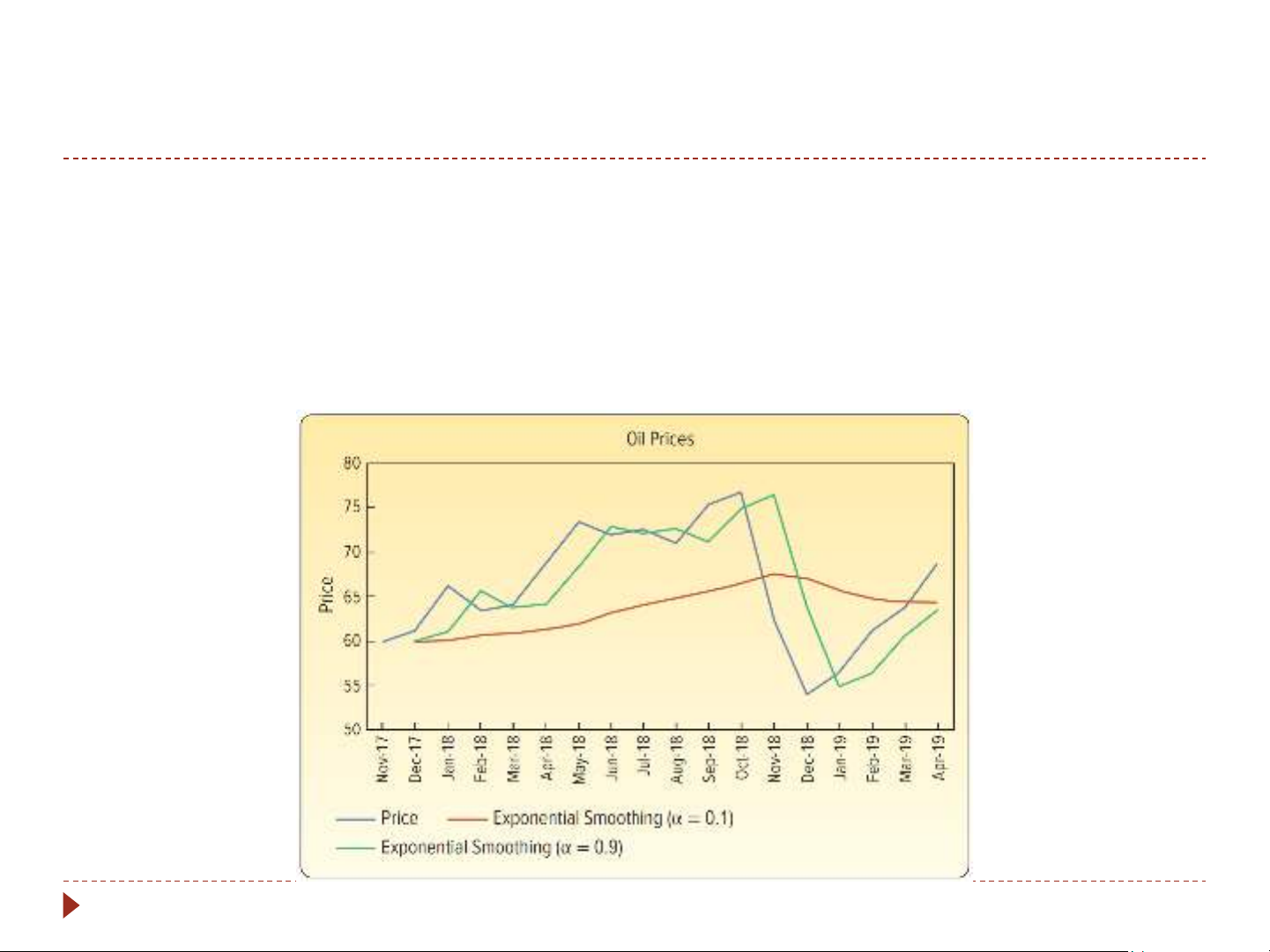
Simple Exponential Smoothing Example Concluded
 The forecast with the high alpha value, the green line graph, is
very responsive to the most recent oil price.
 The forecast with the low alpha value, the red line graph, is
much smoother and follows the average of oil prices over time. 5-18
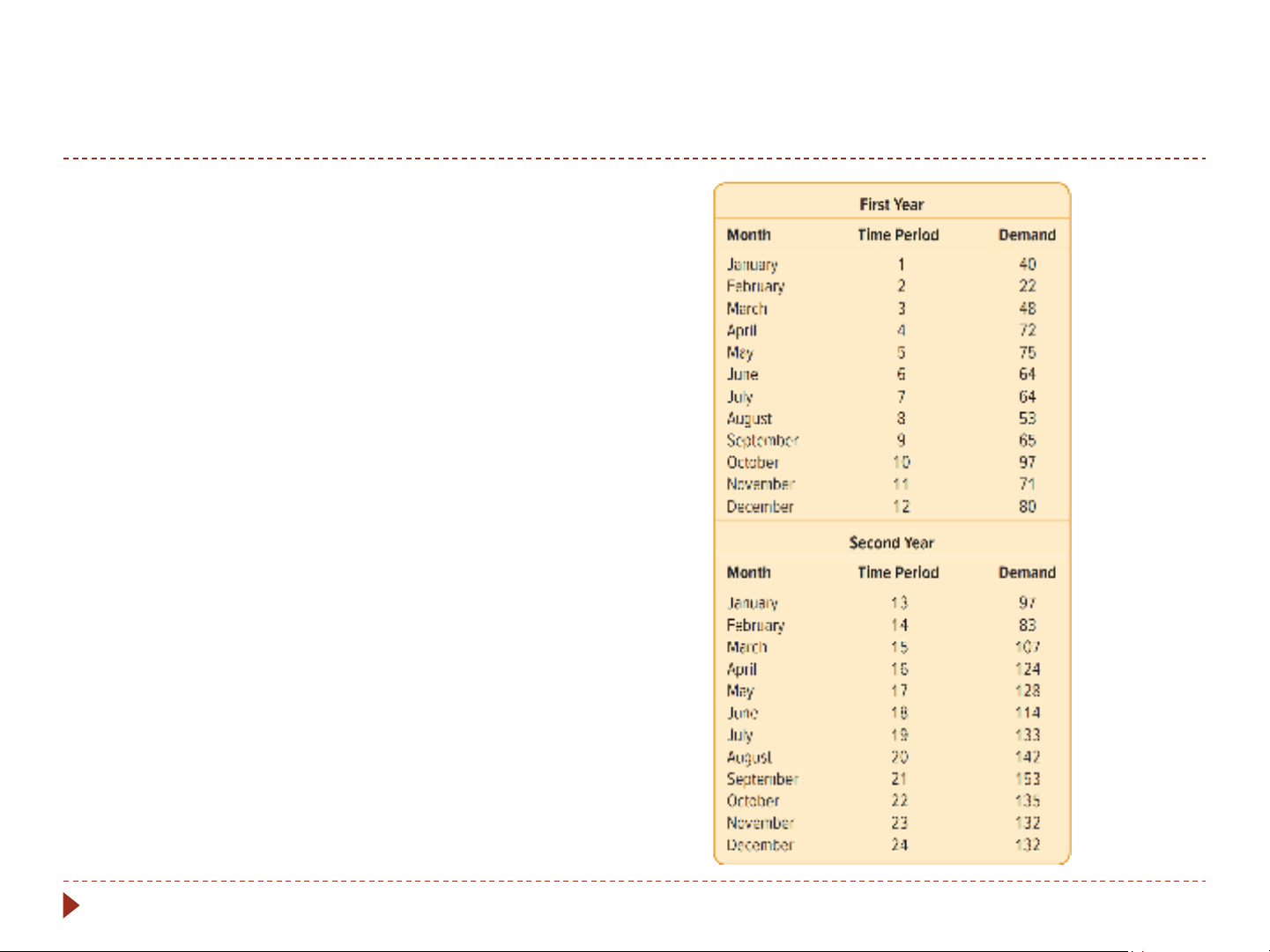
Time Series with a Trend: Regression Analysis  If the trend is linear, regression analysis is used to fit a linear trend model to the time series.  This time series is two years of monthly demand data. Each observation is labeled with the month. 5-19 Regression Analysis Example 5-20