Thống kê các ưng dụng của kinh tế

Statistic for economics and finance Instructor: Pham Ha Multiple Regression Analysis Chapter 4 4-1 Learning Objectives
LO4-1 Use multiple regression analysis to describe and interpret a
relationship between several independent variables and a dependent variable
LO4-2 Evaluate how well a multiple regression equation fits the data
LO4-3 Test hypothesis about the relationships inferred by a multiple regression model
LO4-4 Evaluate the assumptions of multiple regression
LO4-5 Use and interpret a qualitative, dummy variable in multiple regression
LO4-6 Include and interpret an interaction effect in multiple regression analysis
LO4-7 Apply stepwise regression to develop a multiple regression model
LO4-8 Apply multiple regression techniques to develop a linear model 4-2 Multiple Regression Analysis
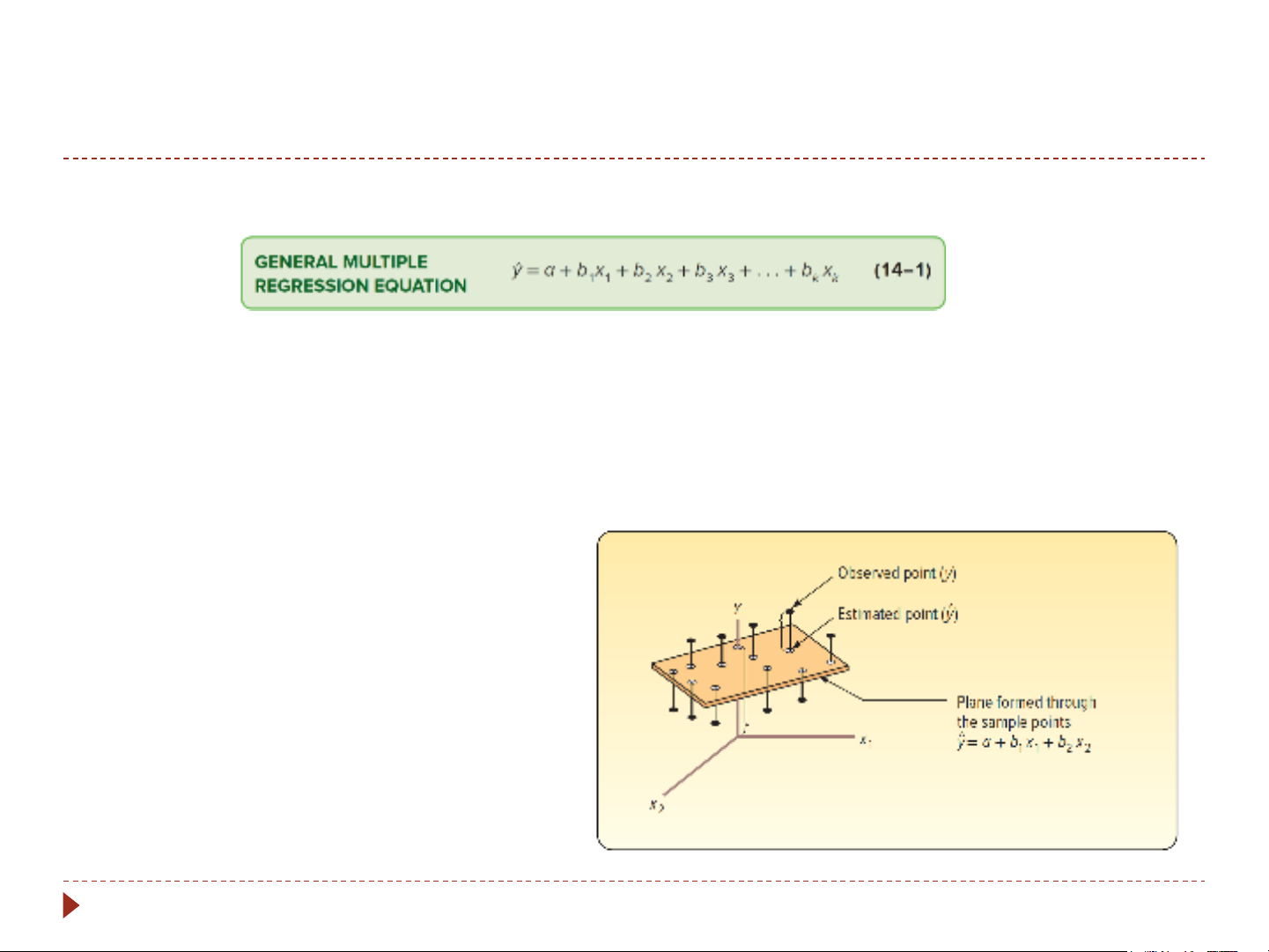
 The general form of a multiple regression formula is
 a is the intercept when all x’s are zero
 b refers to the sample regression coefficients
 x refers to the value of the various independent k variables  When there are two independent variables, the relationship can be graphically portrayed as a plane 4-3
Multiple Regression Analysis (2 of 2)
 The least squares criterion is used to develop the regression equation Example
 Suppose the selling price of a home is directly related to
the number of rooms and inversely related to its age, let
x refer to the number of rooms, x to the age of the 1 2
home and ොy to the selling price of the home ($000) ොy = 21.2 + 18.7x – .25x 1 2
ොy = 21.2 + 18.7(7) – .25(30) = 144.6
So, a seven-room house that is 30 years old is expected to sell for $144,600 4-4
Multiple Regression Analysis Example
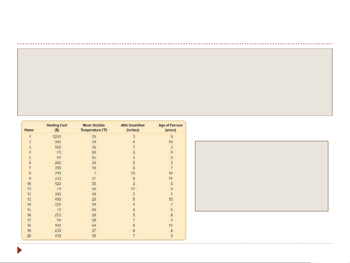
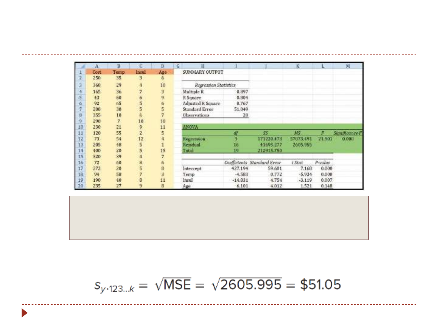
Salsberry Realty sells homes along the East Coast of the United States. One question
frequently asked by prospective buyers is “how much can we expect to pay to heat the
home in the winter”? The research department at Salsberry thinks 3 variables relate to
heating costs: the mean daily outside temperature, the number of inches of insulation,
and the age in years of the furnace. They conduct a random sample of 20 homes.
Determine the regression equation. y is the dependent variable x is the outside temperature 1 x is inches of insulation 2 x is the age of the furnace 3 ොy = a + b x +b x +b x 1 1 2 2 3 3
ොy is used to estimate the value of y 4-5
Multiple Regression Analysis Example (2 of 2)
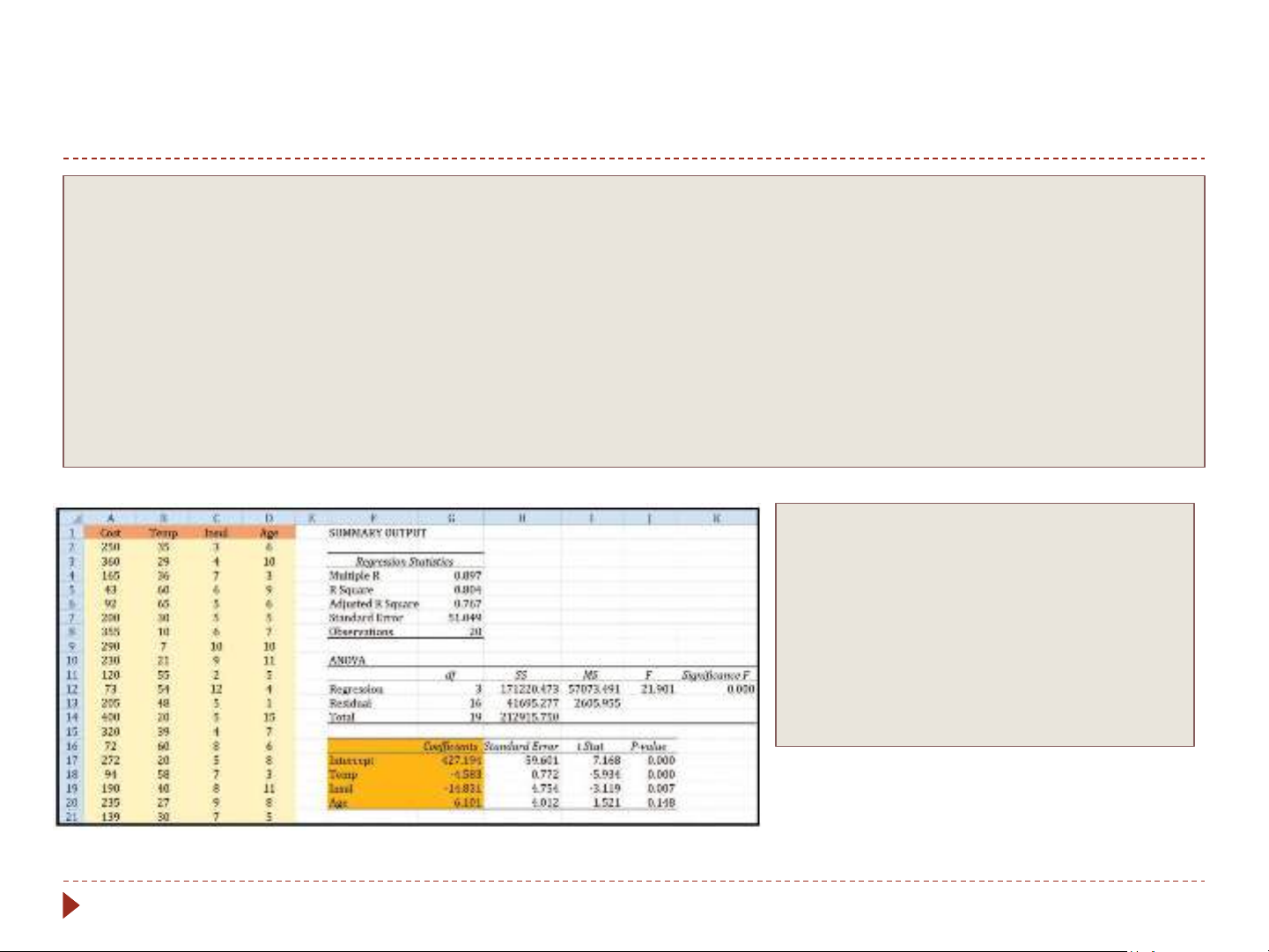
Once we determine the regression equation, we can calculate the heating costs for
January, given the mean outside temperature is 30 degrees, there are 5 inches of
insulation, and the furnace is 10 years old. ොy = a + b x +b x +b x 1 1 2 2 3 3
ොy = 427.194 – 4.583x – 14.831x + 6.101x 1 2 3
ොy = 427.194 - 4.583(30) – 14.831(5) + 6.101(10) = 276.56
Thus, the estimated heating costs for January are $276.56 Recall: y is the dependent variable x is the outside temperature 1 x is inches of insulation 2 x is the age of the furnace 3
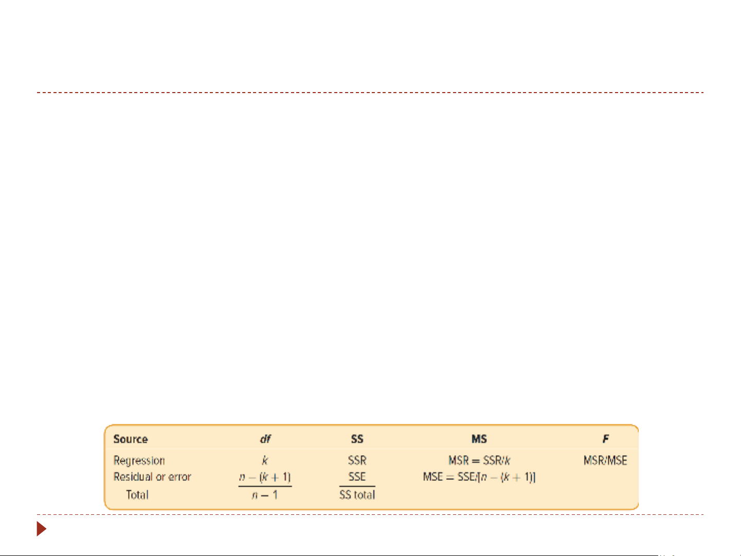
ොy is the estimated value of y 4-6 ANOVA Table
 An ANOVA table summarizes the multiple regression analysis
 It reports the total amount of the variation divided in two components
 The regression, the variation in all the independent variables
 The residual or error, the unexplained variation of y
 It reports the degrees of freedom of the independent
variables, the error variation, and the total variation 4-7 Measures of Effectiveness
 There are two measures of effectiveness of the regression equation
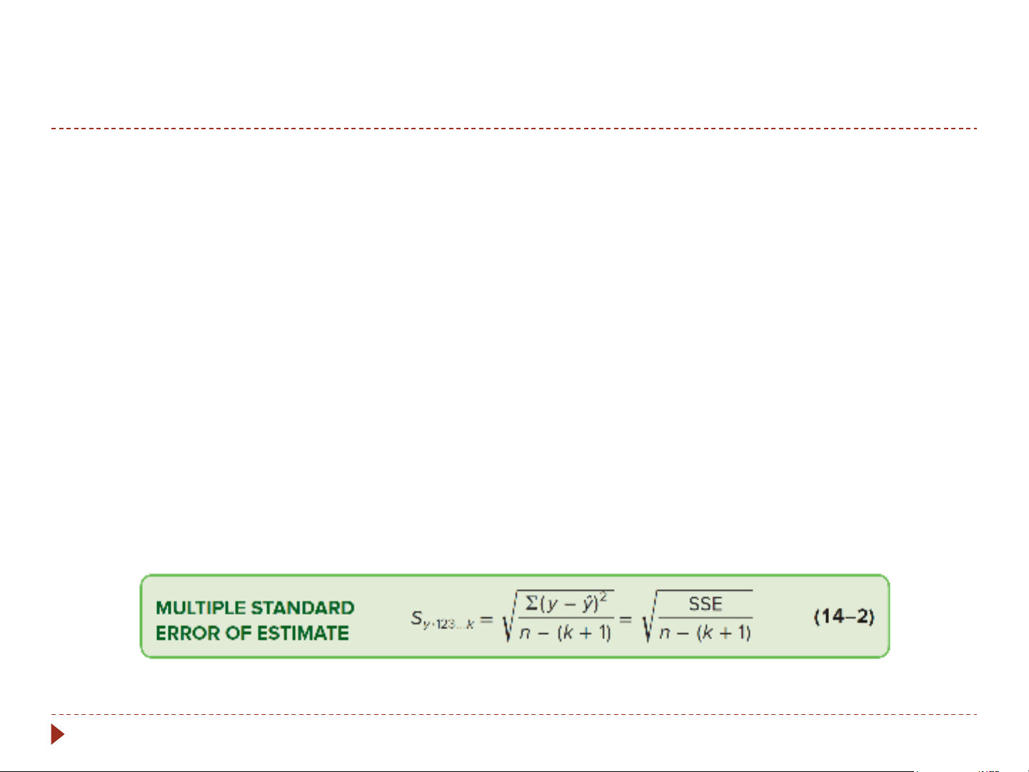
 The multiple standard error of the estimate is similar to the standard deviation
 It is measured in the same units as the dependent variable
 It is based on squared deviations between the observed and
predicted values of the dependent variable
 It ranges from 0 to plus infinity
 It is calculated from the following equation 4-8 ANOVA Table (2 of 2)
ොy = 427.194 – 4.583x – 14.831x + 6.101x 1 2 3
ොy = 427.194 – 4.583(35) – 14.831(3) + 6.101(6) = $258.90
Then, (y- ොy)2 = (250 – 258.90)2 = (8.90)2 = 79.21
Multiple Standard Error of the estimate 4-9
Measures of Effectiveness (2 of 3)
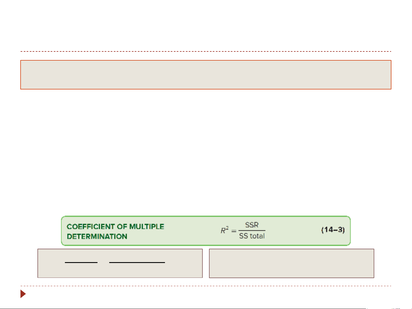
COEFFICIENT OF MULTIPLE DETERMINATION The percent of variation in the
dependent variable, y, explained by the set of independent variables, x , x , x , …x . 1 2 3 k
 The coefficient of multiple determination  Is symbolized by R2  Can range from 0 to 1
 Cannot assume negative values  Is easy to interpret
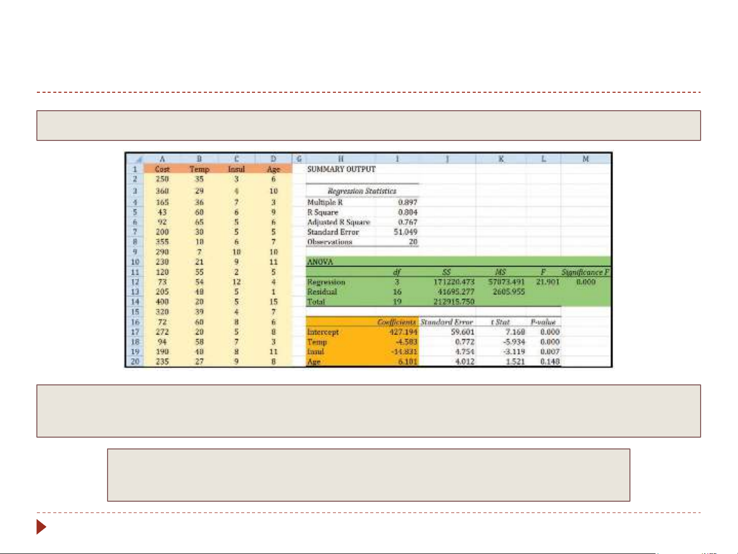
 It is found by the following formula SSR 171,220.473
R2 = SS total = 212,915.750 = .804
80.4% of the variation is explained by the 3 independent variables. 4-10
Measures of Effectiveness (3 of 3)
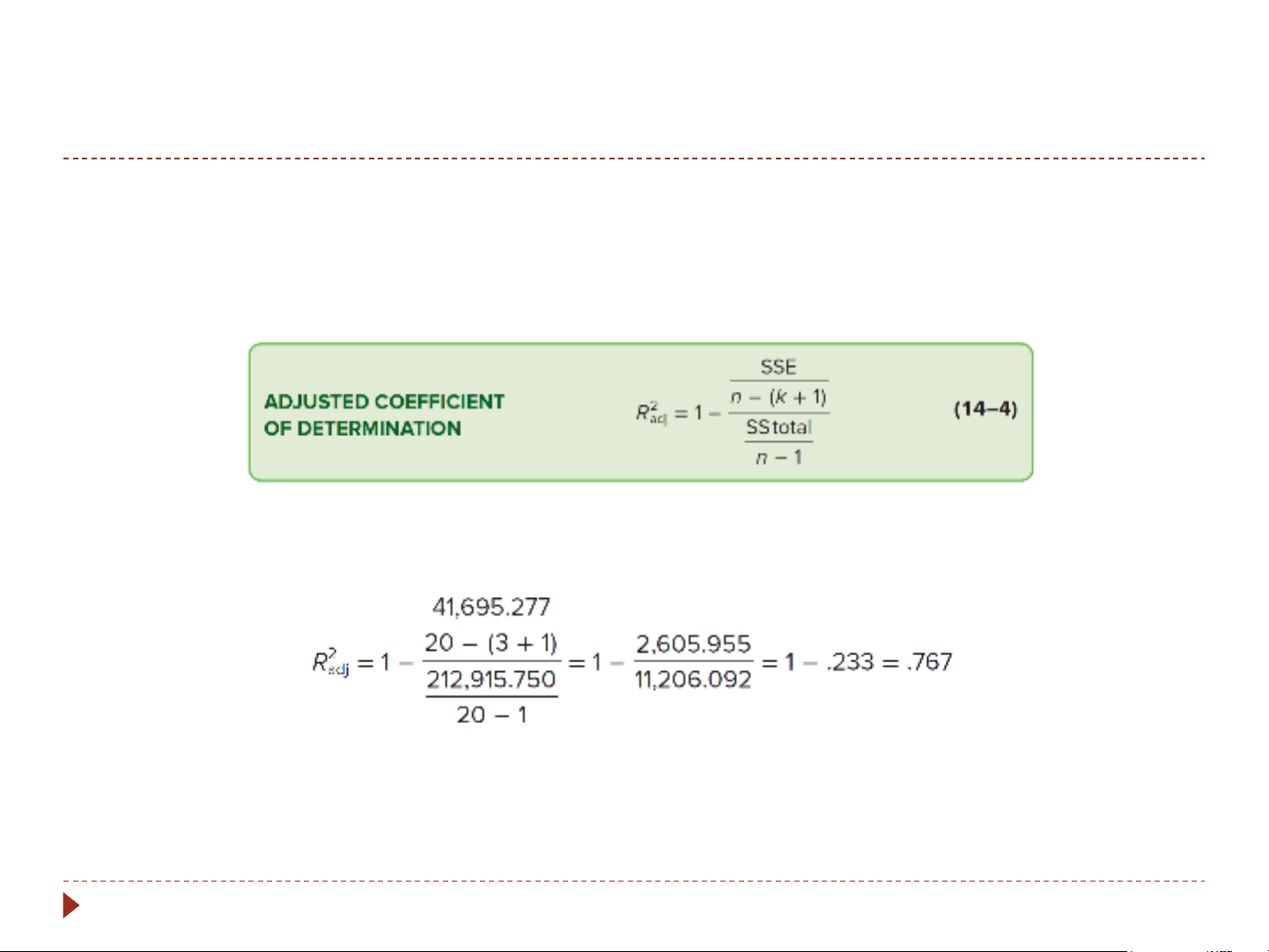
 When the number of independent variables is large, we
adjust the coefficient of determination for the degrees of freedom as follows
 For the cost of heating example, the adjusted coefficient of determination is
 If we compare R2 (0.80) to the adjusted R2 (0.767), the
difference in this case is small 4-11 Global Test
 A global test investigates whether it is possible that all the
independent variables have zero regression coefficients  The hypotheses are H : β = β = β = 0 0 1 2 3 H : Not all β are 0 1 is
 The test statistic is the F distribution
 There is a family of F distributions  It cannot be negative  It is continuous  It is positively skewed  It is asymptotic 4-12 Global Test (2 of 4)
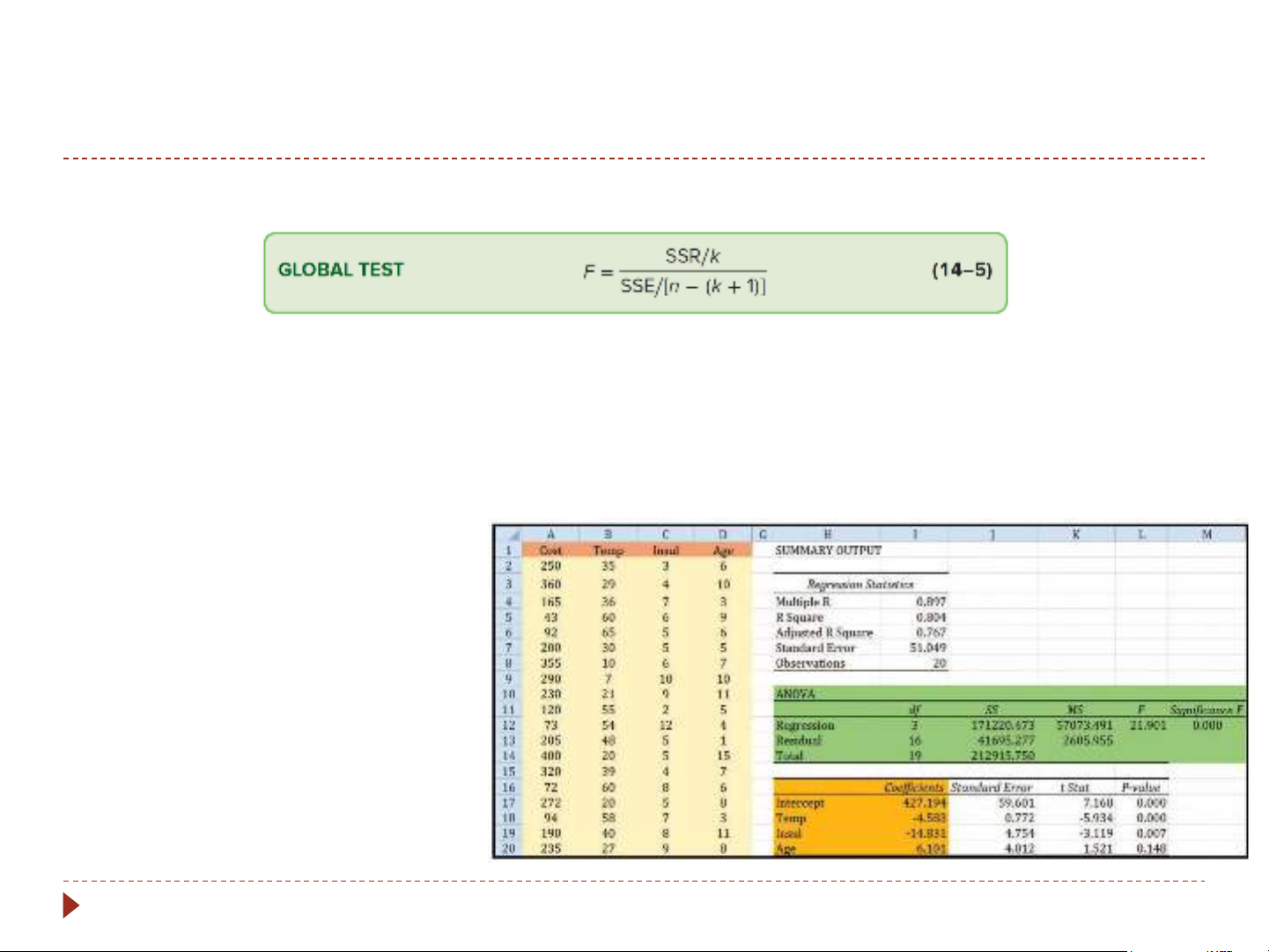
 The formula to calculate the value of the test statistic is
 with k (the number of independent variables) degrees of freedom in the numerator
 n – (k+1) degrees of freedom in the denominator  n is sample size  We can obtain the degrees of freedom from the ANOVA table 4-13 Global Test (3 of 4)
Step 1: State the null and the alternate hypothesis H : β = β = β = 0 0 1 2 3 H : Not all β are 0 1 is
Step 2: Select the level of significance, we’ll use .05
Step 3: Select the test statistic, F
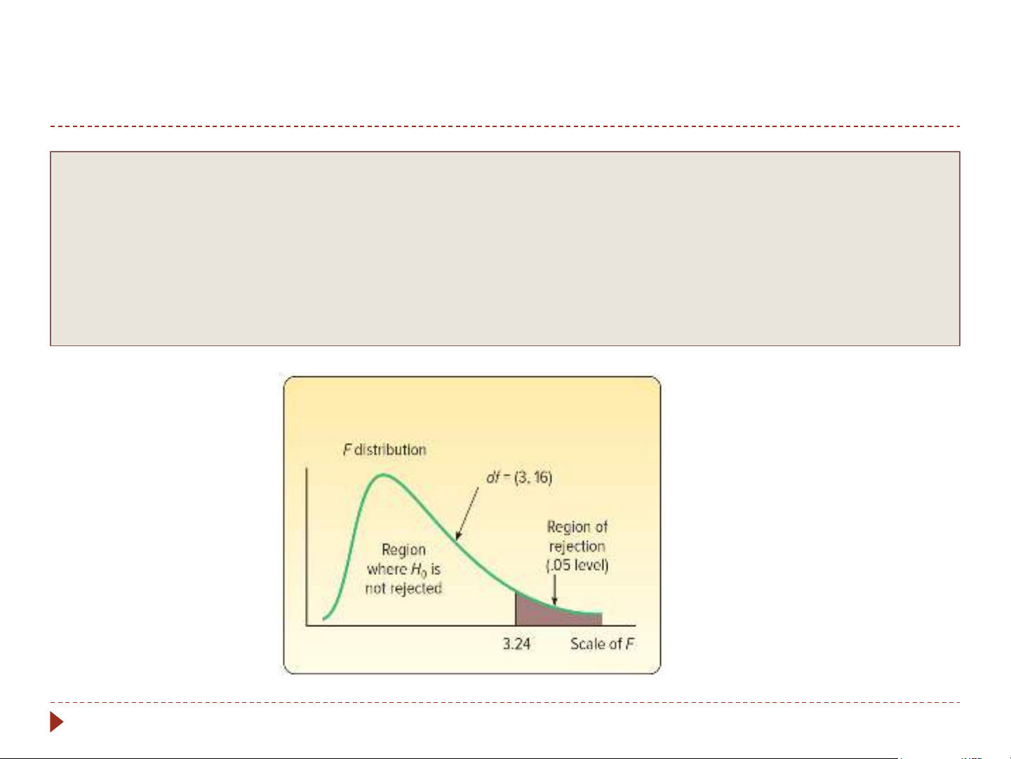
Step 4: Formulate the decision rule, reject H if F > 3.24 0 4-14 Global Test (4 of 4)
Step 5: Make decision; reject H , F=21.90 0
Step 6: Interpret; at least one of the independent variables has the ability to explain the variation in heating cost.
The global test assures us that outside temperature, the amount of
insulation, or the age of the furnace has a bearing on heating cost! 4-15 Test for Individual Variables
 The test for individual variables determines which
independent variables have regression coefficients that differ significantly from zero
 The variables that have zero regression coefficients are
usually dropped from the analysis
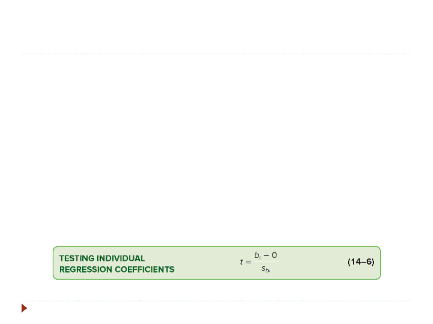
 The test statistic is the t distribution with n – (k +1) degrees of freedom
 The formula to calculate the value of the test statistic for the individual test is 4-16
Evaluating Individual Regression Coefficients Example
Salsberry Realty will use three sets of hypothesis: one for temperature, one for
insulation, and one for age of the furnace.
Step 1: State the null and alternate hypothesis For temperature b H : β 1−0 0 1 = 0 t = = −4.583−0 H : β s 0.722 = − 5.937 1 1 ≠ 0 b1 For insulation b H : β 2−0 0 2 = 0 t = s = −14.831−0 4.754 = − 3.119 H : β b2 1 2 ≠ 0 For furnace age b H : β 3−0 0 3 = 0 t = s = 6.101−0 4.012 = 1.521 H : β ≠ 0 b3 1 3
Step 2: Select the level of significance; we use .05
Step 3: Select the test statistic; we’ll use t
Step 4: Formulate the decision rule, reject H if t < −2.120 or > 2.120 0
Step 5: Make decision; reject H for temperature and insulation but not furnace age 0
Step 6: Interpret; furnace age is not a significant predictor of heating costs 4-17
Evaluating Individual Regression Coefficients Example (2 of 2)
Salsberry Realty will rerun the regression equation using temperature and insulation.
ොy = 490.286 – 5.150x – 14.718x 1 2
The hypotheses and details of the global test are, reject the null hypothesis if F > 3.59 H : β = β = 0 0 1 2
H : Not all of the β ’s are equal 1 1 SSR−k F = SSE/(n−(k+1) = 165,194.521/2
47,721.229/(20− 2+1 ) = 29.424 For temperature b H : β 1−0 0 1 = 0 t = s = −5.150−0 0.702 = − 7.337 H : β b1 1 1 ≠ 0 For insulation b H : β 2−0 0 2 = 0 t = s = −14.718−0 4.934 = − 2.983 H : β b2 1 2 ≠ 0
Step 2: Select the level of significance; we use .05
Step 3: Select the test statistic; we’ll use t
Step 4: Formulate the decision rule, reject H if t < −2.110 or > 2.110 0
Step 5: Make decision; reject H for temperature and insulation 0
Step 6: Interpret; temperature and insulation are a significant predictor of heating costs 4-18
Multiple Regression Assumptions
 There are five assumptions to use multiple regression analysis 1. There is a linear relationship 2.
The variation in the residuals is the same for both large and small values of ොy 3.
The residuals follow the normal distribution 4.
The independent variable should not be correlated 5. The residuals are independent
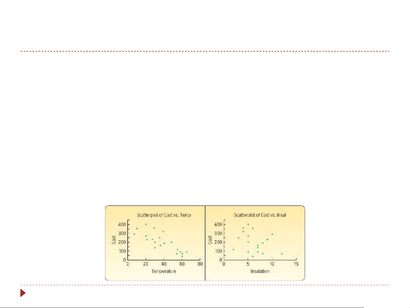
 Next, we’ll provide a brief discussion of each of these assumptions. 4-19 Linear Relationship Assumption
 The relationship between the dependent variable and the
set of independent variables must be linear
 To verify this assumption, develop a scatter diagram and
plot the dependent variable on the vertical axis and the
independent variable on the horizontal axis
 The plots below indicate a fairly strong negative
relationship between temperature and heating cost and
negative relationship between insulation and costs 4-20