Ch2_Statistical_Learning- Tài liệu xác suất thống kê
Ch2_Statistical_Learning- Tài liệu xác suất thống kê. Tài liệu tổng hợp được sưu tầm gồm 37 trang. Mời các bạn tham khảo
Môn: Xác suất thống kê và quy hoạch thực nghiệm 34 tài liệu
Trường: Đại học Bách Khoa Hà Nội 5.7 K tài liệu
Tác giả:


Preview text:
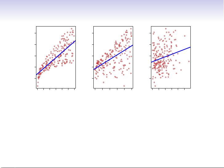
What is Statistical Learning? 25 25 25 20 20 20 15 15 15 Sales Sales Sales 10 10 10 5 5 5 0 50 100 200 300 0 10 20 30 40 50 0 20 40 60 80 100 TV Radio Newspaper
Shown are Sales vs TV, Radio and Newspaper, with a blue
linear-regression line fit separately to each.
Can we predict Sales using these three?
Perhaps we can do better using a model
Sales ≈ f(TV, Radio, Newspaper) 1 / 30 Notation
Here Sales is a response or target that we wish to predict. We
generically refer to the response as Y .
TV is a feature, or input, or predictor; we name it X1.
Likewise name Radio as X2, and so on.
We can refer to the input vector collectively as X 1 X = X2 X3 Now we write our model as Y = f (X) +
where captures measurement errors and other discrepancies. 2 / 30 What is f (X) good for?
• With a good f we can make predictions of Y at new points X = x.
• We can understand which components of
X = (X1, X2, . . . , Xp) are important in explaining Y , and
which are irrelevant. e.g. Seniority and Years of
Education have a big impact on Income, but Marital Status typically does not.
• Depending on the complexity of f , we may be able to
understand how each component Xj of X affects Y . 3 / 30 ●● 6 ● ● ● ● ● ● ● ● ● ●● ● ● ● 4 ●● ● ●● ● ●● ● ●●● ● ● ● ● ● ● ●● ● ●● ● ● ●● ● ● ● ● ● ● ●● ● ● ● ● ● ● ● ● ●● ● ● ● ● ● ● ● ● ● ● ● ● ● ● ● ● ● ● ● ● ● ● ● ● ● ●● ● ● ● ● ●● ● ● ● ● ● ● ● ● ● ● ● ● ● ● ● ● ● ● ● ● ● y ● ● ● ● ● ● ● ● ● ● ●● ● ● ● ●● ● 2 ● ●●● ● ● ● ● ● ● ● ● ● ● ● ●● ● ●● ● ● ● ●● ● ● ● ● ● ● ● ● ● ● ● ● ● ●● ● ● ● ● ● ● ● ●● ● ● ● ● ● ● ● ● ● ● ●● ● ● ● ● ● ● ● ● ●● ● ● ● ● ● ●● ● ● ● ● ● ●● ● ● ● ● ● ● ● ● ● ● ● ● ● ● ● ● ●● ● ● ● ● ●● ● ●● ●● ● ● ● ● ● ● ● ● ● ● ● ● ● ● ● ● ● ● ● ● ● ● ● ● ● ● ● ● ● ● ● ● ● ● ● ● ● ● ●●● ● ● ● ● ● ● ● ● ● ●● ● ● ● ● ● ● ● ● ●● ●● ● ●● ●● ● ● ●● ● ● ● ● ● ● ● ● ● ●● ● ● ● ● ● ● ● ● ● ● ● ● ● ● ● ● ● ● ● ● ● ● ● ● ● ● ● ● ●●● ● ● ● ● ● ● ● ● ● ● ● ● ● ● ● ● ● ● ● ● ● ●● ● ●●●● ●● ● ● ● ● ● ● ● ● ● ● ● ● ● ● ●● ● ● ●● ● ●● ● ● ● ● ● ● ●● ● ● ● ● ● ●● ● ● ● ● ● ● ● ● ● ● ● ● ● ● ●● ● ● ● ● ● ● ● ● ● ● ● ● ● ● ● ● ● ● ● ● ● ● ●● ● ● ● ● ● ● ●●● ● ● ● ● ●● ● ● ● ● ● ● ● ● ● ● ● ● ● ● ● ● ● ● ● ● ● ● ● ● ● ● ● ● ● ● ● ● ● ● ● ● ● ● ● ● ● ●● ● ●● ● ● ● ● ● ● ● ● ● ● ● ● ●● ● ● ● ● ● ● ● ● ● ● ● ● ● ● ● ● ● ● ● ● ● ● ●● ● ● ● ● ● ● ●● ● ● ● ● ● ● ● ● ● ● ● ●● ● ● ●● ● ● ● ● ● ●● ● ● ● ● ● ● ● ● ●● ● ● ● ● ● ● ● ● ● ● ● ● ● ● ● ● ● ● ● ● ● ● ● ● ●● ● ● ● ● ● ● ●● ● ● ● ● ● ● ● ● ● ● ● ● ● ● ● ● ● ● ● ● ● ● ● ● ●● ● ● ●●● ● ● ● ● ● ● ● ● ● ● ● ● ● ● ● ● ● ● ● ● ● ● ● ● ● ● ● ● ●● ● ● ● ● ● ● ●● ● ● ● ● ● 0 ● ● ● ● ● ● ●● ●● ● ● ● ● ● ● ● ● ● ● ● ● ●● ● ● ●● ● ● ● ● ● ● ● ● ● ● ● ● ● ● ● ● ● ● ● ● ● ● ● ● ● ● ● ●● ● ● ● ●● ● ●● ● ● ● ●● ● ● ● ● ● ● ● ● ● ● ● ● ● ●● ● ● ● ● ● ● ● ● ● ● ● ● ● ● ● ● ● ● ● ● ● ● ● ● ● ● ● ●● ● ● ● ● ● ● ● ● ● ●● ● ● ● ● ● ● ● ● ●●●● ● ● ● ● ● ● ● ● ● ● ●● ● ● ● ● ●● ● ● ● ●● ● ● ● ●
●● ● ● ● ●● ● ● ● ● ● ● ● ● ● ● ● ● ● ● ● ● ● ● ● ●● ●● ● ● ● ● ● ● ● ● ● ● ● ● ● ●● ● ● ● ●● ● ● ● ● ● ● ● ● ● ●● ● ● ● ● ● ● ● ● ● ● ● ● ●●● ● ● ● ● ● ● ● ● ● ● ● ● ● ● ● ● ● ● ● ● ● ● ●●●● ●● ● ● ● ● ● ● ●● ● ●● ● ● ● ●●● ●● ● ● ● ● ● ● ● ● ● ● ● ●● ● ●● ● ● ● ● ● ● ● ● ● ● ● ● ● ● ●● ● ● ●●● ● ● ●● ● ●● ● ● ● ● ● ● ● ● ● ● ●● ● ● ● ● ● ● ●● ● ● ● ● ● ● ● ●●● ● ● ● ● ●● ● ● ● ● ●● ● ● ● ●● ● ● ● ● ● ● ● ●● ● ● ● ● ● ● ● ● ● ● ● ● ● ● ● ● ● ● ● ● ● ● ● ● ● ● ● ● ●● ● ● ● ● ● ● ● ● ●● ●● ● ● ● ● ● ● ● ● ●● ● ● ● ● ● ● ● ● ●● ● ● ● ● ● ● ● ● ● ● ● ●● ● ● ● ● ● ● ● ● ● ● ● ●●● ● ● ● ● ● ● ● ●● ● ●●● ● ● ● ● ● ●● ● ● ● ● ● ● ● ●● ● ● ● ● ● ● ● ● ● ● ● ● ● ● ● ● ● ● ● ● ● ● ●● ●● ● ● ● ● ● ● ● ● ●● ● ● ●● ● ● ● ● ● ● ● ● ● ● ●● ● ● ● ● ● ●● ● ● ● ● ● ● ● ● ●● ● ● ● ● ● ● ● ● ● ● ● ● ● ● ● ● ● ● ● ● ● ●● ● ● ●● ● ● ● ● ● ● ● ● ● ● ● ● ● ● ● ● ● ● ● ● ● ● ● ● ●●● ● ● ● ● ● ● ● ● ● ● ●● ● ● ● ● ● ● ● ● ● ● ● ● ● ● ● ● ● ●●● ● ● ● ●● ● ● ● ● ● ● ● ● ● ● ● ● ● ●● ● ● ● ● ● ● ● ●●● ● ● ● ● ●● ● ● ● ● ● ● ●● ●● ● ● ● ● ● ● ●● ● ● ● ● ● ● ● ● ● ● ● ● ● ● ● ● ● ● ● ● ● ● ● ● ● ● ● ● ● ● ● ● ● ● ● ● ● ● ● ● ● ● ● ● ● ● ● ● ● ● ● ● ● ● ● ● ● ●● ● ●● ● ●● ● ●● ● ● ● ● ● ● ● ● ● ● ● ● ●●● ● ● ● ● ● ● ● ● ● ● ● ● ● ● ● ● ● ● ● ● ● ● ● ●● ● ● ● ● ● ● ● ● ● ● ● ● ● ● ● ●● ● ● ● ● ● ● ● ● ● ● ● ● ● ● ● ● ● ● ● ● ● ● ● ● ● ● ● ●● ● ● ● ● ● ● ● ● ● ● ●● ● ●● ● ● ● ● ● ● ●● ●● ● ● ● ●● ● ● ● ● ●● ● ● ● ● ● ● ● ● ●● ● ● ● ● ● ● ●● ● ● ● ● ● ● ● ● ● ● ● ● ● ● ● ● ● ● ● ● ●● ● ● ●● ● ● ● ● ● ● ● ● ● ● ● ● ● ● ● ● ●● ● ● ● ● ● ● ● ● ● ● ● ● ● ●● ● ● ● ● ● ● ● ● ● ● ● ● ● ●● ● ● ● ● ● ●● ● ● ● ● ● ● ● ● ● ● ● ● ● ●● ● ● ● ● ● ● ● ● ● ● ● ● ●● ● −2 1 2 3 4 5 6 7 x
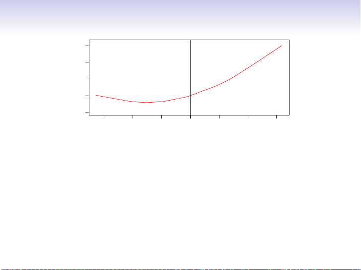
Is there an ideal f (X)? In particular, what is a good value for
f (X) at any selected value of X, say X = 4? There can be
many Y values at X = 4. A good value is f (4) = E(Y |X = 4)
E(Y |X = 4) means expected value (average) of Y given X = 4.
This ideal f (x) = E(Y |X = x) is called the regression function. 4 / 30
• Is the ideal or optimal predictor of Y with regard to
mean-squared prediction error: f (x) = E(Y |X = x) is the
function that minimizes E[(Y − g(X))2|X = x] over all
functions g at all points X = x.
• = Y − f(x) is the irreducible error — i.e. even if we knew
f (x), we would still make errors in prediction, since at each
X = x there is typically a distribution of possible Y values. • For any estimate ˆ f (x) of f (x), we have E[(Y − ˆ f (X))2|X = x] = [f(x) − ˆ f (x)]2 + Var() | {z } | {z } Reducible Irreducible The regression function f (x)
• Is also defined for vector X; e.g.
f (x) = f (x1, x2, x3) = E(Y |X1 = x1, X2 = x2, X3 = x3) 5 / 30
• = Y − f(x) is the irreducible error — i.e. even if we knew
f (x), we would still make errors in prediction, since at each
X = x there is typically a distribution of possible Y values. • For any estimate ˆ f (x) of f (x), we have E[(Y − ˆ f (X))2|X = x] = [f(x) − ˆ f (x)]2 + Var() | {z } | {z } Reducible Irreducible The regression function f (x)
• Is also defined for vector X; e.g.
f (x) = f (x1, x2, x3) = E(Y |X1 = x1, X2 = x2, X3 = x3)
• Is the ideal or optimal predictor of Y with regard to
mean-squared prediction error: f (x) = E(Y |X = x) is the
function that minimizes E[(Y − g(X))2|X = x] over all
functions g at all points X = x. 5 / 30 • For any estimate ˆ f (x) of f (x), we have E[(Y − ˆ f (X))2|X = x] = [f(x) − ˆ f (x)]2 + Var() | {z } | {z } Reducible Irreducible The regression function f (x)
• Is also defined for vector X; e.g.
f (x) = f (x1, x2, x3) = E(Y |X1 = x1, X2 = x2, X3 = x3)
• Is the ideal or optimal predictor of Y with regard to
mean-squared prediction error: f (x) = E(Y |X = x) is the
function that minimizes E[(Y − g(X))2|X = x] over all
functions g at all points X = x.
• = Y − f(x) is the irreducible error — i.e. even if we knew
f (x), we would still make errors in prediction, since at each
X = x there is typically a distribution of possible Y values. 5 / 30 The regression function f (x)
• Is also defined for vector X; e.g.
f (x) = f (x1, x2, x3) = E(Y |X1 = x1, X2 = x2, X3 = x3)
• Is the ideal or optimal predictor of Y with regard to
mean-squared prediction error: f (x) = E(Y |X = x) is the
function that minimizes E[(Y − g(X))2|X = x] over all
functions g at all points X = x.
• = Y − f(x) is the irreducible error — i.e. even if we knew
f (x), we would still make errors in prediction, since at each
X = x there is typically a distribution of possible Y values. • For any estimate ˆ f (x) of f (x), we have E[(Y − ˆ f (X))2|X = x] = [f(x) − ˆ f (x)]2 + Var() | {z } | {z } Reducible Irreducible 5 / 30 How to estimate f
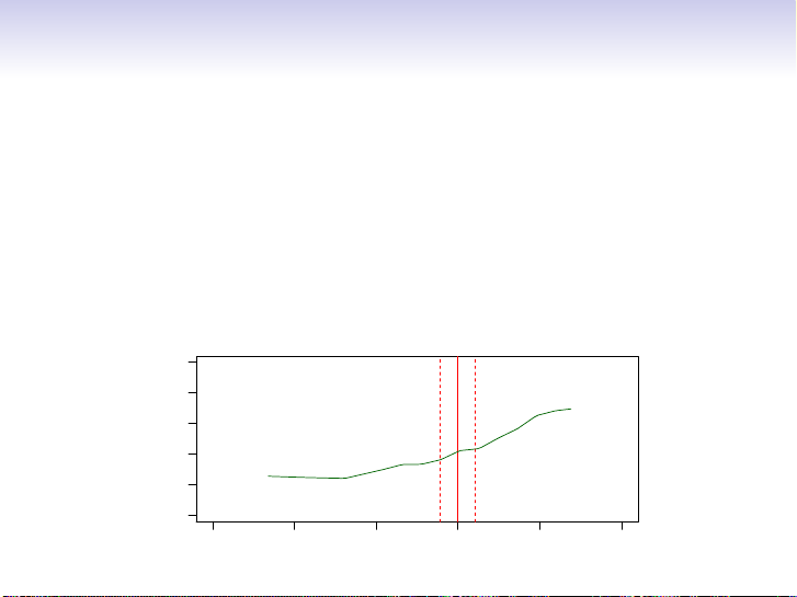
• Typically we have few if any data points with X = 4 exactly.
• So we cannot compute E(Y |X = x)!
• Relax the definition and let ˆ f (x) = Ave(Y |X ∈ N (x))
where N (x) is some neighborhood of x. 3 ● ● 2 ● ● ● ● ● ● ● ● ● ● ● ● 1 ● ● ● ● ● ● ● y ● ●● ● ● ● ● ● ● ● ● ● 0 ● ● ● ● ● ● ● ● ● ● ● ● ● ● ● ● ● ● ●● ● ● ● ● ● ● ● ● ● ● ● ● ● ● ● −1 ●● −2 1 2 3 4 5 6 x 6 / 30
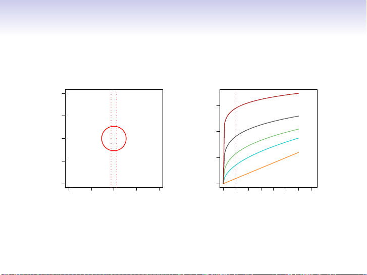
• Nearest neighbor methods can be lousy when p is large.
Reason: the curse of dimensionality. Nearest neighbors
tend to be far away in high dimensions.
• We need to get a reasonable fraction of the N values of yi
to average to bring the variance down—e.g. 10%.
• A 10% neighborhood in high dimensions need no longer be
local, so we lose the spirit of estimating E(Y |X = x) by local averaging.
• Nearest neighbor averaging can be pretty good for small p
— i.e. p ≤ 4 and large-ish N.
• We will discuss smoother versions, such as kernel and
spline smoothing later in the course. 7 / 30
• Nearest neighbor averaging can be pretty good for small p
— i.e. p ≤ 4 and large-ish N.
• We will discuss smoother versions, such as kernel and
spline smoothing later in the course.
• Nearest neighbor methods can be lousy when p is large.
Reason: the curse of dimensionality. Nearest neighbors
tend to be far away in high dimensions.
• We need to get a reasonable fraction of the N values of yi
to average to bring the variance down—e.g. 10%.
• A 10% neighborhood in high dimensions need no longer be
local, so we lose the spirit of estimating E(Y |X = x) by local averaging. 7 / 30 The curse of dimensionality 10% Neighborhood p= 10 ● 1.0 ● ● ●● ● ● ● ● ● ● ● ● ● ● ● ● ● ● ● ● ● 1.5 ● ● ● ● ● ● ● ● 0.5 p= 5 ● ● ● ● ● ● ● ● p= 3 ● ● ● ● 1.0 ● ● ● ● ● ● ● x2 p= 2 ● ● ● 0.0 ● ● ●● ● ● ● ● ● Radius ● ● ● ● ● ● p= 1 ● ● ● ● ● ● ● ● ● ● 0.5 ● ● ● ● ● −0.5 ●● ● ● ● ● ● ● ● ● ● ● ● ● ● ● ● ● ● −1.0 0.0 −1.0 −0.5 0.0 0.5 1.0 0.0 0.1 0.2 0.3 0.4 0.5 0.6 0.7 x1 Fraction of Volume 8 / 30
Parametric and structured models
The linear model is an important example of a parametric model:
fL(X) = β0 + β1X1 + β2X2 + . . . βpXp.
• A linear model is specified in terms of p + 1 parameters β0, β1, . . . , βp.
• We estimate the parameters by fitting the model to training data.
• Although it is almost never correct, a linear model often
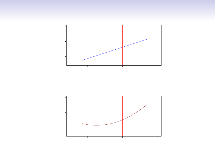
serves as a good and interpretable approximation to the unknown true function f (X). 9 / 30 A linear model ˆ fL(X) = ˆ β0 + ˆ
β1X gives a reasonable fit here 3 ● ● 2 ● ● ● ● ● ● ● ● ● ● ● ● 1 ● ● ●● ● ● ● ● y ● ● ● ● ● ● ● ● ● ● ● ● 0 ● ● ● ● ● ● ● ● ● ● ● ● ● ● ● ● ● ● ● ● ● ● ● ● ● ● ● ● ●● ● ● −1 ● ● ●● −2 1 2 3 4 5 6 x A quadratic model ˆ fQ(X) = ˆ β0 + ˆ β1X + ˆ β2X2 fits slightly better. 3 ● ● 2 ● ● ● ● ● ● ● ● ● ● ● ● 1 ● ● ●● ● ● ● ● y ● ● ● ● ● ● ● ● ● ● ● 0 ● ● ● ● ● ● ● ● ● ● ● ● ● ● ● ● ● ● ● ● ● ● ● ● ● ● ● ● ● ●● ● ● −1 ● ● ●● −2 1 2 3 4 5 6 x 10 / 30 Income ity Years of Education Senior
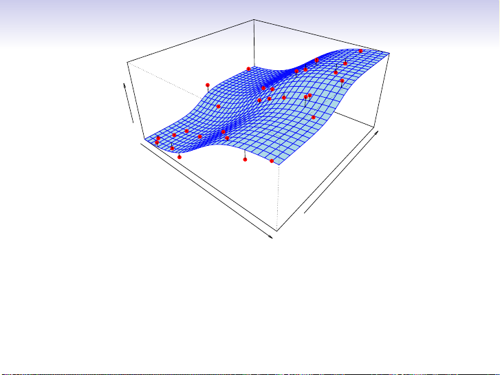
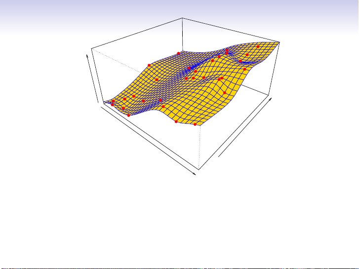
Simulated example. Red points are simulated values for income from the model
income = f (education, seniority) + f is the blue surface. 11 / 30 Income ity Years of Education Senior
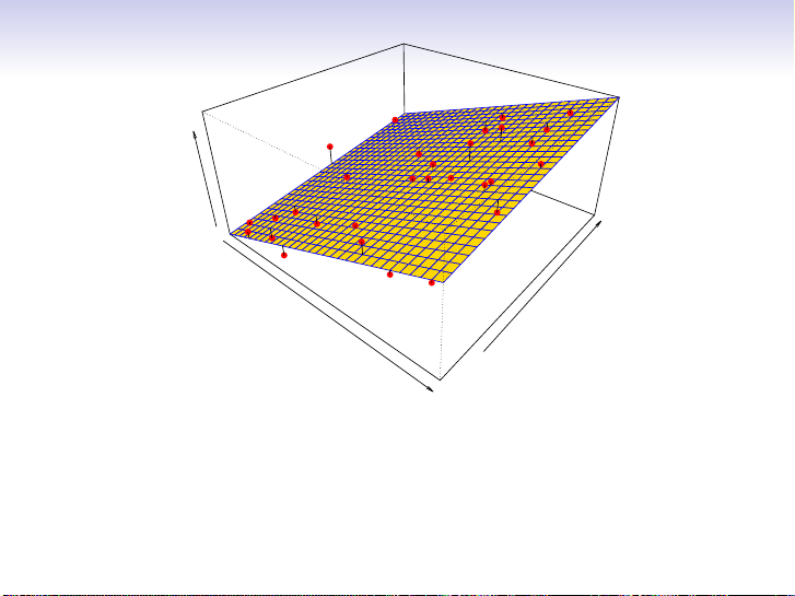
Linear regression model fit to the simulated data. ˆ fL(education, seniority) = ˆ β0+ ˆ β1×education+ ˆ β2×seniority 12 / 30 Income ity Years of Education Senior
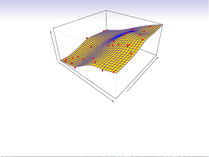
More flexible regression model ˆ
fS(education, seniority) fit to
the simulated data. Here we use a technique called a thin-plate
spline to fit a flexible surface. We control the roughness of the fit (chapter 7). 13 / 30 Income ity Years of Education Senior
Even more flexible spline regression model ˆ
fS(education, seniority) fit to the simulated data. Here the
fitted model makes no errors on the training data! Also known as overfitting. 14 / 30
• Good fit versus over-fit or under-fit.
— How do we know when the fit is just right?
• Parsimony versus black-box.
— We often prefer a simpler model involving fewer
variables over a black-box predictor involving them all. Some trade-offs
• Prediction accuracy versus interpretability.
— Linear models are easy to interpret; thin-plate splines are not. 15 / 30
• Parsimony versus black-box.
— We often prefer a simpler model involving fewer
variables over a black-box predictor involving them all. Some trade-offs
• Prediction accuracy versus interpretability.
— Linear models are easy to interpret; thin-plate splines are not.
• Good fit versus over-fit or under-fit.
— How do we know when the fit is just right? 15 / 30
Tài liệu liên quan:
-

Tổng hợp lý thuyết và bài tập về Biến cố và Xác suất - Môn Xác suất TH101
5 3 -

Bài tập tham khảo môn Xác suất thống kê | Đại học Bách Khoa Hà Nội
22 11 -

Bài tập tham khảo Xác suất thống kê | Đại học Bách Khoa Hà Nội
16 8 -

đề thi cuối kì môn xác suất thống kê
27 14 -

Đề thi cuối kì học kỳ 1 năm 2023 môn Xác suất thống kê | Đại học Bách Khoa Hà Nội
32 16