Chapter 5 Lecture Notes: DCF Valuation Analysis | Môn Investment Banking - Trường Đại học Quốc tế, Đại học Quốc gia Thành phố Hồ Chí Minh

lOMoAR cPSD| 58562220
Chapter 5: Valuation: Discounted Cash Flow (DCF) Analysis 1.Definition
• DCF analysis is a fundamental valuation methodology broadly used. It
is premised on the principle that the value of a company, division,
business, or collection of assets (“target”) can be derived from the
present value of its projected free cash flow (FCF).
• Intrinsic value can be derived from PV of projected free cash flow
• Important alternative to market-based valuation techniques
• Typically, FCF is projected for 5 years. Terminal value (“going
concern” value) captures remaining value beyond projection period
• WACC is the discount rate commensurate with business and financial risks
• Sensitivity analysis is used to test assumptions 2.
Steps Step 1: Study the target and determine key performance drivers Study the Target
• Study and learn as much as possible about the target and its sector. A
thorough understanding of the target’s business model, financial profile,
value proposition for customers, end markets, competitors, and key
risks is essential for developing a framework for valuation. Source of
info: SEC filings, earnings call transcripts, investor presentations,
MD&A section, equity research reports.
Determine key performance drivers (sales growth, profitability, FCF generation):
• Internal: new facilities/stores/products/customer contracts, improve
operational and working capital efficiency lOMoAR cPSD| 58562220
• External: acquisitions, end market trends, consumer buying patterns,
macroeconomic factors, legislative/regulatory changes.
Step 2: Project Free Cash Flow
Free Cash Flow: cash generated after paying all cash operating expenses and
taxes and after funding capex and working capital, but before paying interest expense.
FCF is independent of capital structure.
FCF = EBIT – Taxes + D&A – Capex – Increase (Decrease) in Net WC
= EBIT(1-Tc) + D&A – Capex – Increase (Decrease) in Net WC
Considerations for Projecting Free Cash Flow
• Historical performance: Historical performance provides valuable
insight for developing defensible assumptions to project. The DCF
customarily begins by laying out the target’s historical financial data for
the prior three-year period financial statements with adjustments for
non-recurring items and recent events
• Projection period length: 5 years, or when financial performance reaches steady stage
• Alternative cases: Management case, Base case, and upside and downside cases
Projection of Sales, EBITDA, and EBIT Sale Projection
• Using consensus estimates, equity research, industry reports, consulting
studies. Be aware of cyclical business
• Compare projections with target’s historical growth rates, peer
estimates, sector/market outlook
• Growth assumptions need to be justifiable
• Sales projections are consistent with other related assumptions (capex, working capital) lOMoAR cPSD| 58562220
COGS and SG&A Projections
• Historical gross profit margin and SG&A as a percentage of sales
• For private companies, examine research estimates for peer companies
EBITDA and EBIT Projection
• For future 2 or 3 years: use consensus estimates
• For outer years: hold margins constant at the last year level provided by
consensus estimates, consider profitability increasing or decreasing
• For private companies: use historical trends and consensus estimates for peer companies Tax Projection
• The first step in calculating FCF from EBIT is to subtract estimated
taxes. The result is tax-effected EBIT, also known as EBIAT or NOPAT.
This calculation involves multiplying EBIT by (1 – t), where “t” is the target’s marginal tax rate.
• A marginal tax rate of 35% to 40% is generally assumed for modeling purposes.
• The company’s actual tax rate (effective tax rate) in previous years can
also serve as a reference point D&A Projections
• Depreciation: projected as percentage of sales or capex based on
historical levels. Or build a detailed PP&E schedule. Ensure
depreciation and capex are in line by the final year of projection period
• Amortization: projected as percentage of sale, or build detailed
schedule based on existing intangible assets
• For some companies, D&A is a separate line item on income statement.
But more commonly included in COGS or SG&A. lOMoAR cPSD| 58562220
• D&A as one line-item: projected using 2 methods for depreciation
above, or D&A = EBITDA - EBIT
• D&A is non-cash expense. It is added back to EBIAT in the calculation
of FCF. Hence, while D&A decreases a company’s reported earnings, it does not decrease its FCF.
Capital expenditure Projection
• Historical capex is a reliable proxy
• Consider company’s strategy, sector, or phase of operations
• Future planned capex can be found in MD&A section, research reports
• Generally driven as percentage of sales in line with historical levels
Change in net working capital Projections
• An increase in NWC is a use of cash. A decrease in NWC is a source of cash
• NWC is projected as percentage of sales
• Recommended approach is to project each component of current assets
and current liabilities which is projected based on historical ratios from
prior year level or 3-year average
Change in NWC = NWC in year n – NWC in year (n-1)
NWC = Non-cash current assets – Non-interest-bearing current liabilities
= (A/R + Inventory + Prepaid expenses and Other current assets) – (A/P
+ Accrued liabilities + Other current liabilities)
• Accounts receivable: use DSO
• Inventory: use DIH or Inventory turns
• Prepaid expenses and Other current assets: projected as percentage of
sales in line with historical levels lOMoAR cPSD| 58562220 • Accounts payable: use DPO
• Accrued liabilities and Other current liabilities: projected as percentage
of sales in line with historical levels
DSO (Day sale outstanding) = (A/R / Sales)*365
DIH (Days inventory held) = (Inventory/COGS)*365 Inventory Turns =
COGS/Inventory DPO = (A/P / COGS) * 365 Step 3: Calculate
Weighted Average Cost of Capital
WACC is also called opportunity cost of capital Steps for calculating WACC:
• Determine target capital structure
• Estimate cost of debt (rd)
• Estimate cost of equity (re)
Calculate WACC : rWACC = rd* (1-T) * D/(D+E) + re * E/(E+D)
Often use WACC range by sensitizing its key inputs
Target capital structure: is consistent with long-term strategy. Use company’s
current and historical debt-to-total capitalization ratios, or mean and median
of its peers. Target capital structure is held constant throughout projection period.
Cost of debt (rd): if company is currently at its target capital structure, , cost
of debt is derived from blended yield on outstanding debt instruments
(public and private debt). Otherwise, cost of debt is derived from peer companies
• Publicly traded bonds: current yield on all outstanding issues
• Private debt (revolving credit facilities and term loans): consults with
debt capital markets specialist for current yield lOMoAR cPSD| 58562220
• If no current market data, use at-issuance coupons of current debt
maturities, or estimate company’s credit rating at target capital structure
and use cost of debt for comparable credits
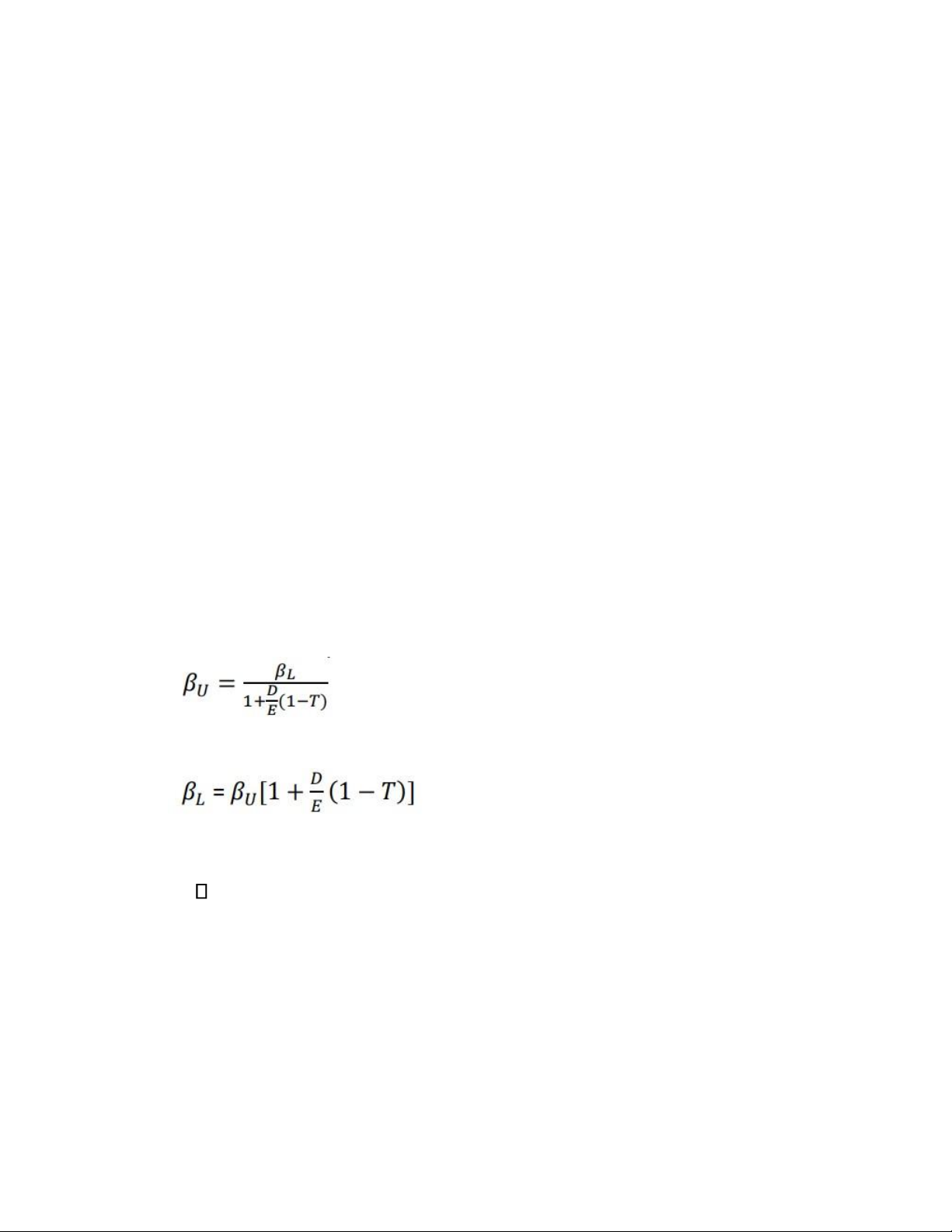
Cost of equity (re): use CAPM
• Cost of equity = Risk-free rate + Levered beta x Market risk premium
• Beta for public company: use historical beta
• Beta for private company: is derived from a group of publicly traded
peer companies, but need to neutralize the effects of different capital structures:
✓ Calculate unlevered beta (asset beta) of each peer, then take the average
✓ Calculate relevered beta using company’s target capital structure and marginal tax rate
How to calculate levered beta for private company:
Unlevered beta (asset beta) of each peer:
Relevered beta of the target company:
Note: Use avarege 𝛽𝑈 to calculate
Size premium (SP): added to cost of equity of CAPM
re = rf + 𝛽L * (rm –rf) + SP lOMoAR cPSD| 58562220
Step 4: Determine Terminal Value
Terminal value is typically calculated on the basis of the company’s FCF (or
a proxy such as EBITDA) in the final year of the projection period.
Exit multiple method (EMM):
Terminal value = EBITDAn x Exit Multiple
n: terminal year of projection period. Multiple is the current LTM trading
multiples for comparable companies
Use normalized trading multiple, normalized EBITDA
Sensitivity analysis: range of exit multiple Perpetuity growth method (PGM):
Terminal value = [FCFn x (1+g)] / (r-g)
FCF: unlevered free cash flow n: terminal
year of projection period FCF: unlevered free
cash flow g: perpetuity growth rate (2% to 4%) r: WACC
Perpetuity growth rate:
• Based on company’s expected long-term industry growth rate (2%-4%)
• Is sensitized to produce valuation range
The followings are calculated to check between EMM and PGM: lOMoAR cPSD| 58562220
Implied perpetuity growth rate (end-of-year discounting and mid-year
discounting) Implied exit multiple (end-of-year discounting and mid-
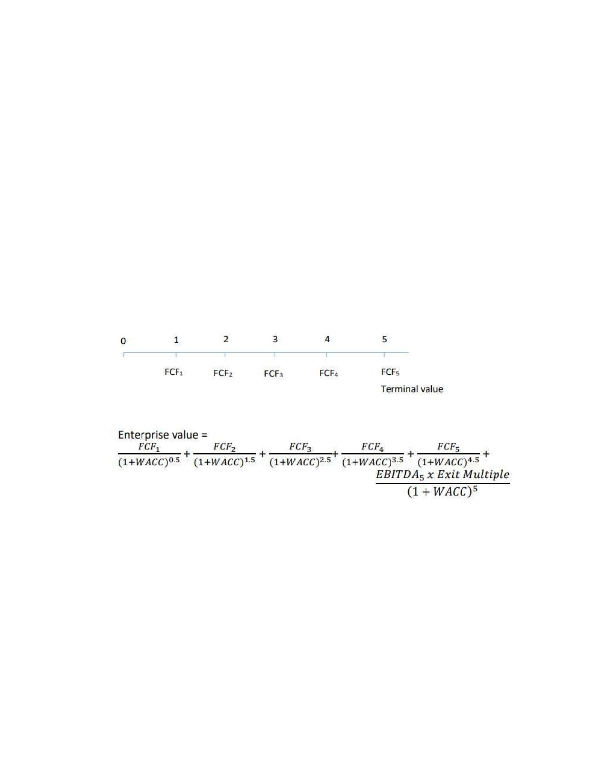
year discounting) Step 5: Calculate Present Value and Determine Valuation
Discount factor: year-end and mid-year convention
• Year end: Discount factor = 1/(1+WACC)n
• Mid year: Discount factor = 1/(1+WACC)n-0.5
Terminal value considerations: if using mid-year convention for FCF of
projection period, use mid-year discounting for terminal value under PGM,
but use year-end discounting under EMM Enterprise value
Using mid-year discounting with EMM method:
Implied equity value = Enterprise Value + Prefrerred Stock + Noncontrolling Interest
Implied share price = Implied equity value/Fully Diluted Shares Outstanding
• Sensitivity analysis: The exercise of deriving a valuation range by
varying key inputs is called sensitivity analysis. Key valuation drivers
such as WACC, exit multiple, and perpetuity growth rate are the most
commonly sensitized inputs in a DCF lOMoAR cPSD| 58562220 Key Pros
• Cash flow-based: reflects value of projected FCF, a more fundamental approach to valuation
• Market independent: more insulated from market bubbles and distressed periods
• Self-sufficient: DCF is important when there are limited or no “pure play” public comparables
• Flexibility: can run multiple financial performance scenarios (growth
rates, margins, capex requirements, working capital efficiency) Key cons
• Dependence on financial projections: accurate forecasting of financial
performance is challenging, especially as projection period lengthens
• Sensitivity to assumptions: small changes in key assumptions (growth
rates, margins, WACC, exit multiple) can produce different valuation ranges
• Terminal value: accounts for three-quarters or more of DCF valuation
=> decrease the relevance of FCF of projection period
• Assumes constant capital structure: no flexibility to change capital
structure over projection period
1.Calculate FCF using the information below Assumptions EBIT $300 D&A 50 Capex 25
Inc/(Dec) in Net Working Capital 10 Tax Rate 38% lOMoAR cPSD| 58562220
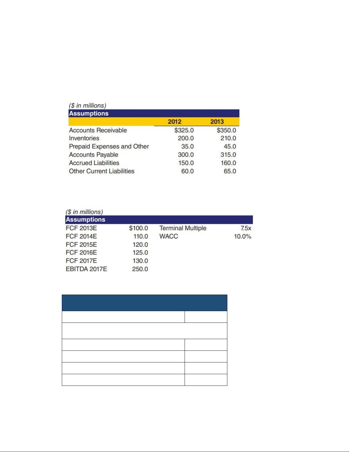
2. Calculate the (increase) / decrease in net working capital from 2012 to 2013
based on the following assumptions
3. Using a mid-year convention and the assumptions below,calculate enterprise value
4. Using the information below to answer question Enterprise Value Cumulative PV of FCF $1,600 Terminal Value Terminal year EBITDA $929.2 Exit Multiple 7.5x Terminal Value Discount Factor 0.62 lOMoAR cPSD| 58562220 PV of Terminal Value % of Enterprise Value Enterprise Value a) Calculate Terminal Value b) Calculate Enterprise Value
c) Calculate the percentage of enterprise value represented by the terminal value