Determinants of the Balance of Trade - Elasticities & Absorption | Tài chính quốc tế | Trường Học Viện nông nghiệp Việt Nam
Earlier chapters are full of discussions involving foreign exchange rates and the balance of payments. We now know the definitions and uses of these two important international finance terms, but have yet to consider what determines their values at any particular point in time.Why do some countries run a balance of trade surplus while others run deficits? It is worth noting that financial institutions, central banks, and governments invest many resources in trying to predict exchange rates and international trade and payments. Tài liệu được sưu tầm và soạn thảo dưới dạng file PDF để gửi tới các bạn cùng tham khảo, ôn tập đầy đủ kiến thức, chuẩn bị cho các buổi học thật tốt. Mời bạn đọc đón xem!
Môn: Tài chính quốc tế (hvnn) 130 tài liệu
Trường: Học viện Nông nghiệp Việt Nam 2.4 K tài liệu
Tác giả:

Preview text:
CHAPTER 12
Determinants of the Balance of Trade Contents
Elasticities Approach to the Balance of Trade 233 Elasticities and the J-Curve 238 Currency Contract Period 238 Pass-Through Analysis 240
The Marshall–Lerner Condition 244
The Evidence From Devaluations 246
Absorption Approach to the Balance of Trade 247 Summary 249 Exercises 250 Further Reading 250
Earlier chapters are full of discussions involving foreign exchange rates
and the balance of payments. We now know the definitions and uses of
these two important international finance terms, but have yet to consider
what determines their values at any particular point in time. Why do some
countries run a balance of trade surplus while others run deficits? It is
worth noting that financial institutions, central banks, and governments
invest many resources in trying to predict exchange rates and international
trade and payments. The kinds of theories to be introduced in this chap-
ter have shaped the way economists, investors, and politicians approach
such problems. Exchange rate determination will be discussed in the next chapters.
ELASTICITIES APPROACH TO THE BALANCE OF TRADE
Economic behavior involves satisfying unlimited wants with limited
resources. One implication of this fact of budget constraints is that con-
sumers and business firms will substitute among goods as prices change to
stretch their budgets as far as possible. For instance, if Italian-made shoes
and US-made shoes are good substitutes, then as the price of US shoes © 201 7 Elsevier Inc.
International Money and Finance. All rights reserved. 233 234
International Money and Finance
rises relative to Italian shoes, buyers will substitute the lower-priced Italian
shoes for the higher-priced US shoes. The crucial concept for determining
consumption patterns is relative price—the price of one good relative to
another. Relative prices change as relative demand and supply for individual
goods change. Such changes may result from changes in tastes, or produc-
tion technology, or government taxes or subsidies, or many other possible
sources. If the changes involve prices of goods at home changing relative to
foreign goods, then international trade patterns may be altered. The elastici-
ties approach to the balance of trade is concerned with how changing rela-
tive prices of domestic and foreign goods will change the balance of trade.
A change in the exchange rate will change the domestic currency price
of foreign goods. Suppose initially that a pair of shoes sells for $50 in the
United States and €50 in Italy. At an exchange rate of €1 = $1, the shoes
sell for the same price in each country when expressed in a common cur-
rency. If the euro is devalued to €1.2 = $1, and shoe prices remain con-
stant in the domestic currency of the producer, then shoes selling for €50
in Italy will now cost the US buyer $41.67. After the devaluation, €1 =
$0.8333, so €50 = $41.67, and the price of Italian shoes has fallen for US
buyers. Conversely, the price of $50 US shoes to Italian buyers has risen
from €50 to €60. The relative price effect of the euro devaluation should
increase US demand for Italian goods and decrease Italian demand for US
goods. How much quantity demanded changes in response to the relative
price change is determined by the elasticity of demand.
In the beginning of economics courses, students learn that elasticity
measures the responsiveness of quantity to changes in price. The elastici-
ties approach to the balance of trade provides an analysis of how devaluations
will affect the balance of trade depending on the elasticities of supply and
demand for foreign exchange and foreign goods.
When demand or supply is elastic, it means that quantity demanded or
supplied will be relatively responsive to the change in price. An inelastic
demand or supply indicates that quantity is relatively unresponsive to price
changes. We can make things more precise by using coefficients of elastic-
ity. For instance, letting ε represent the coefficient of elasticity of demand, d we can write ε as d ε = %∆Q/%∆P d (12.1)
This implies that the coefficient of elasticity of demand is equal to the per-
centage change in the quantity demanded, divided by the percentage change
in price. If the price increases by 5% and the quantity demanded falls by more
Determinants of the Balance of Trade 235
than 5%, then εd exceeds 1 (in absolute value), and we say that demand is elas-
tic. If the price increases by 5%, but quantity demanded falls by less than 5%,
we would say that demand is inelastic and εd would be less than 1.
Just as we can compute a coefficient of elasticity of demand ε , so too d
can we compute a coefficient of elasticity of supply, ε , as the percent- s
age change in the quantity supplied, divided by the percentage change in
price. If ε exceeds 1, the quantity supplied is relatively responsive to price, s
and we say that supply is elastic. For ε less than 1, the quantity supplied is s
relatively unresponsive to price, so that the supply is inelastic.
Elasticity will determine what happens to total revenue (sales price
times quantities sold) following a price change. For example, an elastic
demand is when quantity changes exceed that of the price change. In such
a case, the total revenue will move in the opposite direction from the price
change. Suppose the demand for black velvet paintings from Mexico is
elastic. If the peso price rises 10%, the quantity demanded falls by more
than 10%, so that the revenue received from sales will fall as a result of the
price change. In contrast, if the demand for Colombian coffee is inelastic,
then a 10% increase in price will result in a fall in the quantity demanded
of less than 10%. The high coffee price increase more than makes up for
the lost sales. Thus, coffee sales revenues rise following the price change.
Obviously, the elasticity of demand is very important in determining
export and import revenues when international prices change.
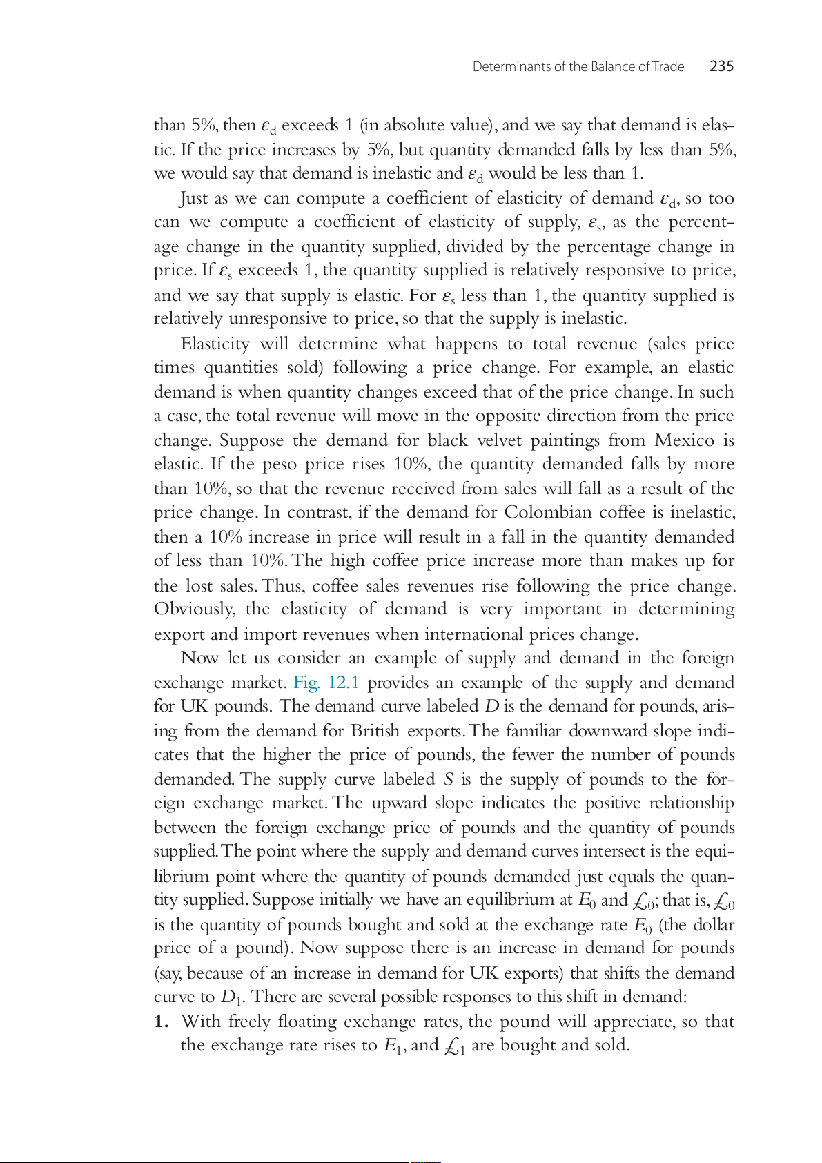
Now let us consider an example of supply and demand in the foreign
exchange market. Fig. 12.1 provides an example of the supply and demand
for UK pounds. The demand curve labeled D is the demand for pounds, aris-
ing from the demand for British exports. The familiar downward slope indi-
cates that the higher the price of pounds, the fewer the number of pounds
demanded. The supply curve labeled S is the supply of pounds to the for-
eign exchange market. The upward slope indicates the positive relationship
between the foreign exchange price of pounds and the quantity of pounds
supplied. The point where the supply and demand curves intersect is the equi-
librium point where the quantity of pounds demanded just equals the quan-
tity supplied. Suppose initially we have an equilibrium at E0 and £ ; that is, £ 0 0
is the quantity of pounds bought and sold at the exchange rate E0 (the dollar
price of a pound). Now suppose there is an increase in demand for pounds
(say, because of an increase in demand for UK exports) that shifts the demand
curve to D1. There are several possible responses to this shift in demand:
1. With freely floating exchange rates, the pound will appreciate, so that
the exchange rate rises to E , and £ are bought and sold. 1 1 236
International Money and Finance E S E1 E0 D1 D0 0 £ ' 0 £1 £ £ 1
Figure 12.1 Supply and demand in the foreign exchange market.
2. Central banks can peg the exchange rate at the old rate E by provid- 0
ing £ ′ − £ from their reserves. 1 0
3. The supply and demand can be affected by imposing controls or quo-
tas on the supply of, or demand for, pounds.
4. Quotas or tariffs could be imposed on foreign trade to maintain the
old supply and demand for pounds.
The elasticities approach recognizes that the effect of an exchange rate
change on the equilibrium quantity of currency being traded will depend
on the elasticities of the supply and demand curves involved. It is impor-
tant to remember that the elasticities approach is a theory of the balance
of trade and can only be a theory of the balance of payments in a world without capital flows.
Suppose that in Fig. 12.1, the US central bank (the Federal Reserve)
decides to fix the exchange rate at E . To do so the US central bank has to 0
supply pounds to the market from US reserves in exchange for US dol-
lars. Now the old exchange rate E is maintained because of the central 0
bank’s addition of £ ′ − £ to the market. If it becomes apparent that the 1 0
increase in demand is a permanent change, then the Federal Reserve will
have to devalue the dollar, driving up the dollar price of pounds. This, of
course, means that UK goods will be more expensive to the United States,
whereas US goods will be cheaper to the United Kingdom. Will this
improve the US trade balance? It all depends on the elasticities of supply
and demand. When the quantity demanded for the imports by American
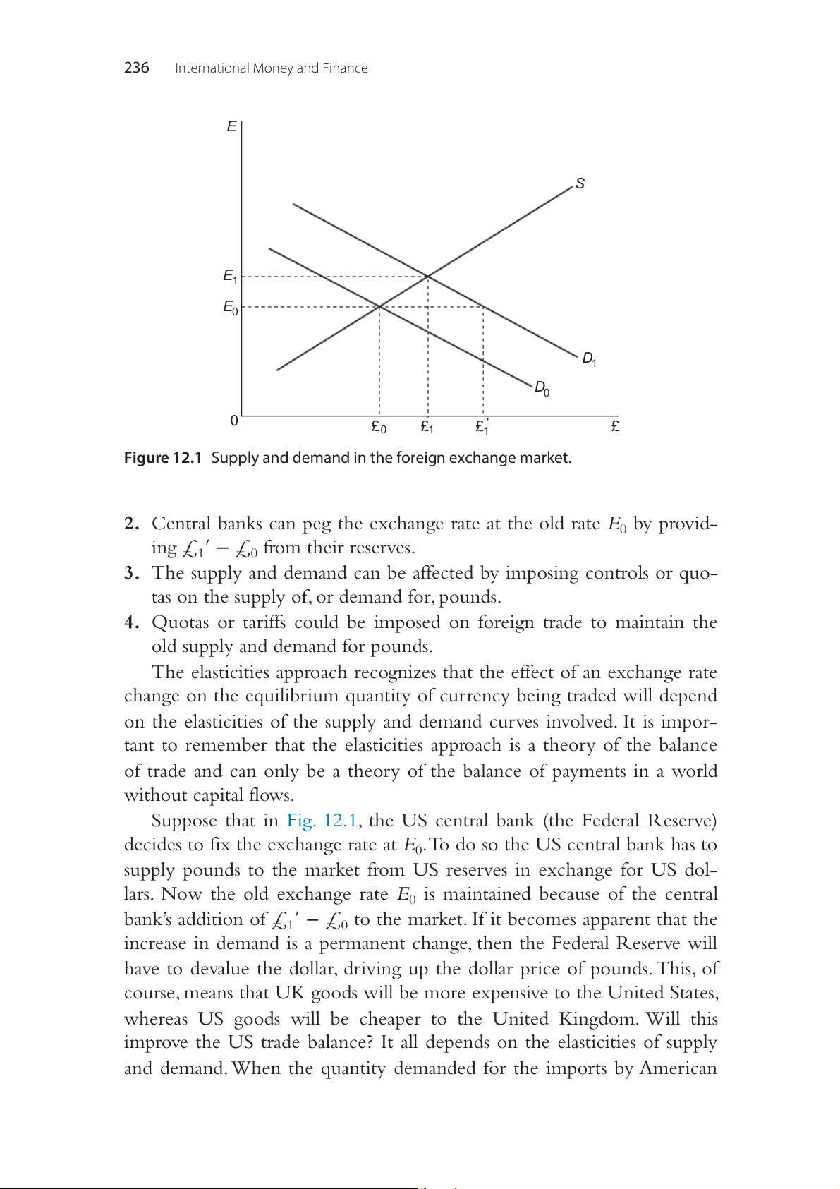
Determinants of the Balance of Trade 237 e d f tra o 0 Time ce t n 0 la a B
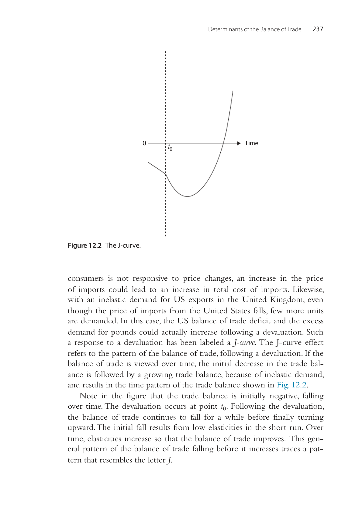
Figure 12.2 The J-curve.
consumers is not responsive to price changes, an increase in the price
of imports could lead to an increase in total cost of imports. Likewise,
with an inelastic demand for US exports in the United Kingdom, even
though the price of imports from the United States falls, few more units
are demanded. In this case, the US balance of trade deficit and the excess
demand for pounds could actually increase following a devaluation. Such
a response to a devaluation has been labeled a J-curve. The J-curve effect
refers to the pattern of the balance of trade, following a devaluation. If the
balance of trade is viewed over time, the initial decrease in the trade bal-
ance is followed by a growing trade balance, because of inelastic demand,
and results in the time pattern of the trade balance shown in Fig. 12.2.
Note in the figure that the trade balance is initially negative, falling
over time. The devaluation occurs at point t . Following the devaluation, 0
the balance of trade continues to fall for a while before finally turning
upward. The initial fall results from low elasticities in the short run. Over
time, elasticities increase so that the balance of trade improves. This gen-
eral pattern of the balance of trade falling before it increases traces a pat-
tern that resembles the letter J. 238
International Money and Finance
ELASTICITIES AND THE J-CURVE
Devaluation is conventionally believed to be a tool for increasing a coun-
try’s balance of trade. Yet the J-curve effect indicates that when devaluation
increases the price of foreign goods to the home country and decreases
the price of domestic goods to foreign buyers, there is a short-run period
during which the balance of trade falls. We now consider the reasons for
why there may be low elasticities in the short run, to see what the possible
underlying reasons are for a J-curve. We can identify two different periods
following a devaluation. Immediately following a devaluation the contracts
that have already been negotiated become revalued. Such a period is called
the currency contract period. Once the contracts have expired there may still
be a limited response by traders. The short-run period following the expi-
ration of contracts is called the pass-through analysis. During this period the
traders have limited changes in the quantities in response to the new set of
prices, but over time the response becomes complete. We will discuss each
of these two short-run responses.
CURRENCY CONTRACT PERIOD
Immediately following a devaluation, contracts negotiated prior to the
exchange rate change become due. This period is called the currency contract
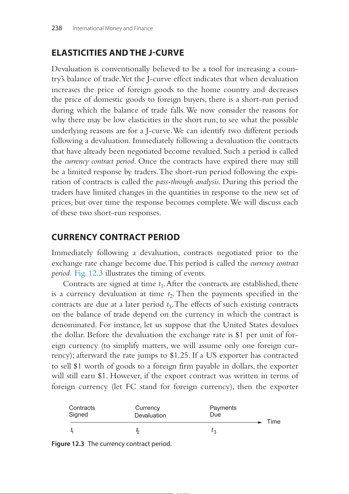
period. Fig. 12.3 illustrates the timing of events.
Contracts are signed at time t . After the contracts are established, there 1
is a currency devaluation at time t . Then the payments specified in the 2
contracts are due at a later period t . The effects of such existing contracts 3
on the balance of trade depend on the currency in which the contract is
denominated. For instance, let us suppose that the United States devalues
the dollar. Before the devaluation the exchange rate is $1 per unit of for-
eign currency (to simplify matters, we will assume only one foreign cur-
rency); afterward the rate jumps to $1.25. If a US exporter has contracted
to sell $1 worth of goods to a foreign firm payable in dollars, the exporter
will still earn $1. However, if the export contract was written in terms of
foreign currency (let FC stand for foreign currency), then the exporter Contracts Currency Payments Signed Devaluation Due Time t t t 1 2 3
Figure 12.3 The currency contract period.
Determinants of the Balance of Trade 239
expected to receive FC1, which would be equal to $1. Instead, the devalu-
ation leads to FC1 = $1.25, so the US exporter receives an unexpected
gain from the dollar devaluation. On the other hand, consider an import
contract where a US importer contracts to buy from a foreign firm. If the
contract calls for payment of $1, then the US importer is unaffected by
the devaluation. If the contract had been written in terms of foreign cur-
rency so that the US importer owes FC1, then the importer would have
to pay $1.25 to buy the FC1 that the exporter receives. In this case the
importer faces a loss because of the devaluation.
In the simple world under consideration here, we would expect sellers
to prefer a contract in the currency expected to appreciate, whereas buy-
ers would prefer contracts written in terms of the currency expected to
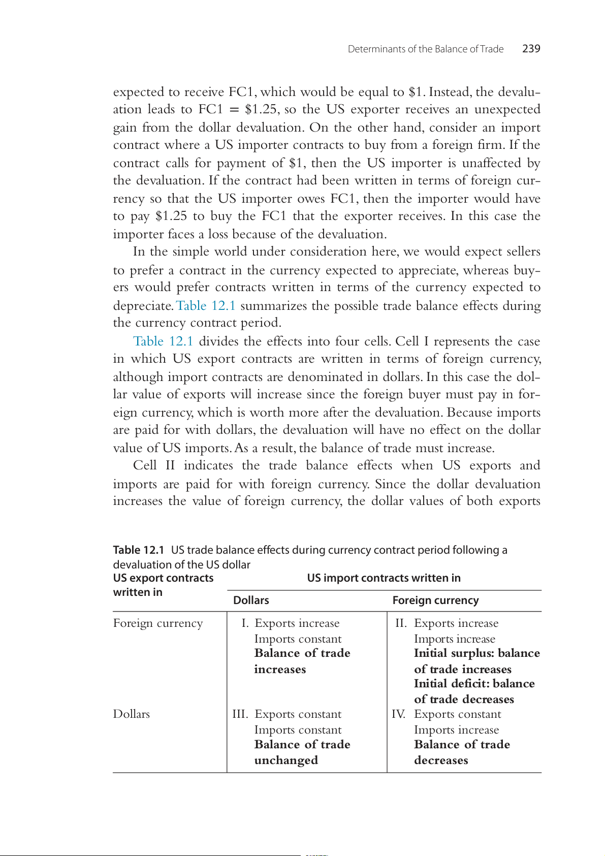
depreciate. Table 12.1 summarizes the possible trade balance effects during the currency contract period.
Table 12.1 divides the effects into four cells. Cell I represents the case
in which US export contracts are written in terms of foreign currency,
although import contracts are denominated in dollars. In this case the dol-
lar value of exports will increase since the foreign buyer must pay in for-
eign currency, which is worth more after the devaluation. Because imports
are paid for with dollars, the devaluation will have no effect on the dollar
value of US imports. As a result, the balance of trade must increase.
Cell II indicates the trade balance effects when US exports and
imports are paid for with foreign currency. Since the dollar devaluation
increases the value of foreign currency, the dollar values of both exports
Table 12.1 US trade balance effects during currency contract period following a devaluation of the US dollar US export contracts
US import contracts written in written in Dollars Foreign currency Foreign currency I. Exports increase II. Exports increase Imports constant Imports increase Balance of trade
Initial surplus: balance increases of trade increases Initial deficit: balance of trade decreases Dollars III. Exports constant IV. Exports constant Imports constant Imports increase Balance of trade Balance of trade unchanged decreases 240
International Money and Finance
and imports will increase. The net effect on the US trade balance depends
on the magnitude of US exports relative to imports. If exports exceed
imports, so that there is an initial trade surplus, then the increase in export
values will exceed the increase in imports and the balance of trade will
increase. Conversely, if there is an initial trade deficit, so that imports
exceed exports, then the increase in imports will exceed the increase in
exports and the balance of trade will decrease.
If both exports and imports are payable in dollars, then the balance of
trade is unaffected by a devaluation, as indicated in Cell III. But if exports
are payable in dollars and imports require payment in foreign currency,
the dollar value of exports will be unaffected by the devaluation and
import values will increase; in this case the trade balance decreases as in
Cell IV. Note that only in the case of Cell IV is there a decline in the
trade balance during the currency contract period following a devalua-
tion. A decline could also occur in Cell II, although only if there is an
initial trade deficit. The key feature of Table 12.1 is that foreign-currency-
denominated imports provide a necessary condition for the US trade bal-
ance to take the plunge observed in the J-curve phenomenon during the currency contract period. PASS-THROUGH ANALYSIS
The currency contract period refers to the period following a devaluation
when contracts negotiated prior to the devaluation come due. During this
time it is assumed that goods prices do not adjust instantaneously to the
change in currency values. Eventually, of course, as new trade contracts
are negotiated, goods prices will tend toward the new equilibrium. Pass-
through analysis considers the ability of prices to adjust in the short run.
The kind of adjustment expected is an increase in the price of imported
goods in the devaluing country and a decrease in the price of this coun-
try’s exports to the rest of the world. If goods prices do not adjust in this
manner, then spending patterns will not be altered, so that the desirable
balance of trade effects of devaluation do not appear.
Devaluation is normally a response to a persistent and growing bal-
ance of trade deficit. As import prices rise in the devaluing country,
fewer imports should be demanded. At the same time, the lower price of
domestic exports to foreigners should increase the quantity demanded
for exported goods. The combination of a higher demand for domestic
exports and a lower domestic demand for imports should bring about
Determinants of the Balance of Trade 241
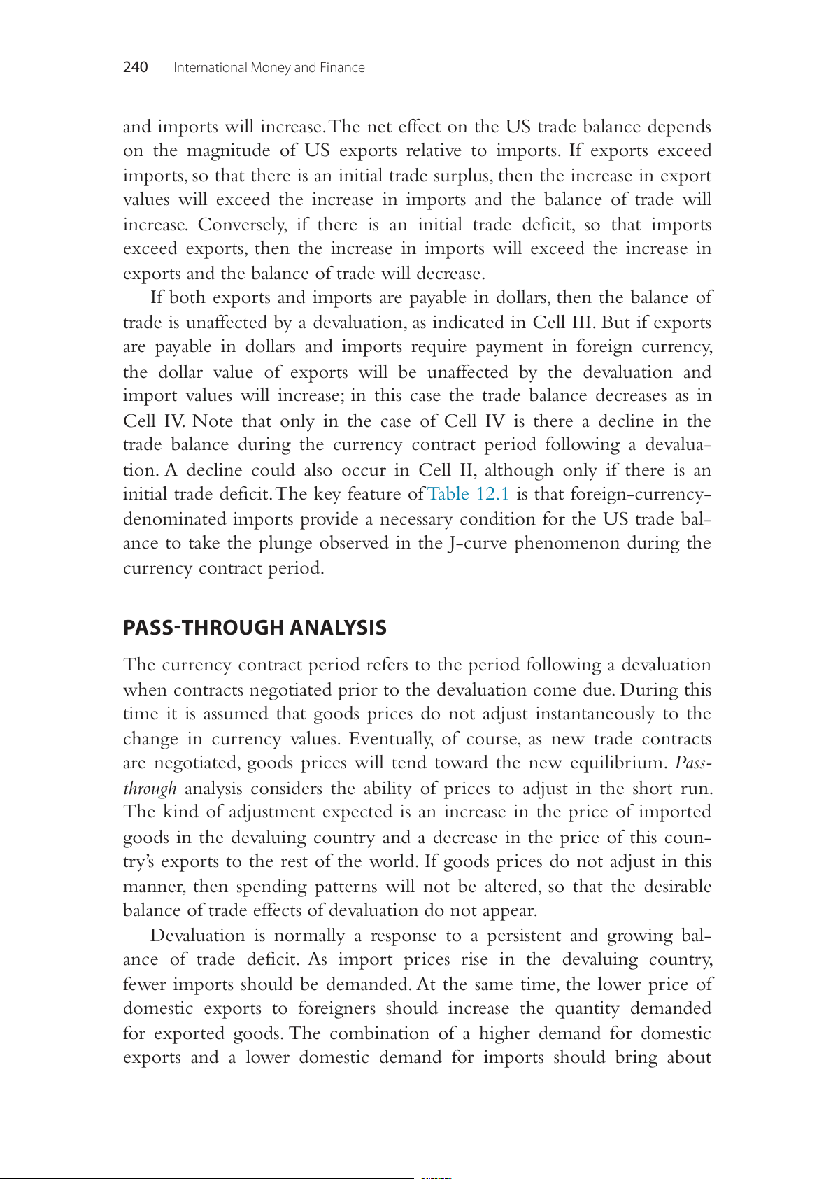
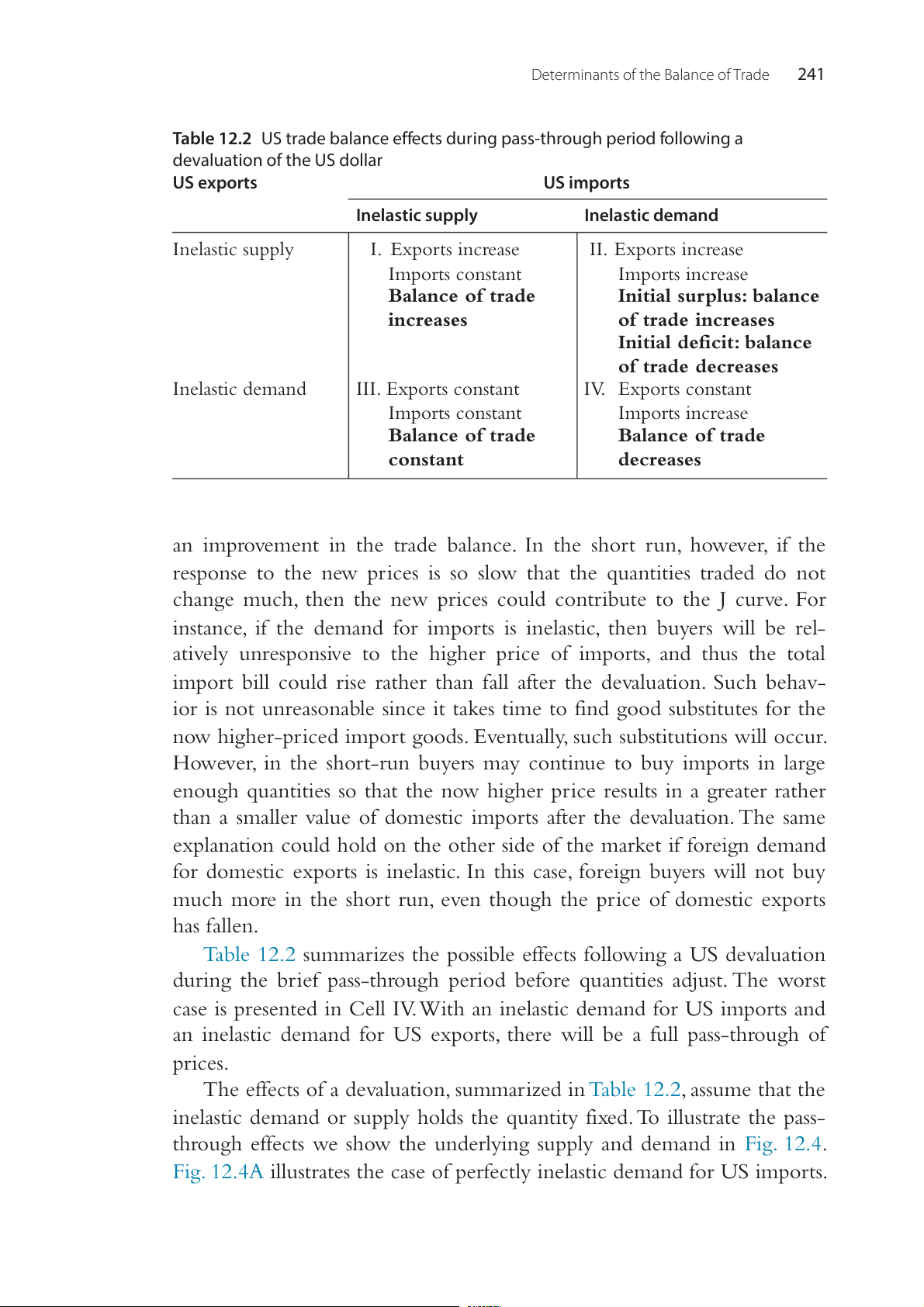
Table 12.2 US trade balance effects during pass-through period following a devaluation of the US dollar US exports US imports Inelastic supply Inelastic demand Inelastic supply I. Exports increase II. Exports increase Imports constant Imports increase Balance of trade
Initial surplus: balance increases of trade increases Initial deficit: balance of trade decreases Inelastic demand III. Exports constant IV. Exports constant Imports constant Imports increase Balance of trade Balance of trade constant decreases
an improvement in the trade balance. In the short run, however, if the
response to the new prices is so slow that the quantities traded do not
change much, then the new prices could contribute to the J curve. For
instance, if the demand for imports is inelastic, then buyers will be rel-
atively unresponsive to the higher price of imports, and thus the total
import bill could rise rather than fall after the devaluation. Such behav-
ior is not unreasonable since it takes time to find good substitutes for the
now higher-priced import goods. Eventually, such substitutions will occur.
However, in the short-run buyers may continue to buy imports in large
enough quantities so that the now higher price results in a greater rather
than a smaller value of domestic imports after the devaluation. The same
explanation could hold on the other side of the market if foreign demand
for domestic exports is inelastic. In this case, foreign buyers will not buy
much more in the short run, even though the price of domestic exports has fallen.
Table 12.2 summarizes the possible effects following a US devaluation
during the brief pass-through period before quantities adjust. The worst
case is presented in Cell IV. With an inelastic demand for US imports and
an inelastic demand for US exports, there will be a full pass-through of prices.
The effects of a devaluation, summarized in Table 12.2, assume that the
inelastic demand or supply holds the quantity fixed. To illustrate the pass-
through effects we show the underlying supply and demand in Fig. 12.4.
Fig. 12.4A illustrates the case of perfectly inelastic demand for US imports. 242
International Money and Finance Demand Demand rts o Supply (before) p Supply (after) cy n rts o f im rre xp Supply (after) o Supply (before) cu n f e rice ig o r p re o rice lla p o F D 0 Q0 0 QF Quantity of imports Quantity of exports (A) (B) Supply Supply rts o cy n rts xp o rre p f e o cu n f im o rice ig re r p o rice p Demand (before) F lla Demand (after) o Demand (after) D Demand (before) 0 QF 0 Q0 Quantity of imports Quantity of exports (C) (D)
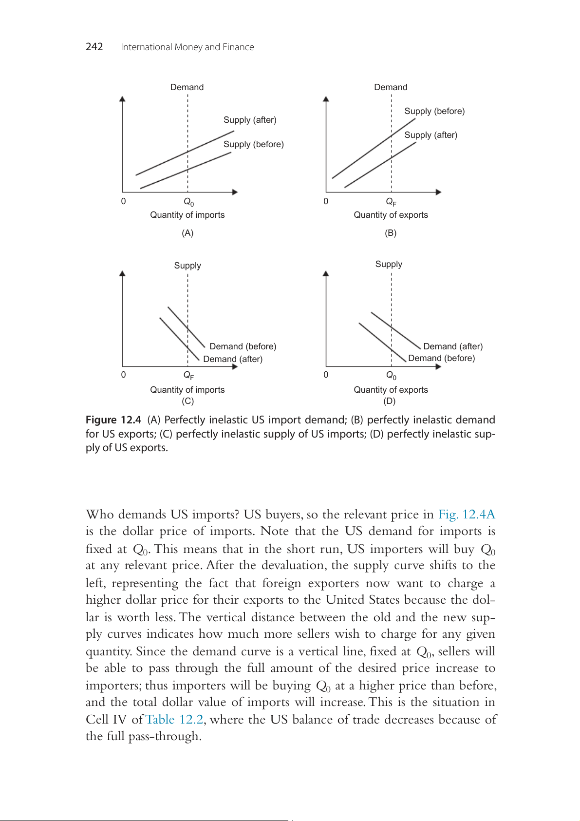
Figure 12.4 (A) Perfectly inelastic US import demand; (B) perfectly inelastic demand
for US exports; (C) perfectly inelastic supply of US imports; (D) perfectly inelastic sup- ply of US exports.
Who demands US imports? US buyers, so the relevant price in Fig. 12.4A
is the dollar price of imports. Note that the US demand for imports is
fixed at Q . This means that in the short run, US importers will buy 0 Q0
at any relevant price. After the devaluation, the supply curve shifts to the
left, representing the fact that foreign exporters now want to charge a
higher dollar price for their exports to the United States because the dol-
lar is worth less. The vertical distance between the old and the new sup-
ply curves indicates how much more sellers wish to charge for any given
quantity. Since the demand curve is a vertical line, fixed at Q , sellers will 0
be able to pass through the full amount of the desired price increase to
importers; thus importers will be buying Q at a higher price than before, 0
and the total dollar value of imports will increase. This is the situation in
Cell IV of Table 12.2, where the US balance of trade decreases because of the full pass-through.
Determinants of the Balance of Trade 243
Fig. 12.4B shows why exports remain constant in Cell IV. In this case
the foreigners’ demand for US exports is perfectly inelastic. Because for-
eign buyers purchase US exports, the relevant price is the foreign cur-
rency price in Fig. 12.4B. Foreign buyers want to purchase Q amount F
of US exports regardless of the price in the short run. Note that now the
relevant price to foreign buyers is the foreign currency price. After the
devaluation, the supply curve shifts to the right to reflect the fact that US
exporters are willing to sell goods for less foreign currency because for-
eign currency is now worth more. However, with the perfectly inelastic
demand curve, there is a full pass-through, lowering the foreign currency
price by the full amount of the devaluation. In other words, if the devalu-
ation increased the value of foreign currency by 10%, the foreign currency
price of US exports falls by 10% and the total dollar value of US exports remains constant.
Note that Cell III of Table 12.2 pairs the inelastic demand for US
exports, as just discussed, with an inelastic supply of US imports. Fig.
12.4C illustrates the effect of the inelastic supply. Since imports into the
United States are supplied by foreign sellers, the relevant price is the for-
eign currency price in Fig. 12.4C. In this case, foreign sellers will sell QF
imports to the United States independent of price. After the devalua-
tion, the US demand for imports in terms of foreign currency shifts to
the left, indicating that buyers are willing to pay fewer units of foreign
currency than before for a given quantity of imports. Because the sup-
ply curve is perfectly inelastic, the foreign currency price of imports falls
by the amount of the devaluation, and thus there is no pass-through. In
other words, the pass-through effect is completely offset by a fall in the
foreign currency price of imports. After a dollar devaluation we expect
imports to become more expensive to the United States; yet with a per-
fectly inelastic import supply curve, as in Fig. 12.4C, US dollar import
prices are unchanged so that the dollar value of imports is also unchanged.
Cell II of Table 12.2 couples the inelastic US import demand, as pre-
viously discussed and illustrated in Fig. 12.4A, with an inelastic supply of
US exports. Fig. 12.4D shows the supply effect. Because US exports are
supplied by US sellers, the dollar price is the relevant price in Fig. 12.4D.
After the devaluation, foreigners are willing to pay a higher dollar price
for US exports because dollars are cheaper. With the perfectly inelastic
supply curve, the dollar price of exports rises by the full amount of the
devaluation. Thus, rather than having a devaluation pass-through lower
US export prices to foreigners, the increase in dollar prices has foreign 244
International Money and Finance
buyers paying the same price as before (because the foreign currency price
is unchanged). But the higher dollar price results in an increase in the dol-
lar value of US exports. Since the inelastic demand for US imports also
causes the dollar value of imports to increase, the net result for the balance
of trade depends on whether initially exports exceeded imports, in which
case the increase in exports after the devaluation will be larger than the
import increase. If imports initially exceeded exports, then the devaluation will lower the trade balance.
Finally, we have the case of Cell I, where the balance of trade clearly
increases during the pass-through period when quantities are fixed. The
inelastic supply of US exports leads to an increase in the dollar value of
US exports, whereas the inelastic supply of imports results in the value of imports holding constant.
The portrayal of perfectly inelastic supply and demand curves is made
for illustrative purposes. We cannot argue that in the real world there is abso-
lutely no quantity response to changing prices in the short run. The impor-
tant contribution of the pass-through analysis is to indicate how changing
goods prices in the short run, when the quantity response is likely to be
quite small, can affect the balance of trade. If it is more reasonable to expect
producers to be less able to alter quantities supplied than buyers can alter
quantity demanded, then Cell I of Table 12.2 is the most likely real-world
case. In this instance, the supplies of US imports and exports are inelastic, so
the US trade balance should improve during the pass-through period.
THE MARSHALL–LERNER CONDITION
Table 12.2 shows that the problematic case for the effect of a devaluation
on the balance of trade is the case when the demand elasticity for imports
is perfectly inelastic and the demand for exports is also perfectly inelas-
tic (Cell IV). In this case the trade balance will not improve. As we just
pointed out the zero elasticity case is an extreme case. What would then
be the minimum elasticities of the demand for imports and demand for
exports that is needed to improve the balance of trade? Alfred Marshall and
Abba Lerner derived the necessary value, and this condition has become
known as the Marshall–Lerner condition. The Marshall–Lerner condition
states that the absolute value of the sum of the elasticities of the demand
for imports and the demand for exports has to be greater than unity.
Rather than looking at the mathematical proof we can see the intu-
ition using our cases in Fig. 12.4. Take the case in Fig. 12.4A, where the
Determinants of the Balance of Trade 245
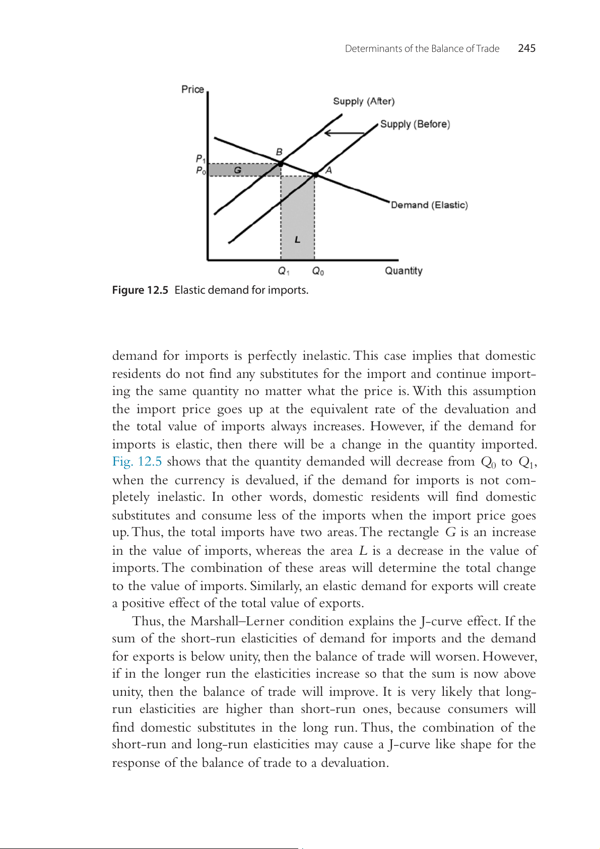
Figure 12.5 Elastic demand for imports.
demand for imports is perfectly inelastic. This case implies that domestic
residents do not find any substitutes for the import and continue import-
ing the same quantity no matter what the price is. With this assumption
the import price goes up at the equivalent rate of the devaluation and
the total value of imports always increases. However, if the demand for
imports is elastic, then there will be a change in the quantity imported.
Fig. 12.5 shows that the quantity demanded will decrease from Q to 0 Q1,
when the currency is devalued, if the demand for imports is not com-
pletely inelastic. In other words, domestic residents will find domestic
substitutes and consume less of the imports when the import price goes
up. Thus, the total imports have two areas. The rectangle G is an increase
in the value of imports, whereas the area L is a decrease in the value of
imports. The combination of these areas will determine the total change
to the value of imports. Similarly, an elastic demand for exports will create
a positive effect of the total value of exports.
Thus, the Marshall–Lerner condition explains the J-curve effect. If the
sum of the short-run elasticities of demand for imports and the demand
for exports is below unity, then the balance of trade will worsen. However,
if in the longer run the elasticities increase so that the sum is now above
unity, then the balance of trade will improve. It is very likely that long-
run elasticities are higher than short-run ones, because consumers will
find domestic substitutes in the long run. Thus, the combination of the
short-run and long-run elasticities may cause a J-curve like shape for the
response of the balance of trade to a devaluation. 246
International Money and Finance
THE EVIDENCE FROM DEVALUATIONS
The preceding discussion has shown the possible short-run effects of a
devaluation on the trade balance through the currency contract and pass-
through periods. What does the evidence of past devaluations have to offer
regarding the actual effects? Unfortunately, the available evidence suggests
that the effects of devaluation appear to differ across countries and time so
that no strong generalizations are possible.
Some authors show that devaluation improves the trade account in the
short run, while others disagree. The reasons for such disagreement come
from the fact that different researchers use different sample periods and
different statistical methodology. Several researchers have focused on the
manner in which producers in different countries adjust the profit mar-
gins on exports to partially offset the effect of exchange rate changes. This
appears to be an important factor in explaining differences in the pass-
through effect across countries. For instance, if the Japanese yen appreci-
ates against the US dollar, the yen appreciation would tend to be passed
through to US importers as a higher dollar price of Japanese exports.
Japanese exporters could limit this pass through of higher prices by reduc-
ing the profit margins on their products and lowering the yen price to
counter the effect of the yen appreciation. This pricing to market behavior
has been found to be especially prevalent among Japanese and German
exporters but is much less common among US exporters. For example,
Gagnon and Knetter (1995) analyzed automobile trade and estimated that
a 10% depreciation of the dollar against the yen would result in Japanese
auto firms reducing their prices so that the dollar price to US import-
ers would rise by only 2.2%. There was no similar evidence of US auto
firms reducing prices for exported autos in response to dollar appreciation.
Klitgaard (1996) found that Japanese exporters tend to lower their profit
margins on exports by 4% (relative to margins on domestic sales) for every
10% appreciation of the yen. He also showed that in addition to cutting
profit margins, in the 1990s Japanese exporters responded to yen apprecia-
tion by shifting production to high-valued products that are less sensitive
to price increases. The Japanese resistance to allowing pass-through effects
is another reason why the Japanese balance of trade may be less responsive
to exchange rate changes than the US trade balance.
There is some evidence that the impact of devaluations may differ over
the short run and long run depending upon what happens to labor costs
relative to the cost of capital. Forbes (2002) has found that in the short
Determinants of the Balance of Trade 247
run following a devaluation, firm output and exports tend to rise as the
cost of labor in the devaluing country falls and firms take advantage of
this to expand production and increase their export sales. However, over
time, capital becomes more expensive to firms in the devaluing country if
the risk associated with that country rises or interest rates rise. So the net
effect of devaluation depends upon the mix of capital and labor utilized in
a nation’s export industries. The evidence from a cross section of countries
suggests that in countries where the ratio of capital to labor employed is
low, devaluations are much more likely to result in export expansion and
faster economic growth. But in countries where the capital/labor ratio is
high, devaluations will tend to have little if any expansionary influence on exports and economic growth.
ABSORPTION APPROACH TO THE BALANCE OF TRADE
The elasticities approach showed that it is possible for a country to
improve its balance of trade through devaluation. Once the exchange rate
effects pass through to import and export prices, imports should fall while
exports increase, stimulating production of goods and services and income
at home. However, this does not always seem to occur. If a country is at
the full-employment level of output prior to the devaluation, then it is
already producing all it can so that no further output can be forthcoming.
What happens in this case following a devaluation? We now turn to the
absorption approach to the balance of trade to answer this question.
The absorption approach to the balance of trade is a theory that emphasizes
how domestic spending on domestic goods changes relative to domestic
output. In other words, the balance of trade is viewed as the difference
between what the economy produces and what it takes, or absorbs, for
domestic use. As commonly treated in introductory economics classes, we
can write total output, Y, as being equal to total expenditures, or
Y = C + I + G + X ( − M ) (12.2)
where C is consumption; I, investment; G, government spending; X,
exports; and M, imports. We can define absorption, A, as being equal to
C + I + G, and net exports as (X − M). Thus we can write:
Y = A + X − M or
Y − A = X − M (12.3) 248
International Money and Finance
Absorption, A, is supposed to represent total domestic spending. Thus,
if total domestic production, ,
Y exceeds absorption (the amount of the
output consumed at home), then the nation will export the rest of its out-
put and run a balance of trade surplus. In contrast, if absorption exceeds
domestic production, then Y − A will be negative; thus by Eq. (12.3),
we note that X − M will also be negative, which has the common-sense
interpretation that the excess of domestic demand over domestic produc-
tion will be met through imports.
The analysis of the absorption approach is really broken down into
two categories, depending upon whether the economy is at its full-
employment level or has unemployed resources. At the full employment, all
resources are being used so that the only way for net exports to increase is
to have absorption fall. On the other hand, with unemployment, Y is not
at its maximum possible value, and thus
Y could increase due to increases
in exports, X, without changing the domestic absorption, A.
The absorption approach is generally concerned with the effects of
a devaluation on the trade balance. If we begin from the case of unem-
ployed resources, we know that domestic output, ,
Y could increase, so that
a devaluation would tend to increase net exports (if the elasticity condi-
tions discussed in the previous section are satisfied) and bring about an
increase in output (given a constant absorption). If we start from , Y at the
full-employment level, it will not be possible to produce more goods and
services. If we devalue, then net exports will tend to increase and the result
is strictly inflation. When foreigners try to spend more on our domestic
production, and yet there is no increase in output forthcoming, the only
result will be a bidding-up of the prices of the goods and services cur- rently being produced.
In the past chapter, we discussed how the IMF has been criticized for
imposing conditions that restrict economic growth and lower living stan-
dards in borrowing countries. The typical conditionality involves reducing
government spending, raising taxes, and restricting money growth. Note
that these types of policies are exactly what the absorption approach pre-
scribes. To increase the likelihood of paying back loans, countries need to
decrease A. Such policies may be interpreted as austerity imposed by the
IMF, but they are intended to reduce A, to make the country more likely
to pay back international loans.
Of course, we must realize that the absorption approach is providing a
theory of the balance of trade, as did the elasticities approach. The absorp-
tion approach can be viewed as a theory of the balance of payments only
in a world without capital flows.
Determinants of the Balance of Trade 249 SUMMARY
1. This chapter discussed why the domestic currency devaluation does
not necessarily improve the balance of trade, especially in the short run.
2. The elasticity of demand (supply) describes how responsive the quan-
tities demanded (supplied) are to a change in price.
3. The elasticities approach to the balance of trade explains how various
degrees of elasticities of demand and supply of imported goods could affect the balance of trade.
4. A devaluation of the domestic currency raises the price of foreign
goods relative to the domestic goods. As prices of imports are increas-
ing, the total payments to importers could rise or fall depending on
the elasticities of demand for imports.
5. The J-curve describes the pattern of the balance of trade after the
currency devaluation such that the trade balance falls in the begin- ning and then rises later.
6. The J-curve effect could be a result of currency contract period and pass-through price adjustment.
7. Since some international exchange contracts are signed before and
the payments are collected after the currency devaluation, the devalu-
ation could worsen the balance of trade when the export contracts
are written in domestic currency and the import contracts are writ- ten in foreign currency.
8. The balance of trade will worsen from a currency devaluation, if
there is a full pass-through, resulting in higher import prices and lower export prices.
9. The Marshall–Lerner condition indicates that if the sum of abso-
lute values of the elasticities of demand for imports and demand for
exports is greater than one, a currency devaluation could improve the balance of trade.
10. Empirically, there is no consensus whether devaluation of a currency
can improve the trade account in the short run.
11. The domestic absorption is the total domestic spending on domesti-
cally produced goods by consumers, business firms, and government.
12. According to the absorption approach, the effects of the cur-
rency devaluation on trade balance depend not only on whether an
economy is operating at its full employment, but also whether the
domestic absorption changes during the devaluation. At the full-
employment level, if the domestic absorption remains constant, the
currency devaluation will not change the balance of trade. 250
International Money and Finance EXERCISES
1. Suppose that the United States is considering devaluing its dollar
against a foreign currency to improve the trade balance. What type of
currency contracting would have a negative effect on the trade balance?
2. Suppose that the United States is considering devaluing its dollar
against a foreign currency to improve the trade balance. What type
of pass-through effects would lead to a positive effect on the trade balance?
3. Suppose that the United States is considering devaluing its dol-
lar against a foreign currency to improve the trade balance. Use the
absorption approach to explain how the United States can improve its
trade balance from the currency devaluation, if the country is currently
operating in the full-employment level of output.
4. Give examples of policies that a country could implement to reduce its absorption.
5. What is the J-curve? Explain.
6. How can we use the Marshall–Lerner condition to explain the J-curve effect? FURTHER READING
Allen, M., 2006. Exchange Rates and Trade Balance Adjustment in Emerging Market
Economies. International Monetary Fund. October.
Baek, J., Koo, W.W., Mulik, K., 2009. Exchange rate dynamics and the bilateral trade balance:
the case of U.S. agriculture. Agr. Resour. Econ. Rev. 38 (2), 213–228.
Devereaux, M.B., 2000. How does a devaluation affect the current account? J. Int. Money Financ. 19 (6), 833–851.
Devereux, M.B., Engel, C., Storgaard, P.E., 2004. Endogenous exchange rate pass-through
when nominal prices are set in advance. J. Int. Econ. 63 (2), 263–291.
Forbes, K., 2002. Cheap labor meets costly capital: the impact of devaluations on commodity
firms. J. Dev. Econ. 69, 335–365.
Gagnon, J.E., Knetter, M.M., 1995. Markup adjustment and exchange rate fluctuations:
evidence from panel data on automobile exports. J. Int. Money Financ. April.
Gopinath, G., Itskhoki, O., Rigobon, R., 2010. Currency choice and exchange rate pass-
through. Am. Econ. Rev. 100 (1), 304–336.
Klitgaard, T., 1996. Coping with the rising yen: Japan’s recent export experience. Cur. Issues Econ. Financ. January.
Klitgaard, T., 1999. Exchange rates and profit margins: the case of Japanese exporters.
FRBNY Econ. Policy Rev. April.
Koray, F., McMillin, W.D., 1999. Monetary shocks, the exchange rate, and the trade balance.
J. Int. Money Financ. December.
Rose, A., 1991. The role of exchange rates in a popular model of international trade: does
the ‘Marshall–Lerner condition’ hold? J. Int. Econ. 3–4, 301–316.
Rose, A., 1996. Are all devaluations alike? FRBSF Econ. Lett. February.
Tài liệu liên quan:
-

Hoạt động Tài chính của Doanh nghiệp Đa Quốc Gia (DN) - Chương 6 | Tài chính quốc tế | Trường Học Viện nông nghiệp Việt Nam
19 10 -

Hệ Thống Tiền Tệ Quốc Tế: Khái Niệm và Các Chế Độ Tỷ Giá | Tài chính quốc tế | Trường Học Viện nông nghiệp Việt Nam
24 12 -

Bài giảng Chương 1: Các Quan Hệ Cân Bằng Quốc Tế và LOP | Tài chính quốc tế | Trường Học Viện nông nghiệp Việt Nam
21 11 -
Cách Tính Lạm Phát và CPI: So Sánh Việt Nam và Mỹ | Tài chính quốc tế | Trường Học Viện nông nghiệp Việt Nam
23 12 -

Detailed Report and Analysis on Submission Trends | Tài chính quốc tế | Trường Học Viện nông nghiệp Việt Nam
23 12