Essentials of Economics: Natural Monopoly Insights | Microeconomics | Trường Đại học Quốc tế, Đại học Quốc gia Thành phố Hồ Chí Minh
An industry is a natural monopoly when a single firm can supply a market with a good or service at a lower cost than two or more firms could. This happens when there are economies of scale over the relevant range of output. Figure 1 shows the average total costs of a firm with economies of scale. In this case, a single firm can produce any amount of output at the lowest cost. That is, for any given amount of output, a larger number of firms leads to less output per firm and higher average total cost. Tài liệu được sưu tầm và soạn thảo dưới dạng file PDF để gửi tới các bạn cùng tham khảo, ôn tập đầy đủ kiến thức, chuẩn bị cho các buổi học thật tốt. Mời bạn đọc đón xem!
Môn: Microeconomics 245 tài liệu
Trường: Trường Đại học Quốc tế, Đại học Quốc gia Thành phố Hồ Chí Minh 1.5 K tài liệu
Tác giả:


Preview text:
274
Part V Firm Behavior and the Organization of Industry
14-1c Natural Monopolies natural monopoly
An industry is a natural monopoly when a single firm can supply a market with a a type of monopoly that
good or service at a lower cost than two or more firms could. This happens when arises because a single
there are economies of scale over the relevant range of output. Figure 1 shows the firm can supply a good
average total costs of a firm with economies of scale. In this case, a single firm can or service to an entire
produce any amount of output at the lowest cost. That is, for any given amount of market at a lower cost
output, a larger number of firms leads to less output per firm and higher average than could two or more total cost. firms
The distribution of tap water is an example of a natural monopoly. To provide
water to town residents, a firm must build a network of pipes. If two or more firms
were to compete, each would have to incur the fixed cost of building a network.
The average total cost is lowest if a single firm provides water to the entire market.
Other examples of natural monopolies appeared in Chapter 11, which noted that
club goods are excludable but not rival in consumption. An example is a bridge used
so rarely that it is never congested. The bridge is excludable because a toll collector
can prevent someone from using it. The bridge is not rival in consumption because
one person’s use of the bridge does not hinder others’ use of it. There is a large
fixed cost of building the bridge but a negligible marginal cost of additional users,
so the average total cost (the total cost divided by the number of trips) declines as
the number of trips rises, making the bridge a natural monopoly.
When a firm is a natural monopoly, it is less concerned about new entrants eroding
its monopoly power. Normally, a firm has trouble maintaining a monopoly position
without government protection or ownership of a key resource. The monopolist’s
profit attracts entrants into the market, and these entrants make the market more
competitive. By contrast, entering a market in which another firm has a natural
monopoly is unattractive. Would-be entrants know that they cannot achieve the
same low costs that the monopolist enjoys because, after entry, each firm would
have a smaller piece of the market.
In some cases, the size of the market determines whether an industry is a natural
monopoly. Again, consider a bridge across a river. When the population is small,
the bridge may be a natural monopoly. A single bridge can meet the entire demand Figure 1 Cost
Economies of Scale as a Cause of Monopoly
When a firm’s average-total-cost
curve continually declines, the
firm has what is called a natural monopoly. In this case, when
production is divided among more
firms, each firm produces less, and
average total cost rises. As a result, Average a single firm can produce any total
given amount at the lowest cost. cost 0 Quantity of Output Chapter 14 Monopoly 275
for trips across the river at the lowest cost. Yet as the population grows and the
bridge becomes congested, meeting demand may require multiple bridges. As the
market expands, the natural monopoly can evolve into a more competitive market. QuickQuiz
1. Some government grants of monopoly power may be
2. A firm is a natural monopoly if it exhibits ________ desirable if they as its output increases.
a. curtail the adverse effects of cut-throat a. increasing total revenue competition. b. increasing marginal cost
b. make industries more profitable. c. decreasing marginal revenue
c. provide incentives for invention and artistic
d. decreasing average total cost creation.
d. save consumers from having to choose among alternative suppliers.
Answers are at the end of the chapter.
14-2 How Monopolies Make Production and Pricing Decisions
Having seen how monopolies arise, let’s consider how a monopoly firm decides
how much to produce and what price to charge. The analysis of monopoly behavior
in this section is the starting point for evaluating whether monopolies are desirable
and what policies a government might pursue in monopoly markets.
14-2a Monopoly versus Competition
The key difference between a competitive firm and a monopoly is the monopoly’s
ability to influence the price of its output. A competitive firm is small relative to
the market in which it operates and, therefore, has no power to influence the price
of its output. It takes the price as given by market conditions. By contrast, because
a monopoly is the sole producer in its market, it can alter the price of its good by
adjusting the quantity it supplies.
One way to view this difference between a competitive firm and a monopoly is
to consider the demand curve that each faces. In the analysis of competitive firms
in the preceding chapter, we drew the market price as a horizontal line. Because a
competitive firm can sell as much or as little as it wants at this price, the competitive
firm faces a horizontal demand curve, as in panel (a) of Figure 2. In effect, because
the competitive firm sells a product with many perfect substitutes (the products of all
the other firms in its market), the demand curve for any one firm is perfectly elastic.
By contrast, because a monopoly is the sole producer in its market, its demand
curve is simply the market demand curve, which slopes downward, as in panel (b)
of Figure 2. If the monopolist raises the price of its good, consumers buy less of it.
Put another way, if the monopolist reduces the quantity of output it produces and
sells, the price of its output increases.
The market demand curve provides a constraint on a monopoly’s ability to profit
from its market power. A monopolist would prefer to charge a high price and sell a
large quantity at that high price. But its demand curve makes that outcome impos-
sible. The market demand curve describes the combinations of price and quantity 276
Part V Firm Behavior and the Organization of Industry Figure 2
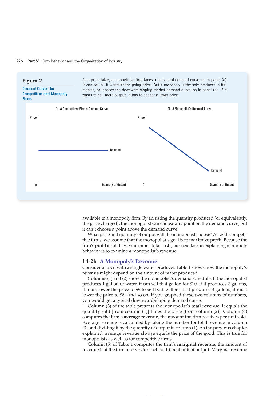
As a price taker, a competitive firm faces a horizontal demand curve, as in panel (a).
It can sell all it wants at the going price. But a monopoly is the sole producer in its Demand Curves for
market, so it faces the downward-sloping market demand curve, as in panel (b). If it
Competitive and Monopoly
wants to sell more output, it has to accept a lower price. Firms
(a) A Competitive Firm’s Demand Curve
(b) A Monopolist’s Demand Curve Price Price Demand Demand 0 Quantity of Output 0 Quantity of Output
available to a monopoly firm. By adjusting the quantity produced (or equivalently,
the price charged), the monopolist can choose any point on the demand curve, but
it can’t choose a point above the demand curve.
What price and quantity of output will the monopolist choose? As with competi-
tive firms, we assume that the monopolist’s goal is to maximize profit. Because the
firm’s profit is total revenue minus total costs, our next task in explaining monopoly
behavior is to examine a monopolist’s revenue.
14-2b A Monopoly’s Revenue
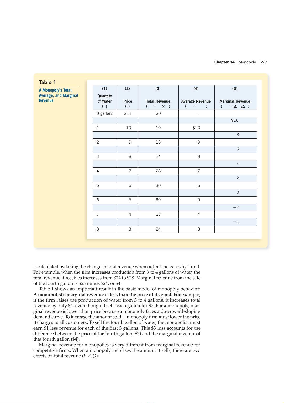
Consider a town with a single water producer. Table 1 shows how the monopoly’s
revenue might depend on the amount of water produced.
Columns (1) and (2) show the monopolist’s demand schedule. If the monopolist
produces 1 gallon of water, it can sell that gallon for $10. If it produces 2 gallons,
it must lower the price to $9 to sell both gallons. If it produces 3 gallons, it must
lower the price to $8. And so on. If you graphed these two columns of numbers,
you would get a typical downward-sloping demand curve.
Column (3) of the table presents the monopolist’s total revenue. It equals the
quantity sold [from column (1)] times the price [from column (2)]. Column (4)
computes the firm’s average revenue, the amount the firm receives per unit sold.
Average revenue is calculated by taking the number for total revenue in column
(3) and dividing it by the quantity of output in column (1). As the previous chapter
explained, average revenue always equals the price of the good. This is true for
monopolists as well as for competitive firms.
Column (5) of Table 1 computes the firm’s marginal revenue, the amount of
revenue that the firm receives for each additional unit of output. Marginal revenue Chapter 14 Monopoly 277 Table 1 A Monopoly’s Total, (1) (2) (3) (4) (5) Average, and Marginal Quantity Revenue of Water Price Total Revenue Average Revenue Marginal Revenue (Q) (P) (TR 5 P 3 Q) (AR 5 TR/Q) (MR 5 DTR/DQ) 0 gallons $11 $0 — $10 1 10 10 $10 8 2 9 18 9 6 3 8 24 8 4 4 7 28 7 2 5 6 30 6 0 6 5 30 5 22 7 4 28 4 24 8 3 24 3
is calculated by taking the change in total revenue when output increases by 1 unit.
For example, when the firm increases production from 3 to 4 gallons of water, the
total revenue it receives increases from $24 to $28. Marginal revenue from the sale
of the fourth gallon is $28 minus $24, or $4.
Table 1 shows an important result in the basic model of monopoly behavior:
A monopolist’s marginal revenue is less than the price of its good. For example,
if the firm raises the production of water from 3 to 4 gallons, it increases total
revenue by only $4, even though it sells each gallon for $7. For a monopoly, mar-
ginal revenue is lower than price because a monopoly faces a downward-sloping
demand curve. To increase the amount sold, a monopoly firm must lower the price
it charges to all customers. To sell the fourth gallon of water, the monopolist must
earn $1 less revenue for each of the first 3 gallons. This $3 loss accounts for the
difference between the price of the fourth gallon ($7) and the marginal revenue of that fourth gallon ($4).
Marginal revenue for monopolies is very different from marginal revenue for
competitive firms. When a monopoly increases the amount it sells, there are two
effects on total revenue (P 3 Q): 278
Part V Firm Behavior and the Organization of Industry ●
The output effect: More output is sold, so Q is higher, which increases total revenue. ●
The price effect: The price falls, so P is lower, which decreases total revenue.
Because a competitive firm can sell all it wants at the market price, there is no price
effect. When it increases production by 1 unit, it receives the market price for that
unit, and it does not receive any less for the units it was already selling. That is,
because the competitive firm is a price taker, its marginal revenue equals the price
of its good. By contrast, when a monopoly increases production by 1 unit, it must
reduce the price it charges for every unit it sells, and this price cut reduces revenue
from the units it was already selling. As a result, a monopoly’s marginal revenue is less than its price.
Figure 3 graphs the demand curve and the marginal-revenue curve for a
monopoly. (Because the monopoly’s price equals its average revenue, the demand
curve is also the average-revenue curve.) These two curves always start at the same
point on the vertical axis because the marginal revenue of the first unit sold equals
the price of the good. But for the reason just discussed, the monopolist’s marginal
revenue on all units after the first is less than the price. That’s why a monopoly’s
marginal-revenue curve lies below its demand curve.
You can see in Figure 3 (as well as in Table 1) that marginal revenue can even
become negative. That happens when the price effect on revenue outweighs the
output effect. In this case, an additional unit of output causes the price to fall by
enough that the firm, despite selling more units, receives less revenue. 14-2c Profit Maximization
Now that we have considered the revenue of a monopoly firm, we are ready to
examine how such a firm maximizes profit. Recall from Chapter 1 that one of the
Ten Principles of Economics is that rational people think at the margin. This lesson
is as true for monopolists as it is for competitive firms. Here, we apply the logic of
marginal analysis to the monopolist’s decision about how much to produce. Figure 3 Price
Demand and Marginal-Revenue $11 Curves for a Monopoly 10
The demand curve shows how the 9
quantity sold affects the price. The 8
marginal-revenue curve shows how 7
the firm’s revenue changes when 6
the quantity increases by 1 unit. 5
Because the price on all units sold 4
must fall if the monopoly increases 3 Demand
production, marginal revenue is 2 Marginal (average revenue less than the price. 1 revenue) 0 21 1 2 3 4 5 6 7 8 Quantity of Water 22 23 24 Chapter 14 Monopoly 279 Figure 4 Costs and
Profit Maximization for a Monopoly Revenue 2. . . . and then the demand 1. The intersection of the
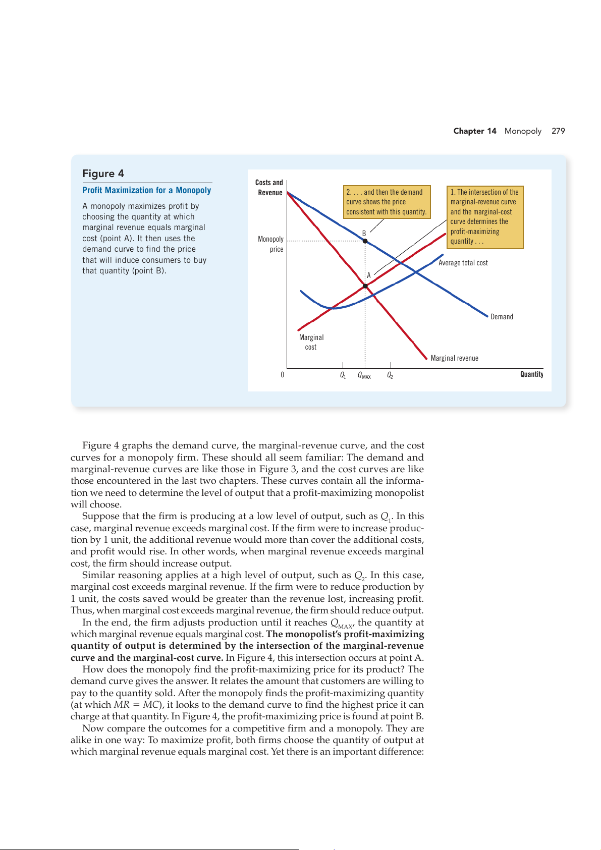
A monopoly maximizes profit by curve shows the price marginal-revenue curve
choosing the quantity at which consistent with this quantity. and the marginal-cost curve determines the
marginal revenue equals marginal profit-maximizing
cost (point A). It then uses the B Monopoly quantity . . .
demand curve to find the price price
that will induce consumers to buy Average total cost that quantity (point B). A Demand Marginal cost Marginal revenue 0 Q Q Quantity 1 MAX Q2
Figure 4 graphs the demand curve, the marginal-revenue curve, and the cost
curves for a monopoly firm. These should all seem familiar: The demand and
marginal-revenue curves are like those in Figure 3, and the cost curves are like
those encountered in the last two chapters. These curves contain all the informa-
tion we need to determine the level of output that a profit-maximizing monopolist will choose.
Suppose that the firm is producing at a low level of output, such as Q . In this 1
case, marginal revenue exceeds marginal cost. If the firm were to increase produc-
tion by 1 unit, the additional revenue would more than cover the additional costs,
and profit would rise. In other words, when marginal revenue exceeds marginal
cost, the firm should increase output.
Similar reasoning applies at a high level of output, such as Q . In this case, 2
marginal cost exceeds marginal revenue. If the firm were to reduce production by
1 unit, the costs saved would be greater than the revenue lost, increasing profit.
Thus, when marginal cost exceeds marginal revenue, the firm should reduce output.
In the end, the firm adjusts production until it reaches Q , the quantity at MAX
which marginal revenue equals marginal cost. The monopolist’s profit-maximizing
quantity of output is determined by the intersection of the marginal-revenue
curve and the marginal-cost curve. In Figure 4, this intersection occurs at point A.
How does the monopoly find the profit-maximizing price for its product? The
demand curve gives the answer. It relates the amount that customers are willing to
pay to the quantity sold. After the monopoly finds the profit-maximizing quantity
(at which MR 5 MC), it looks to the demand curve to find the highest price it can
charge at that quantity. In Figure 4, the profit-maximizing price is found at point B.
Now compare the outcomes for a competitive firm and a monopoly. They are
alike in one way: To maximize profit, both firms choose the quantity of output at
which marginal revenue equals marginal cost. Yet there is an important difference: 280
Part V Firm Behavior and the Organization of Industry
Why a Monopoly Does Not Have a Supply Curve
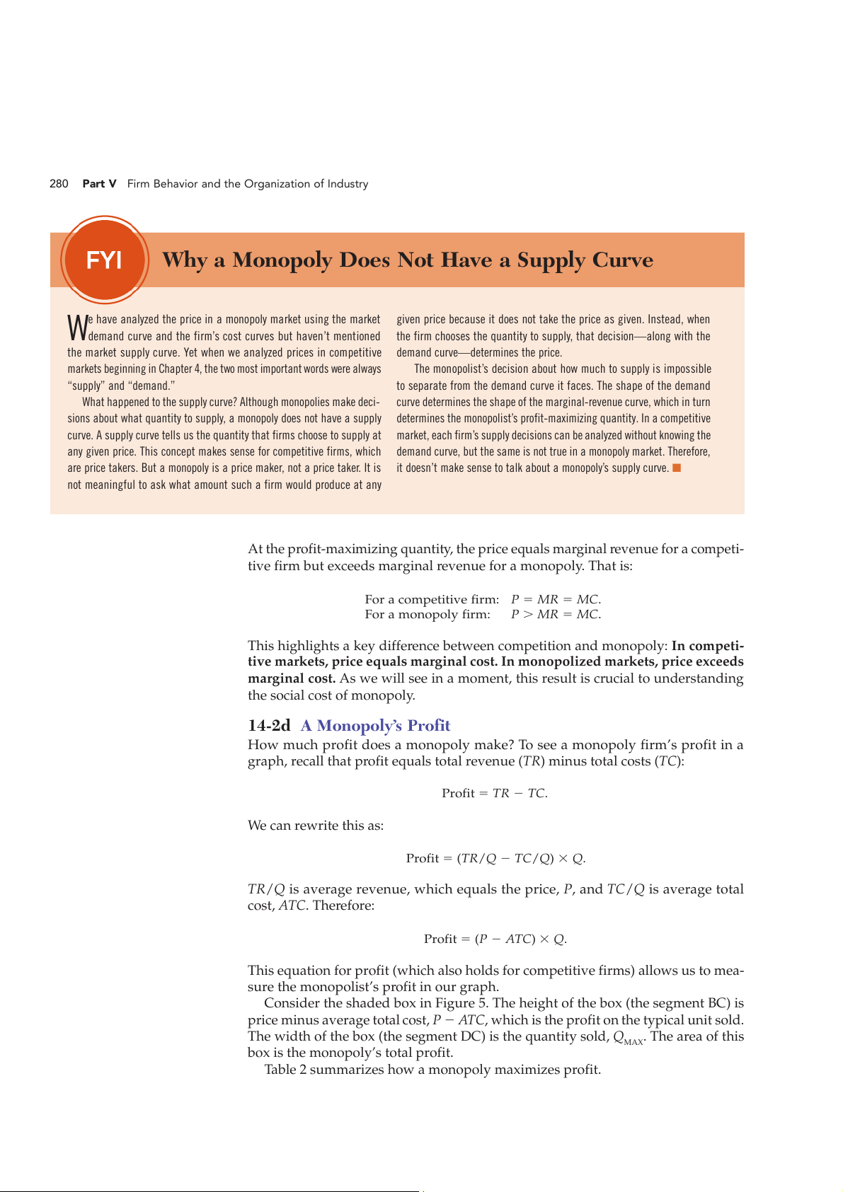
given price because it does not take the price as given. Instead, when
We have analyzed the price in a monopoly market using the market
demand curve and the firm’s cost curves but haven’t mentioned the firm chooses the quantity to supply, that decision—along with the
the market supply curve. Yet when we analyzed prices in competitive demand curve—determines the price.
markets beginning in Chapter 4, the two most important words were always
The monopolist’s decision about how much to supply is impossible “supply” and “demand.”
to separate from the demand curve it faces. The shape of the demand
What happened to the supply curve? Although monopolies make deci-
curve determines the shape of the marginal-revenue curve, which in turn
sions about what quantity to supply, a monopoly does not have a supply determines the monopolist’s profit-maximizing quantity. In a competitive
curve. A supply curve tel s us the quantity that firms choose to supply at market, each firm’s supply decisions can be analyzed without knowing the
any given price. This concept makes sense for competitive firms, which demand curve, but the same is not true in a monopoly market. Therefore,
are price takers. But a monopoly is a price maker, not a price taker. It is it doesn’t make sense to talk about a monopoly’s supply curve. ■
not meaningful to ask what amount such a firm would produce at any
At the profit-maximizing quantity, the price equals marginal revenue for a competi-
tive firm but exceeds marginal revenue for a monopoly. That is:
For a competitive firm: P 5 MR 5 MC. For a monopoly firm:
P . MR 5 MC.
This highlights a key difference between competition and monopoly: In competi-
tive markets, price equals marginal cost. In monopolized markets, price exceeds
marginal cost. As we will see in a moment, this result is crucial to understanding the social cost of monopoly. 14-2d A Monopoly’s Profit
How much profit does a monopoly make? To see a monopoly firm’s profit in a
graph, recall that profit equals total revenue (TR) minus total costs (TC):
Profit 5 TR 2 TC. We can rewrite this as:
Profit 5 (TR/Q 2 TC/Q) 3 Q.
TR/Q is average revenue, which equals the price, P, and TC/Q is average total cost, ATC. Therefore:
Profit 5 (P 2 ATC) 3 Q.
This equation for profit (which also holds for competitive firms) allows us to mea-
sure the monopolist’s profit in our graph.
Consider the shaded box in Figure 5. The height of the box (the segment BC) is
price minus average total cost, P 2 ATC, which is the profit on the typical unit sold.
The width of the box (the segment DC) is the quantity sold, Q . The area of this MAX
box is the monopoly’s total profit.
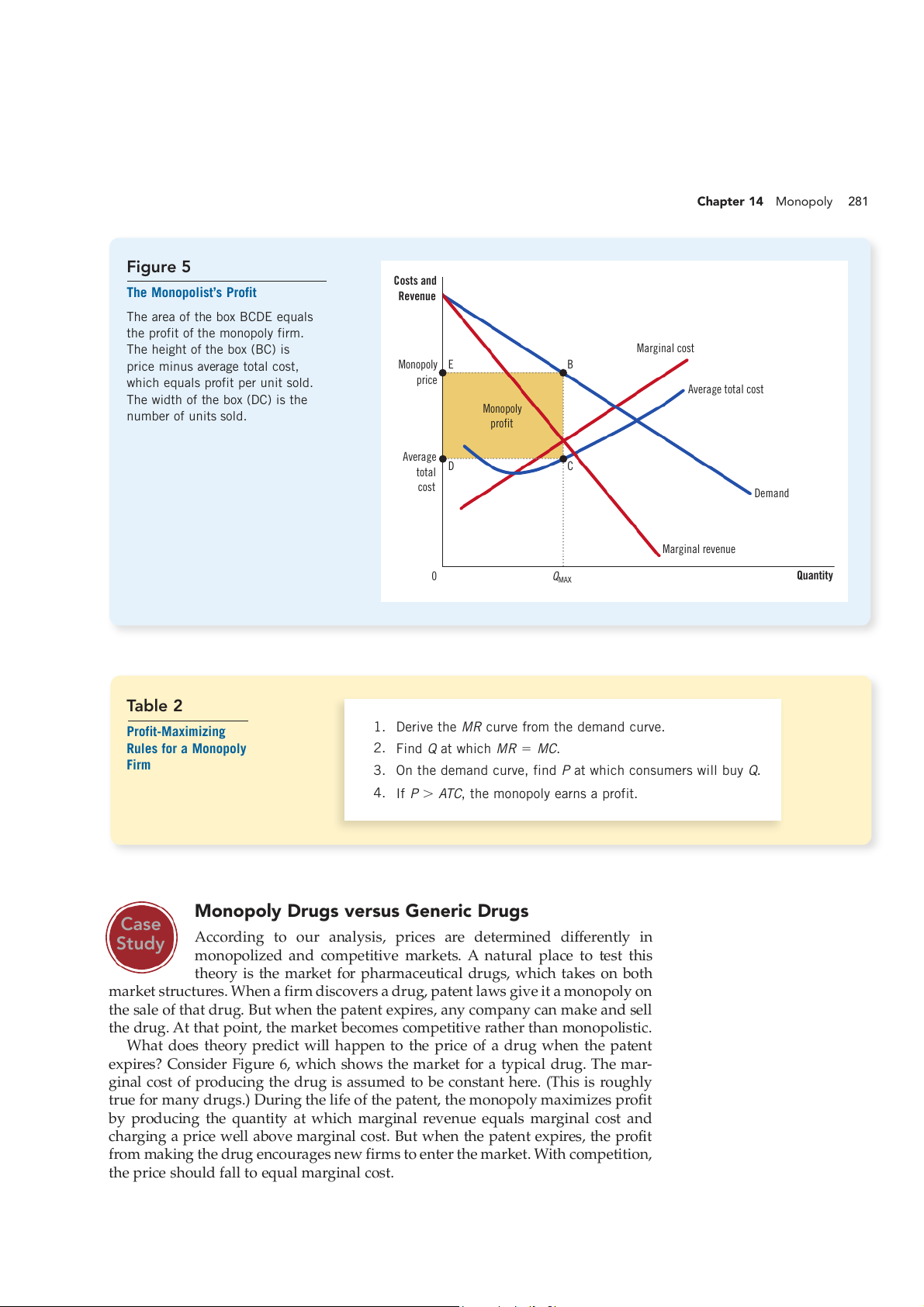
Table 2 summarizes how a monopoly maximizes profit. Chapter 14 Monopoly 281 Figure 5 Costs and
The Monopolist’s Profit Revenue
The area of the box BCDE equals
the profit of the monopoly firm. The height of the box (BC) is Marginal cost
price minus average total cost, Monopoly E B
which equals profit per unit sold. price Average total cost
The width of the box (DC) is the number of units sold. Monopoly profit Average total D C cost Demand Marginal revenue 0 Q Quantity MAX Table 2 Profit-Maximizing
1. Derive the MR curve from the demand curve. Rules for a Monopoly 2. Find Q at which MR 5 MC. Firm
3. On the demand curve, find P at which consumers will buy Q.
4. If P . ATC, the monopoly earns a profit.
Monopoly Drugs versus Generic Drugs Case Study
According to our analysis, prices are determined differently in
monopolized and competitive markets. A natural place to test this
theory is the market for pharmaceutical drugs, which takes on both
market structures. When a firm discovers a drug, patent laws give it a monopoly on
the sale of that drug. But when the patent expires, any company can make and sell
the drug. At that point, the market becomes competitive rather than monopolistic.
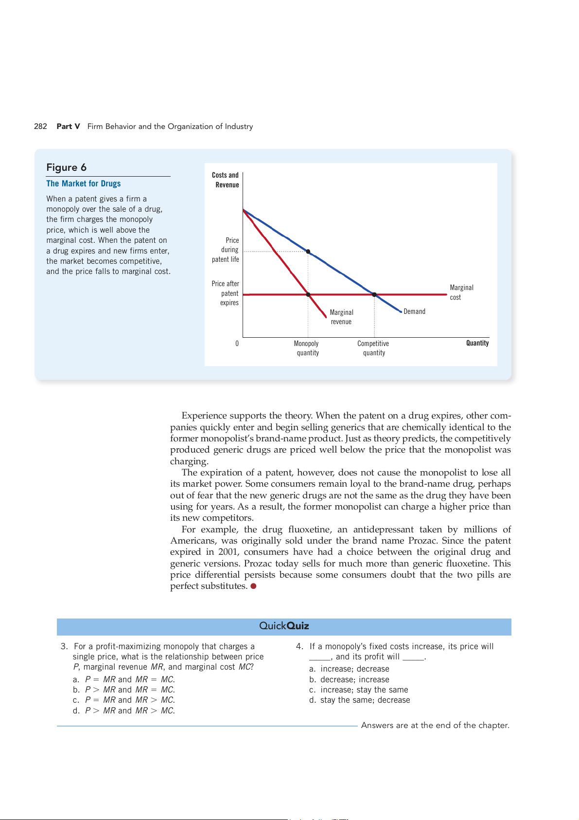
What does theory predict will happen to the price of a drug when the patent
expires? Consider Figure 6, which shows the market for a typical drug. The mar-
ginal cost of producing the drug is assumed to be constant here. (This is roughly
true for many drugs.) During the life of the patent, the monopoly maximizes profit
by producing the quantity at which marginal revenue equals marginal cost and
charging a price well above marginal cost. But when the patent expires, the profit
from making the drug encourages new firms to enter the market. With competition,
the price should fall to equal marginal cost. 282
Part V Firm Behavior and the Organization of Industry Figure 6 Costs and The Market for Drugs Revenue When a patent gives a firm a
monopoly over the sale of a drug, the firm charges the monopoly
price, which is well above the
marginal cost. When the patent on Price
a drug expires and new firms enter, during
the market becomes competitive, patent life
and the price falls to marginal cost. Price after Marginal patent cost expires Marginal Demand revenue 0 Monopoly Competitive Quantity quantity quantity
Experience supports the theory. When the patent on a drug expires, other com-
panies quickly enter and begin selling generics that are chemically identical to the
former monopolist’s brand-name product. Just as theory predicts, the competitively
produced generic drugs are priced well below the price that the monopolist was charging.
The expiration of a patent, however, does not cause the monopolist to lose all
its market power. Some consumers remain loyal to the brand-name drug, perhaps
out of fear that the new generic drugs are not the same as the drug they have been
using for years. As a result, the former monopolist can charge a higher price than its new competitors.
For example, the drug fluoxetine, an antidepressant taken by millions of
Americans, was originally sold under the brand name Prozac. Since the patent
expired in 2001, consumers have had a choice between the original drug and
generic versions. Prozac today sells for much more than generic fluoxetine. This
price differential persists because some consumers doubt that the two pills are perfect substitutes.● QuickQuiz
3. For a profit-maximizing monopoly that charges a
4. If a monopoly’s fixed costs increase, its price will
single price, what is the relationship between price
_____, and its profit will _____.
P, marginal revenue MR, and marginal cost MC? a. increase; decrease a. P 5 MR and MR 5 MC. b. decrease; increase b. P . MR and MR 5 MC. c. increase; stay the same c. P 5 MR and MR . MC. d. stay the same; decrease d. P . MR and MR . MC.
Answers are at the end of the chapter.
Tài liệu liên quan:
-
Elasticity Problems and Solutions: Practice Exercises | Microeconomics | Trường Đại học Quốc tế, Đại học Quốc gia Thành phố Hồ Chí Minh
5 3 -
Supply and Demand - ôn tập: Market Equilibrium Effects Analysis | Microeconomics | Trường Đại học Quốc tế, Đại học Quốc gia Thành phố Hồ Chí Minh
3 2 -
Monopoly & Monopolistic Competition | Microeconomics | Trường Đại học Quốc tế, Đại học Quốc gia Thành phố Hồ Chí Minh
4 2 -
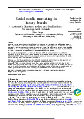
Systematic Review of Social Media Marketing in Luxury Brands | Microeconomics | Trường Đại học Quốc tế, Đại học Quốc gia Thành phố Hồ Chí Minh
4 2 -
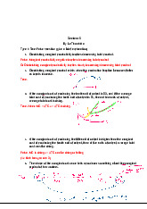
Seminar-5: Economics | Microeconomics | Trường Đại học Quốc tế, Đại học Quốc gia Thành phố Hồ Chí Minh
4 2