
Exercise 2 instruction - Business Computing Skills | Trường Đại học Quốc tế, Đại học Quốc gia Thành phố HCM

Exercise 2 instruction - Business Computing Skills | Trường Đại học Quốc tế, Đại học Quốc gia Thành phố HCM được sưu tầm và soạn thảo dưới dạng file PDF để gửi tới các bạn sinh viên cùng tham khảo, ôn tập đầy đủ kiến thức, chuẩn bị cho các buổi học thật tốt. Mời bạn đọc đón xem!

Thông tin:
11 trang 7 tháng trước

Bình luận

Vui lòng đăng nhập hoặc đăng ký để gửi bình luận.

Exercise 2 instruction - Business Computing Skills | Trường Đại học Quốc tế, Đại học Quốc gia Thành phố HCM

Exercise 2 instruction - Business Computing Skills | Trường Đại học Quốc tế, Đại học Quốc gia Thành phố HCM được sưu tầm và soạn thảo dưới dạng file PDF để gửi tới các bạn sinh viên cùng tham khảo, ôn tập đầy đủ kiến thức, chuẩn bị cho các buổi học thật tốt. Mời bạn đọc đón xem!

32 16 lượt tải Tải xuống
Open the Exercise 1 excel file.
Exercise 1: Type some simple formulas to add, subtract, multiply,
and divide.
1. Click in cell A1. First you’ll add two numbers.
2. Type =734+498
3. Press ENTER on your keyboard to get the result of 1232.
4. Now let’s subtract, multiply, and divide.
In cell A2, type and press ENTER. Result: 236.=734-498
In cell A3, type and press ENTER. Result: 365532.=734*498
In cell A4, type and press ENTER. Result: 1.4738956. (The answer may=734/498
vary, depending on how many decimal places are set up in your version of Excel.)
5. Click in cell A4 to adjust the number of numerals after the decimal place. Make
sure you are on the tab. If not, click the tab to select it. Home
6. Move the cursor up to the ribbon, where it says (called the Number Number
group).
7. In the group, point to and click. Notice the Number Decrease Decimal
result in cell A4, which should have one less number after the decimal point. Click
Decrease Decimal as many times as you want to adjust the number.
Exercise 2: Add numbers by using AutoSum
In this exercise, Excel will add numbers by creating a formula for you.
1. Click in cell A5.
2. On the tab, move the cursor to where it says (called the Home Editing Editing
group).
3. Click . The formula appears on the spreadsheet. It should include AutoSum
all the cells between cell A1 and cell A4.
4. Press ENTER to get the result: 367001.47.
(The answer may vary, depending on how many decimal places are set up in your version of Excel.)
Exercise 3: For something new, a math shortcut
Sometimes you may want to see a number but not want to use a formula to get the number onto a spreadsheet. You just
want to know the result. Here’s how.
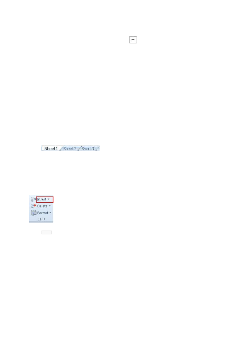
1. First change the spreadsheet you are working on. In the lower-left corner of the
spreadsheet, where it says , , and , click the tab to openSheet1 Sheet2 Sheet3 Sheet2
the spreadsheet.
2. Click in cell A2, where it says $23.75.
3. When you clicked in the cell, you noticed the cursor changed to a white plus sign.
Click and drag the cursor down the column until you get to the end of cell A10.
4. Release the mouse button.
The contents will be highlighted, and there should be a single black line around all the cells, indicating that the cells
are selected.
5. Now look at the status bar, in the lower-right corner of the spreadsheet. What you
see depends on how your version of Excel is set up.
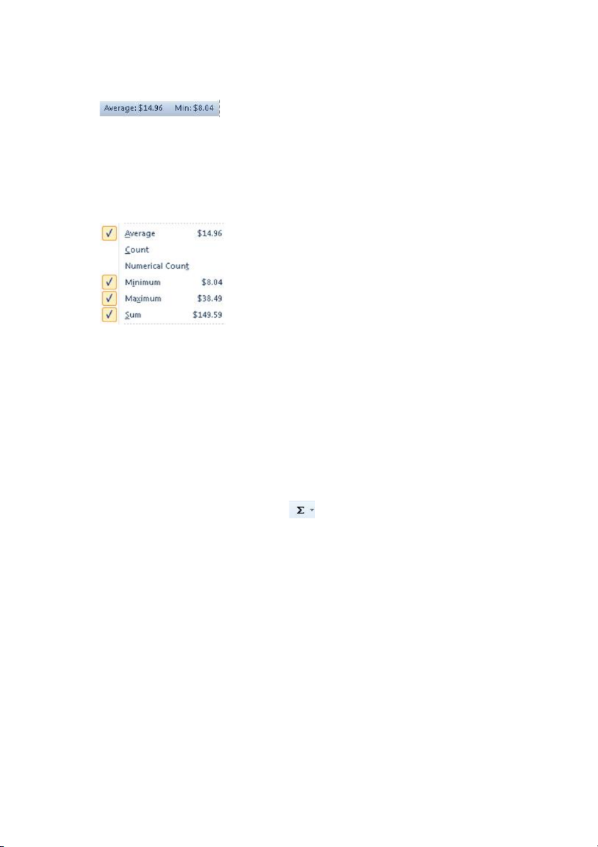
You might see Average: $14.96, Min: $8.04, Max: $38.49, and Sum: $134.63.
6. If you see more than this, that’s fine. If you don’t see all these numbers, with the
cursor on the status bar, right-click the bar. Be sure to click the status bar, not the
horizontal scroll bar that is just above the status bar.
The menu is displayed. Here’s a portion of the menu.Customize Status Bar
7. A check mark means that the function results will appear on the status bar. Click
next to any of the functions for the numbers you’d like to display on the status bar.
Exercise 4: Get an average
When you want a number, such as an average, on your spreadsheet instead of only on the status bar, here’s how to do
that:
1. Still on Sheet2, click in cell A11 (the first cell under the numbers in column A).
2. Move your cursor up to the ribbon, on the tab, to the group. Home Editing
3. Then point the cursor to in the group.AutoSum Editing
4. Click the arrow next to . AutoSum
5. Click Average.
6. Press ENTER or TAB on your keyboard to get the result: $14.96.
7. Repeat the above steps for , , and , Count Numbers Max Min
Exercise 5: Copy a formula
1. Click in cell A11, the cell with the average amount in it.
2. Point to the lower-right corner of the cell, until the cursor changes into a black
plus sign .
3. Click and drag from cell A11 to cell B11. Release the mouse button. The result in
cell B12 is $34.12.
Part Two: Work with column titles
Exercise 1: Create titles and adjust column width
1. Click in cell D1. Then type . It looks as though the name is tooProduct category
long to fit in the cell. Ignore that for now, and press the TAB key.
2. In cell E1, type . Press the TAB key. Customer name
3. In cell F1, type , and press the TAB key.Sales amount
4. In cell G1, type Year, and press the TAB key.
Now you’ll adjust the column widths.
5. Select the title cells by clicking in cell D1 and dragging through cell G1.
6. On the ribbon, in the group, click the arrow next to Cells Format.
NOTE In your version of Excel, the group could look slightly different, depending on screen resolution and Cells
screen size. The arrows can be either next to or under commands.
7. On the menu that appears, click . This makes column AutoFit Column Width
title text readable.
Exercise 2: Format titles
1. The cells should still be selected (highlighted, with a black line around all the
cells). If not, follow step 5 above.)
2. On the ribbon, in the group, click the arrow next to . Styles Cell Styles
3. Move the cursor over the styles in the Style gallery, and notice the style preview
in cells D1 through G1.
If the Style gallery covers all the column titles, you can use the scroll bar at the bottom of the spreadsheet to move
the spreadsheet so that more titles are visible.
4. Click any style you like to apply it to the titles.
If the style makes the text larger, follow the steps in Exercise 1, steps 6 and 7, to automatically adjust the column
widths again.
Exercise 3: Change a column width manually
Sometimes you might want to make a column wider. For example, the Year column is very narrow. That’s fine, but if you
decide that you want it to be wider, you can adjust the column width.
1. Click in cell G1. Then move the cursor up above the cell, to the right border of
“G.” The cursor should turn into a four headed pointer .
2. Click and drag until the column is as wide as you want it to be.
Exercise 4: Center the titles
1. Select the cells by clicking in cell D1 and dragging to the end of cell G1.
2. On the ribbon, in the group, click . Alignment Center
Part Three: Let Excel do some typing for you
Exercise 1: Fill in some text, try AutoComplete, and for something
new, see what to do if Excel guesses incorrectly
1. In cell D2, type Mountain bikes, and then press ENTER to move the cursor down
one cell.
2. In cell D3, type Road bikes and then press ENTER.
3. In cell D4, type .M
Excel assumes you are typing Mountain bikes and fills in everything after the “M” that you typed. That’s correct.
Press ENTER.
4. Now you’ll see what happens if Excel does not correctly guess what you want to
type. In cell D5, type only. R
Excel fills in Road bikes for you. But that’s not correct, because you’re going to type Row boats instead.
5. Just type over what Excel entered for you. The “R” is correct, so after the “R,”
type . Press ENTER. ow boats
6. In cell D6 type a product again, starting with .R
You need to let Excel know which “R” product you want to type. You decide: For Road bikes, type . For Row boats, oa
type . Then press ENTER. ow
In general, when you type words that begin with the same letter or letters, you need to type enough letters for
Excel to recognize which words you want to enter into the cells.
Exercise 2: Let Excel fill in a series for you
1. Click in cell B14.
2. Type a month of the year, any month.
3. Then move the white plus sign cursor to the lower-right corner of the cell, until
the cursor turns into a black plus sign . Click and drag down the column. ScreenTips
display each month that Excel will enter into a cell.
4. When you’ve dragged as much as you want to, release the mouse button. Excel
fills in the series for you.
Exercise 3: For something new, try a difference series
1. Click in cell C14. Type . Then press ENTER to move down one cell. 2005
2. Type . .2006 Be sure to press ENTER
Now that you’ve typed two entries, Excel should know what you want to do.
3. Click in cell C14 (2005). Select the first two cells by clicking and dragging down
to cell C15. Release the mouse button.
4. Then move the cursor (the white plus sign) to the lower-right corner of cell B16
until the cursor turns into a black plus sign .
5. Click and drag down the column.
ScreenTips display each year as you drag.
6. After you have dragged as far as you want to, release the mouse button.
Part Four: Insert and delete columns, rows, and
spreadsheets
Exercise 1: Add a new column
To add a new column, click in a cell immediately to the right of where you want the new column.
1. First change the spreadsheet you are working on. At the bottom of the
spreadsheet, click the tab to see the Adventure Works spreadsheet.Sheet3
2. The spreadsheet needs a new column to the right of column B (the Customer
name column).
3. To insert a new column, click in any cell in column C.
4. On to the ribbon, on the tab, see the group.Home Cells
NOTE In your version of Excel, the group could look slightly different, depending on screen resolution and Cells
screen size. The arrows can be either next to or under commands.
5. Click the arrow by , and then on the menu that appears, click Insert Insert
Sheet Columns.
Now there’s a new column to the right of column B.
Exercise 2: Delete a column
1. To delete the column, be sure the cursor is in any cell in column C (the new
column).
2. On the ribbon on the tab, go to the group.Home Cells
3. This time, click the arrow by . Delete
NOTE In your version of Excel, the group could look slightly different, depending on screen resolution and Cells
screen size. The arrows can be either next to or under commands.
4. On the menu that appears, click . Delete Sheet Columns
The new column is deleted.
Exercise 3: Add a new row
To add a new row, click in any cell immediately below where you want the new row.
1. Add a new row below Ruben’s name. To do that, click a cell in row 4.
2. On the ribbon, in the group, point to . Cells Insert
3. Click the arrow by , and then click .Insert Insert Sheet Rows
The new row is inserted below Ruben’s name.
4. Add another new row by using a keyboard shortcut. As long as you’ve taken no
action since you added the new row, on your keyboard, press F4.
Now you should have two new rows.
Exercise 4: Delete a row
1. Click a cell in one of the new rows.
2. On the ribbon, in the group, point to , and then click the arrow by Cells Delete
Delete.
3. Click .Delete Sheet Rows
One new row is deleted.
Exercise 5: Add new spreadsheets
Blank workbooks come with three spreadsheets. There are more than that in this workbook.
1. At the bottom of the spreadsheet, at , move the cursor to the right, to theSheet4
Insert Worksheet button .
2. Click the Insert Worksheet button. A new worksheet, called Sheet5, is added.
Exercise 6: Delete a spreadsheet
Let’s say that you don’t want five spreadsheets. See how to delete the spreadsheet you just created.
1. Right-click the tab. Sheet5
A menu is displayed.
2. Click .Delete
The new spreadsheet is deleted.
Exercise 7: Rename a spreadsheet
1. Right-click the tab.Sheet4
A menu is displayed.
2. Click .Rename
The name “Sheet4” is highlighted.
3. Type over “Sheet4” the following: Adventure Works.
4. Press ENTER.
The sheet is renamed.
Part Five: Freeze column titles
Exercise 1: Freeze the top row
In this exercise, you’ll freeze the column titles so that you can see them when you scroll down the spreadsheet.
1. Click in any cell in row 1.
2. Now you’ll change the ribbon tab you’re working on.
On the ribbon, click the tab to display it.View
3. On the tab, find the group.View Window
NOTE In your version of Excel, the group could look slightly different, depending on screen resolution Windows
and screen size. The arrows can be either next to or under commands.
4. In the group, by Window Freeze Panes, click the arrow.
5. Click Freeze Top Row.
6. Now scroll down the spreadsheet by clicking the downward-pointing arrow in the
lower-right corner of the spreadsheet.
7. Hold down the arrow to keep scrolling down as far as you like. Notice that the
column titles stay in sight as you scroll.
8. To return to the top of the spreadsheet, instead of by scrolling, try using the
Name Box, which you learned about in the lesson.
Move the cursor to the upper-left area of the spreadsheet, to the (below Name Box
Workbook Views on the ribbon). Click in the box.
9. In the , type and then press ENTER. You’re once again at the Name Box A2
beginning of the spreadsheet.
Tip You can also use a keyboard shortcut to return to the top of a spreadsheet by pressing CTRL+HOME.
Exercise 2: Unfreeze the top row
You can use only one freeze at a time. So before you can try another type of freeze, you need to unfreeze the top row.
1. On the tab in the group, click the arrow by View Window Freeze Panes.
2. Click Unfreeze Panes.
Exercise 3: For something new, freeze the first column
1. On the tab in the group, click the arrow by View Window Freeze Panes.
2. On the menu that appears, click Freeze First Column.
3. In the lower-right corner of the spreadsheet, click the right-pointing arrow.
The first column stays in sight as you click to the right. This comes in handy if your first column contains
information you need to see as you view the spreadsheet, or as you type additional information in more columns on
the right.
Exercise 4: Another new thing—freeze both the top row and the first
column
1. On the tab in the group, click the arrow next to View Window Freeze Panes.
2. Click Unfreeze Panes.
Next you’ll do the new freeze.
3. You must place the cursor in the spreadsheet to tell Excel exactly where you want
the freeze. Click in cell , which is just below the first row and immediately to the right B2
of the first column.
4. On the tab in the group, click the arrow by View Window Freeze Panes.
5. Click Freeze Panes on the menu.
Now, if you scroll down, the first row stays in sight. If you scroll to the right, the first column stays in sight.
To continue the course
When you have completed the practice, click Return to course to continue.
| 1/11

Preview text:

Open the Exercise 1 excel file.
Exercise 1: Type some simple formulas to add, subtract, multiply, and divide. 1.
Click in cell A1. First you’ll add two numbers. 2. Type =734+498 3.
Press ENTER on your keyboard to get the result of 1232. 4.
Now let’s subtract, multiply, and divide. 
In cell A2, type =734-498 and press ENTER. Result: 236. 
In cell A3, type =734*498 and press ENTER. Result: 365532. 
In cell A4, type =734/498 and press ENTER. Result: 1.4738956. (The answer may
vary, depending on how many decimal places are set up in your version of Excel.) 5.
Click in cell A4 to adjust the number of numerals after the decimal place. Make
sure you are on the Home tab. If not, click the tab to select it. 6.
Move the cursor up to the ribbon, where it says Number (called the Number group). 7.
In the Number group, point to Decrease Decimal and click. Notice the
result in cell A4, which should have one less number after the decimal point. Click Decrease Decimal
as many times as you want to adjust the number.
Exercise 2: Add numbers by using AutoSum
In this exercise, Excel will add numbers by creating a formula for you. 1. Click in cell A5. 2.
On the Home tab, move the cursor to where it says Editing (called the Editing group). 3. Click AutoSum
. The formula appears on the spreadsheet. It should include
all the cells between cell A1 and cell A4. 4.
Press ENTER to get the result: 367001.47.
(The answer may vary, depending on how many decimal places are set up in your version of Excel.)
Exercise 3: For something new, a math shortcut
Sometimes you may want to see a number but not want to use a formula to get the number onto a spreadsheet. You just
want to know the result. Here’s how. 1.
First change the spreadsheet you are working on. In the lower-left corner of the
spreadsheet, where it says Sheet1, Sheet2, and Sheet3, click the Sheet2 tab to open the spreadsheet. 2.
Click in cell A2, where it says $23.75. 3.
When you clicked in the cell, you noticed the cursor changed to a white plus sign.
Click and drag the cursor down the column until you get to the end of cell A10. 4. Release the mouse button.
The contents will be highlighted, and there should be a single black line around all the cells, indicating that the cells are selected. 5.
Now look at the status bar, in the lower-right corner of the spreadsheet. What you
see depends on how your version of Excel is set up.
You might see Average: $14.96, Min: $8.04, Max: $38.49, and Sum: $134.63. 6.
If you see more than this, that’s fine. If you don’t see all these numbers, with the
cursor on the status bar, right-click the bar. Be sure to click the status bar, not the
horizontal scroll bar that is just above the status bar.
The Customize Status Bar menu is displayed. Here’s a portion of the menu. 7.
A check mark means that the function results will appear on the status bar. Click
next to any of the functions for the numbers you’d like to display on the status bar.
Exercise 4: Get an average
When you want a number, such as an average, on your spreadsheet instead of only on the status bar, here’s how to do that: 1.
Still on Sheet2, click in cell A11 (the first cell under the numbers in column A). 2.
Move your cursor up to the ribbon, on the Home tab, to the Editing group. 3.
Then point the cursor to AutoSum in the Editing group. 4.
Click the arrow next to AutoSum. 5. Click Average. 6.
Press ENTER or TAB on your keyboard to get the result: $14.96. 7.
Repeat the above steps for Count Numbers, Max, and Min,
Exercise 5: Copy a formula 1.
Click in cell A11, the cell with the average amount in it. 2.
Point to the lower-right corner of the cell, until the cursor changes into a black plus sign . 3.
Click and drag from cell A11 to cell B11. Release the mouse button. The result in cell B12 is $34.12.
Part Two: Work with column titles
Exercise 1: Create titles and adjust column width 1.
Click in cell D1. Then type Product category. It looks as though the name is too
long to fit in the cell. Ignore that for now, and press the TAB key. 2.
In cell E1, type Customer name. Press the TAB key. 3.
In cell F1, type Sales amount, and press the TAB key. 4.
In cell G1, type Year, and press the TAB key.
Now you’ll adjust the column widths. 5.
Select the title cells by clicking in cell D1 and dragging through cell G1. 6.
On the ribbon, in the Cells group, click the arrow next to Format.
NOTE In your version of Excel, the Cells group could look slightly different, depending on screen resolution and
screen size. The arrows can be either next to or under commands. 7.
On the menu that appears, click AutoFit Column Width. This makes column title text readable.
Exercise 2: Format titles 1.
The cells should still be selected (highlighted, with a black line around all the
cells). If not, follow step 5 above.) 2.
On the ribbon, in the Styles group, click the arrow next to Cell Styles. 3.
Move the cursor over the styles in the Style gallery, and notice the style preview in cells D1 through G1.
If the Style gallery covers all the column titles, you can use the scroll bar at the bottom of the spreadsheet to move
the spreadsheet so that more titles are visible. 4.
Click any style you like to apply it to the titles.
If the style makes the text larger, follow the steps in Exercise 1, steps 6 and 7, to automatically adjust the column widths again.
Exercise 3: Change a column width manually
Sometimes you might want to make a column wider. For example, the Year column is very narrow. That’s fine, but if you
decide that you want it to be wider, you can adjust the column width. 1.
Click in cell G1. Then move the cursor up above the cell, to the right border of
“G.” The cursor should turn into a four headed pointer . 2.
Click and drag until the column is as wide as you want it to be.
Exercise 4: Center the titles 1.
Select the cells by clicking in cell D1 and dragging to the end of cell G1. 2.
On the ribbon, in the Alignment group, click Center .
Part Three: Let Excel do some typing for you
Exercise 1: Fill in some text, try AutoComplete, and for something
new, see what to do if Excel guesses incorrectly
1.
In cell D2, type Mountain bikes, and then press ENTER to move the cursor down one cell. 2.
In cell D3, type Road bikes and then press ENTER. 3. In cell D4, type M.
Excel assumes you are typing Mountain bikes and fills in everything after the “M” that you typed. That’s correct. Press ENTER. 4.
Now you’ll see what happens if Excel does not correctly guess what you want to
type. In cell D5, type R only.
Excel fills in Road bikes for you. But that’s not correct, because you’re going to type Row boats instead. 5.
Just type over what Excel entered for you. The “R” is correct, so after the “R,”
type ow boats. Press ENTER. 6.
In cell D6 type a product again, starting with R.
You need to let Excel know which “R” product you want to type. You decide: For Road bikes, type oa. For Row boats,
type ow. Then press ENTER.
In general, when you type words that begin with the same letter or letters, you need to type enough letters for
Excel to recognize which words you want to enter into the cells.
Exercise 2: Let Excel fill in a series for you 1. Click in cell B14. 2.
Type a month of the year, any month. 3.
Then move the white plus sign cursor to the lower-right corner of the cell, until
the cursor turns into a black plus sign
. Click and drag down the column. ScreenTips
display each month that Excel will enter into a cell. 4.
When you’ve dragged as much as you want to, release the mouse button. Excel fills in the series for you.
Exercise 3: For something new, try a difference series 1.
Click in cell C14. Type 2005. Then press ENTER to move down one cell. 2.
Type 2006. Be sure to press ENTER.
Now that you’ve typed two entries, Excel should know what you want to do. 3.
Click in cell C14 (2005). Select the first two cells by clicking and dragging down
to cell C15. Release the mouse button. 4.
Then move the cursor (the white plus sign) to the lower-right corner of cell B16
until the cursor turns into a black plus sign . 5.
Click and drag down the column.
ScreenTips display each year as you drag. 6.
After you have dragged as far as you want to, release the mouse button.
Part Four: Insert and delete columns, rows, and spreadsheets
Exercise 1: Add a new column
To add a new column, click in a cell immediately to the right of where you want the new column. 1.
First change the spreadsheet you are working on. At the bottom of the
spreadsheet, click the Sheet3 tab to see the Adventure Works spreadsheet. 2.
The spreadsheet needs a new column to the right of column B (the Customer name column). 3.
To insert a new column, click in any cell in column C. 4.
On to the ribbon, on the Home tab, see the Cells group.
NOTE In your version of Excel, the Cells group could look slightly different, depending on screen resolution and
screen size. The arrows can be either next to or under commands. 5.
Click the arrow by Insert, and then on the menu that appears, click Insert Sheet Columns.
Now there’s a new column to the right of column B.
Exercise 2: Delete a column 1.
To delete the column, be sure the cursor is in any cell in column C (the new column). 2.
On the ribbon on the Home tab, go to the Cells group. 3.
This time, click the arrow by Delete.
NOTE In your version of Excel, the Cells group could look slightly different, depending on screen resolution and
screen size. The arrows can be either next to or under commands. 4.
On the menu that appears, click Delete Sheet Columns. The new column is deleted.
Exercise 3: Add a new row
To add a new row, click in any cell immediately below where you want the new row. 1.
Add a new row below Ruben’s name. To do that, click a cell in row 4. 2.
On the ribbon, in the Cells group, point to Insert. 3.
Click the arrow by Insert, and then click Insert Sheet Rows.
The new row is inserted below Ruben’s name. 4.
Add another new row by using a keyboard shortcut. As long as you’ve taken no
action since you added the new row, on your keyboard, press F4.
Now you should have two new rows.
Exercise 4: Delete a row 1.
Click a cell in one of the new rows. 2.
On the ribbon, in the Cells group, point to Delete, and then click the arrow by Delete. 3.
Click Delete Sheet Rows. One new row is deleted.
Exercise 5: Add new spreadsheets
Blank workbooks come with three spreadsheets. There are more than that in this workbook. 1.
At the bottom of the spreadsheet, at Sheet4, move the cursor to the right, to the
Insert Worksheet button . 2.
Click the Insert Worksheet button. A new worksheet, called Sheet5, is added.
Exercise 6: Delete a spreadsheet
Let’s say that you don’t want five spreadsheets. See how to delete the spreadsheet you just created. 1.
Right-click the Sheet5 tab. A menu is displayed. 2. Click Delete.
The new spreadsheet is deleted.
Exercise 7: Rename a spreadsheet 1.
Right-click the Sheet4 tab. A menu is displayed. 2. Click Rename.
The name “Sheet4” is highlighted. 3.
Type over “Sheet4” the following: Adventure Works. 4. Press ENTER. The sheet is renamed.
Part Five: Freeze column titles
Exercise 1: Freeze the top row
In this exercise, you’ll freeze the column titles so that you can see them when you scroll down the spreadsheet. 1. Click in any cell in row 1. 2.
Now you’ll change the ribbon tab you’re working on. On the ribbon, click the tab to dis View play it. 3. On the tab, find the View Window group.
NOTE In your version of Excel, the Windows group could look slightly different, depending on screen resolution
and screen size. The arrows can be either next to or under commands. 4. In the group, by Window
Freeze Panes, click the arrow. 5. Click Freeze Top Row. 6.
Now scroll down the spreadsheet by clicking the downward-pointing arrow in the
lower-right corner of the spreadsheet. 7.
Hold down the arrow to keep scrolling down as far as you like. Notice that the
column titles stay in sight as you scroll. 8.
To return to the top of the spreadsheet, instead of by scrolling, try using the
Name Box, which you learned about in the lesson.
Move the cursor to the upper-left area of the spreadsheet, to the Name Box (below
Workbook Views on the ribbon). Click in the box. 9.
In the Name Box, type A2 and then press ENTER. You’re once again at the beginning of the spreadsheet.
Tip You can also use a keyboard shortcut to return to the top of a spreadsheet by pressing CTRL+HOME.
Exercise 2: Unfreeze the top row
You can use only one freeze at a time. So before you can try another type of freeze, you need to unfreeze the top row. 1. On the tab in the View gr Window
oup, click the arrow by Freeze Panes. 2. Click Unfreeze Panes.
Exercise 3: For something new, freeze the first column 1. On the tab in the View gr Window
oup, click the arrow by Freeze Panes. 2.
On the menu that appears, click Freeze First Column. 3.
In the lower-right corner of the spreadsheet, click the right-pointing arrow.
The first column stays in sight as you click to the right. This comes in handy if your first column contains
information you need to see as you view the spreadsheet, or as you type additional information in more columns on the right.
Exercise 4: Another new thing—freeze both the top row and the first column 1. On the tab in the View
Window group, click the arrow next to Freeze Panes. 2. Click Unfreeze Panes.
Next you’ll do the new freeze. 3.
You must place the cursor in the spreadsheet to tell Excel exactly where you want
the freeze. Click in cell B2, which is just below the first row and immediately to the right of the first column. 4. On the tab in the View
Window group, click the arrow by Freeze Panes. 5.
Click Freeze Panes on the menu.
Now, if you scroll down, the first row stays in sight. If you scroll to the right, the first column stays in sight. To continue the course
When you have completed the practice, click Return to course to continue.