Work with tables
During the practice, this window will stay on top of the program you are working in. When it covers an area you need to
use, move and resize it as follows: 
To move this window, click the title bar of the window (as shown below) and drag it to a new location: 
To resize this window, drag the resize handle in the lower-right corner.
Exercise 1: Create a table 1.
Click inside the data; for example, click in cell A3. 2.
On the ribbon, click the Insert tab. 3.
In the Tables group, click Table.
The Create Table dialog box opens. 4.
Make sure that the My table has headers check box is selected. 5. Click . OK
Now the data is in an Excel table, with gray and blue formatting on alternate rows, and
drop-down arrows at the top of each column that you can use to filter and sort data.
Exercise 2: Change the table formatting. 1.
Click anywhere inside the table.
On the ribbon, the TableTools Design tab appears. If necessary, click the Design tab
to reveal the commands to work with tables. 2.
In the Table Styles group, click the arrow
at the lower right corner of the box. 3.
Move your insertion point over any of the styles to see a live preview in the spreadsheet. 4. To select a style, click it.
Exercise 3: Add and delete rows and columns 1. Click in cell F1. 2.
Type Comm, and then press ENTER. You’ll use this column in a later exercise to
calculate the Commission for each order amount. A new column is created. 3.
Click in cell C2, and then right-click. 4.
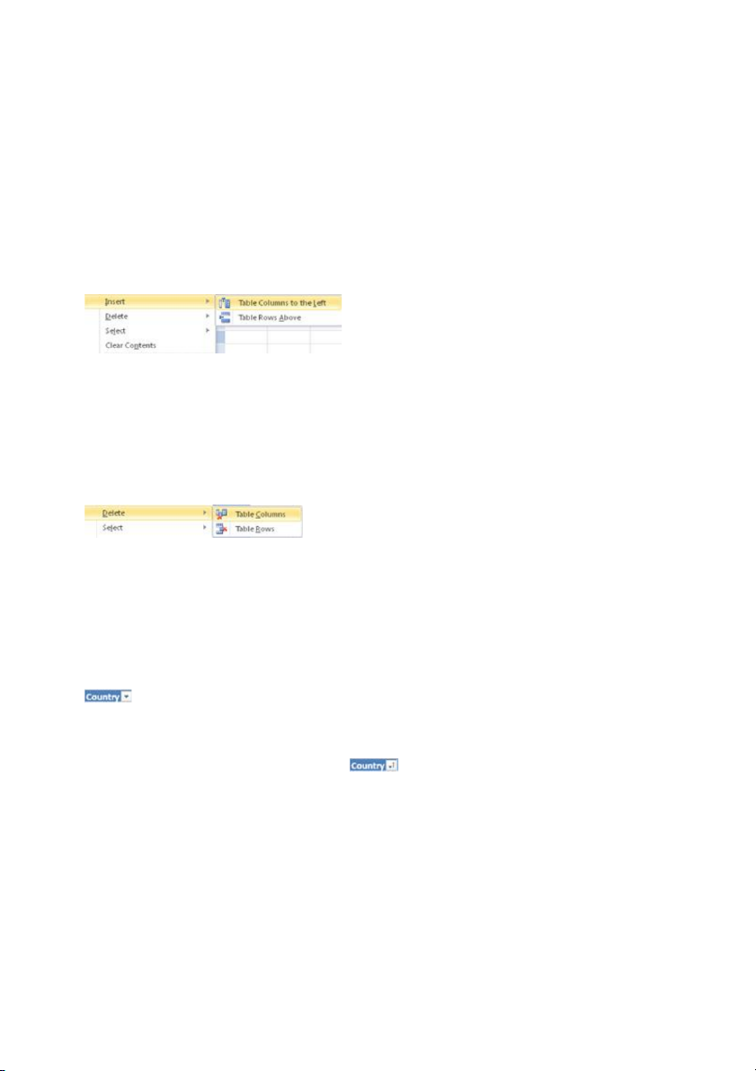
On the shortcut menu, point to Insert, and then click Table Columns to the Left.
A new column is added to the table interior. 5.
Click in cell C9, right-click, point to Insert, and then click Table Rows Above.
A new row is added to the table. 6.
Now you’ll delete a column and a row. Right-click in cell C2. 7.
Point to Delete, and then click Table Columns. The column is deleted. 8.
Click in cell C9, right-click, point to Delete, and then click Table Rows. The row is deleted.
Exercise 4: Sort a table 1.
Click the drop-down arrow on column A, the Country column. 2.
Click Sort A to Z, to sort in ascending order.
The column is sorted with Canada first, followed by the USA. The drop-down arrow now
displays a small upwards pointing arrow
to let you know that the column has been sorted. 3.
Click the drop-down arrow on Column B, the Salesperson column. 4.
Click Sort Z to A, to sort in descending order. Now you see rows and rows for
Suyama, followed by Peacock (which you can see if you scroll down the page). 5.
Click the drop-down arrow on column E, the Order ID column. 6.
Click Sort Largest to Smallest. Notice that the sort arrow moves to column E,
and that the other columns are sorted according to the sort on column E.
Exercise 5: Filter a table 1.
At the bottom of the page, click the Northwind tab. 2.
In column D, the Product Name column, click the drop-down arrow. 3.
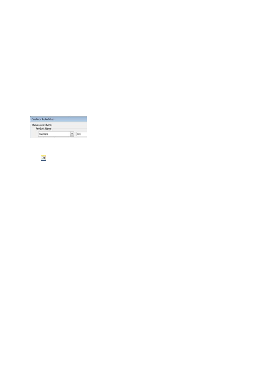
Point to Text Filters, and then click Contains. 4.
In the box to the right of “contains,” type mix to see how many products contain the text “mix.” 5. Click OK.
There are three products with the text “mix” in their titles. Notice that there’s a filter icon
on the drop-down arrow in the Product Name column, to let you know that the column is filtered. 6.
Click the drop-down arrow again in the Product Name column, and then click
Clear Filter From “Product Name.”
Now all the data is displayed again. 7.
In Column M (the Category column), click the drop-down arrow. 8.
Click in the (Select All) check box to clear the box. 9.
Click in the Canned Fruit & Vegetables box to select it, and then click . OK
Now only the canned fruit and vegetable products are visible. 10.
In column J, the Quantity Per Unit column, click the drop-down arrow. 11.
Click in the (Select All) box to clear it. 12.
Click in the 14.5 oz box to select it. Then click OK.
In column D (the Product Name column) you see the products that are 14.5 oz in the
Canned Fruit & Vegetable category. There’s a filter icon on the drop-down arrows in both column J and in column M. 13.
Clear the filters. Click the arrow in column J, and then click Clear Filter From
“Quantity Per Unit.” 14.
Next, in column M, click the drop-down arrow and then click Clear Filter From “Category.”
Now all the data is visible in the spreadsheet.
Exercise 6: Create an auto fill formula
In this exercise, you’ll figure out the commission for each order amount. 1.
At the bottom of the page, click the Formulas tab. 2.
Click in cell F2. Type an equal (=) sign, followed by an opening square bracket [. 3.
In the drop-down list that appears, double-click Order Amount. 4.
Type an ending square bracket ]. 5.
Type an asterisk (*), and then type .03.
Your formula should look like this: =[Order Amount]*.03 6. Press ENTER.
The formula automatically fills down the entire column.
Exercise 7: Add a total row 1.
Click inside the table. If necessary, click the Table Tools Design tab to reveal
the commands to work with tables. 2.
In the Table Style Options group, select the check box for Total Row. 3.
Notice that Excel automatically summed the amount in column F, the Comm
column. Excel will always sum up the right-most column if the column contains numbers.
If you don’t want the sum, click in the cell with the total, click the drop-down arrow, and then click None. 4.
Click in the total row in column C, the Order Amount column. 5.
Click the drop-down arrow, and then click Sum.
Excel totals the column: $1,228,327.40.
Exercise 8: (Optional) Add the Order Amount and the Commissions
In this exercise, you’ll add together the Order Amounts and the Commission amounts. 1.
Click in cell C804 (three rows down from the total in column C). 2.
Type an equal sign (=), and then type SUM, followed by an opening parenthesis (. 3.
Type the table name: Table2. 4.
Type an opening square bracket [.
A list of all the column names appears. 5.
Double-click Order Amount to get the column name into the formula. 6.
Type a closing square bracket ] followed by a comma (,). 7.
Type the table name: Table2.
Typing the table name again when you’re writing a formula outside the table allows you
to get the list of column names again when you type an opening square bracket. 8.
Type an opening square bracket [. 9.
In the list of column names, double-click Comm 10.
Type a closing square bracket ], followed by a closing parenthesis ). 11.
Your formula should look like this: =SUM(Table2[Order Amount],Table2[Comm]). 12. Press ENTER. 13.
The result is 1265177.222 (the numbers after the decimal point will depend on
how the decimal formatting in your version of Excel is set up). To continue the course
When you have completed the practice, click Return to course to continue.