Experiment report 2 measurement of the magnetic field inside a solenoid with finite length môn Vật lý đại cương 2 | Học viện Công Nghệ Bưu Chính Viễn Thông

Experiment Report 2
MEASUREMENT OF THE MAGNETIC FIELD INSIDE A SOLENOID
WITH FINITE LENGTH
Verification of the instructors Name: Hồ Sỹ Hoàng Anh Class: ICT-02 Student ID: 202417092 Group: 1 I. Experiment Motivations
-Study the magnetic field in a real solenoid and compare the obtained results with the
theoretical ones based on Bio-Savart’s law.
-Investigate the magnetic field at a position along the axis of solenoid
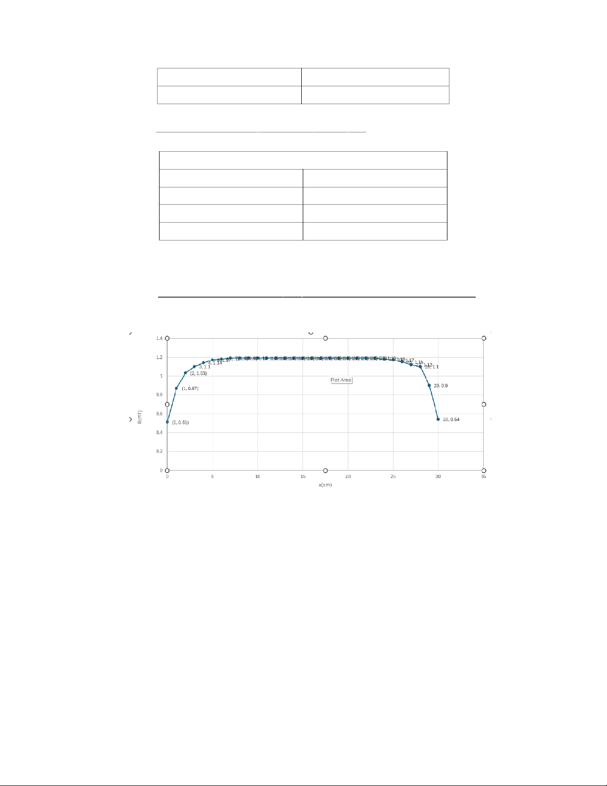
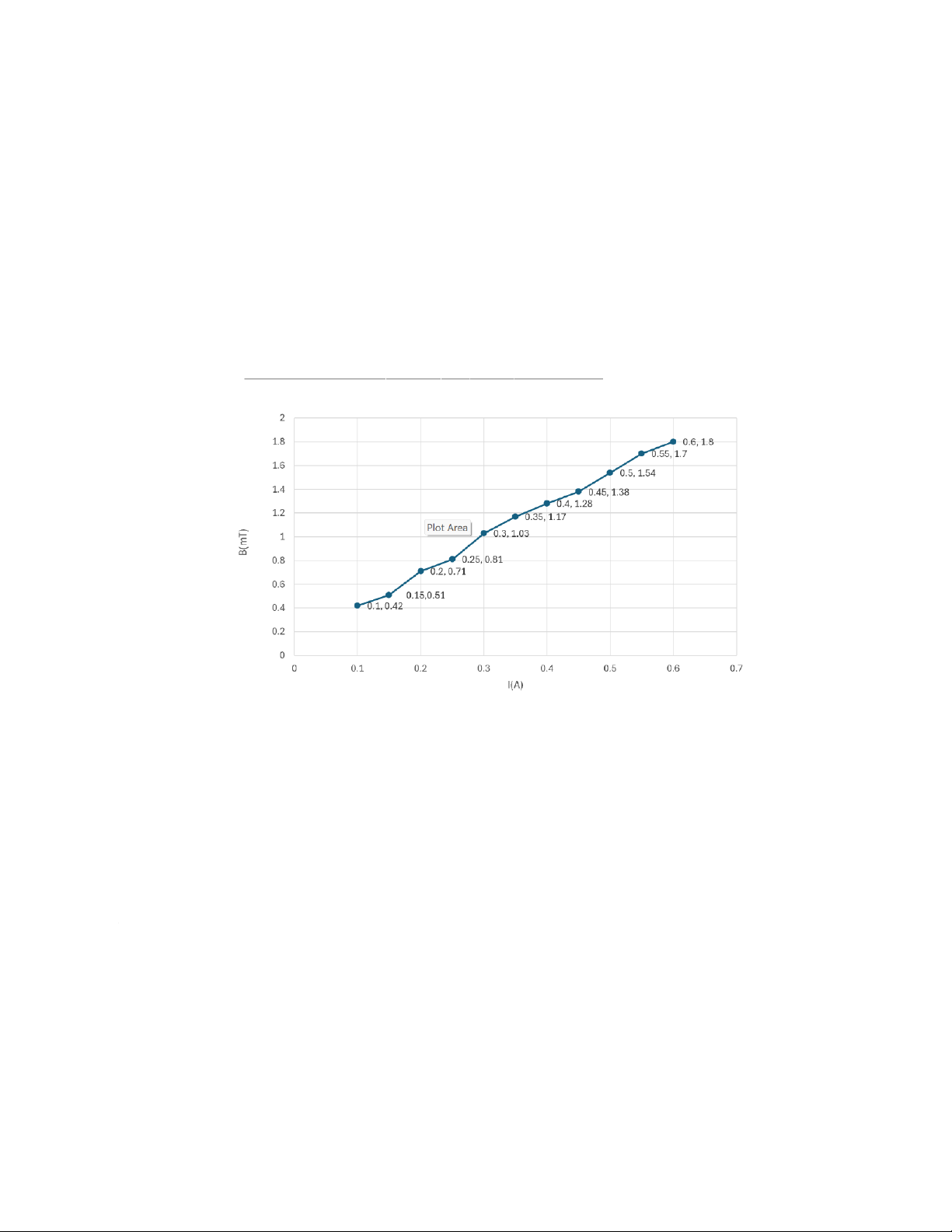
-Investigate the relationship between the magnetic field and the current through the solenoid II. Experimental Result 1. Investigation of the magnetic field at the posit ion along – the B( axis x) of solenoid I = 0.3 (A) x (cm) B (mT) x (cm) B (mT) x (cm) B (mT) 0 0.51 10 1.19 20 1.19 1 0.87 11 1.19 21 1.19 2 1.03 12 1.19 22 1.19 3 1.10 13 1.19 23 1.19 4 1.14 14 1.19 24 1.18 5 1.17 15 1.19 25 1.17 6 1.18 16 1.19 26 1.15 7 1.19 17 1.19 27 1.12 8 1.19 18 1.19 28 1.10 9 1.19 19 1.19 29 0.90 30 0.54 2. Measurement of the relationship between the magnetic field and the curre solenoid – B(I) x = 15 (cm) I (A) B (mT) 0.10 0.42 0.15 0.51 0.20 0.71 0.25 0.81 0.30 1.03 0.35 1.17 0.40 1.28 0.45 1.38 0.50 1.54 0.55 1.70 0.60 1.80 3. Comparison of experimental and theoretical magnetic fi eld I = 0.4 (A) x (cm) B (mT) 0 0.765 15 1.862 30 0.798 III. Data Analysis 1. Relationship between the magnetic field and the position of the probe ins Comment:
-The graph demonstrates that the magnetic field inside a solenoid depends on the position of the probe inside.
-The magnitude of the magnetic field increases from x = 0 cm to x = 7 cm, and then it stabe until x = 23 cm.
-Especially, the uniform magnetic field appears from x = 7 cm to x = 23cm
-After x = 23 cm until x = 30 cm, the magnitude decreases from 1.18 mT to 0.54 mT.
-According to the graph, we can see that the graph is symmetric around the x = 15 cm. 2. Relationship between the magnetic field and the applied vol tage Comment:
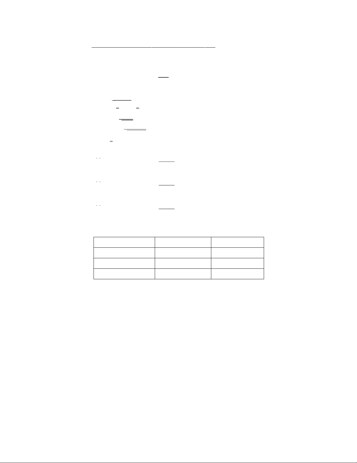
-The graph illustrates that the magnitude of the magnetic field and the current has a linear relationship. 3. Comparison of experimental and theoretical magnetic fi eld We have: 𝜇0𝜇𝑟
𝐵 = 2. 𝐼. 𝑛0(𝑐𝑜𝑠𝛾1 − 𝑐𝑜𝑠𝛾 )2 In this case, 𝜇𝑟 = 1
𝑛 = 𝑁 =750 = 2500 (turns/m) 0𝐿 300×10 −3 𝐼0 = 𝐼√2 = √ 0.4 2 = 0.566 (A)
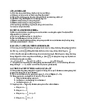
𝑐𝑜𝑠𝛾1= 𝑥√𝑅2+𝑥2
𝑐𝑜𝑠𝛾2= −𝐿−𝑥 √𝑅2+(𝐿−𝑥)2 𝑅 = 𝐷 = 0.020 (𝑚) 2
a) 𝑥 = 0 (𝑐𝑚): 𝑐𝑜𝑠𝛾 1 = 0, 𝑐𝑜𝑠𝛾 2 = −0.998 −7
𝐵 = 𝜇0𝜇𝑟 𝐼𝑛 (𝑐𝑜𝑠 𝛾 − 𝑐𝑜𝑠 𝛾
) = 4𝜋×10 × 0.566 × 2500 × (0 + 0.998) = 0.887 (𝑚𝑇) 20 1 2 2
b) 𝑥 = 15 (𝑐𝑚): 𝑐𝑜𝑠𝛾 1 = 0.991, 𝑐𝑜𝑠𝛾 2 = −0.991 −7
𝐵 = 𝜇0𝜇𝑟 𝐼𝑛 (𝑐𝑜𝑠 𝛾 − 𝑐𝑜𝑠 𝛾
) = 4𝜋×10 × 0.566 × 2500 × 2 × 0.991 = 1.762 (𝑚𝑇) 20 1 2 2
c) 𝑥 = 30(𝑐𝑚): 𝑐𝑜𝑠𝛾 1 = 0.998, 𝑐𝑜𝑠𝛾 2 = 0 −7
𝐵 = 𝜇0𝜇𝑟 𝐼𝑛 (𝑐𝑜𝑠 𝛾 − 𝑐𝑜𝑠 𝛾
) = 4𝜋×10 × 0.566 × 2500 × (0.998 − 0) = 0.887 (𝑚𝑇) 20 1 2 2
Comparison between theoretical values and experimental values: x (cm)
Btheoretical (mT) Bexperimental (mT) 0 0.887 0.765 15 1.762 1.826 30 0.887 0.798
Compare with the obtained result in the experiment:
-The result from the experiment is approximately close to the theoretical values.
-The value at x = 15 cm is the same, but at x = 0 cm and 30 cm, the difference
between theoretical values and experimental ones is more than 10%.
-The difference is due to the uncertainty of the instruments used.