Homework 3 Môn Inventory Management | Trường Đại học Quốc tế, Đại học Quốc gia Thành phố Hồ Chí Minh

lOMoAR cPSD| 58605085
School of Industrial Engineering & Management (IEM) Inventory Management
International University, VNU-HCM
Instructor: Dr. Nguyen Van Hop
TRAN PHAN NHAT KHUE – IELSIU19033 Homework 3_Chapter 3
Deadline: Class Day next week I.
Problem statement: Lot sizing for individual items when demand is time-varying
- Assumption: Known but varying demand (predetermined pattern) given economic data (holding, setup, unit variable cost,…), demand pattern.
- Decision variable: Optimal order schedule (order at which period and the order quantities)
- Method: Heuristics method (Silver-Meal, Periodic Order Quantity, Least Unit cost method, Part period balancing, L4L) and Dynamic
programming method (Wagner-Whitin) or basic EOQ (Fixed order quantity) lOMoAR cPSD| 58605085 II. Homework:
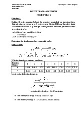
Problem 1: (6.2/224 Silver et.al. (1998) Book)
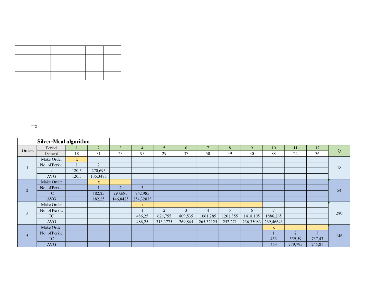
The demand pattern for another type of filter is: Jan. Feb. Mar. Apr. May June 18 31 23 95 29 37 July Aug. Sept. Oct. Nov. Dec. 50 39 30 88 22 36
Those filters cost the company $4.75 each; ordering and carrying costs are $35 and 0.24 $/$/year respectively. The variability coefficient equals 0.33.
Use the Silver – Meal heuristics to determine the sizes and timing of replenishments of stock.
Variability coefficient: A parameter to determine when to use heuristics method, when demand pattern having variability exceeds some threshold
value, it makes sense to change to a heuristic. It is Variability coefficient (VC). In particular, if VC <0.2, Use simple EOQ. Otherwise, Use heuristic. σD VC= . D
From the table, we can see that the company should order in: - Period 1 with Q = 18 - Period 2 with Q = 54 lOMoAR cPSD| 58605085 - Period 4 with Q = 280 - Period 10 with Q = 16 lOMoAR cPSD| 58605085
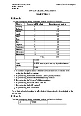
Problem 2: (6.10/224 Silver et.al. (1998) Book)
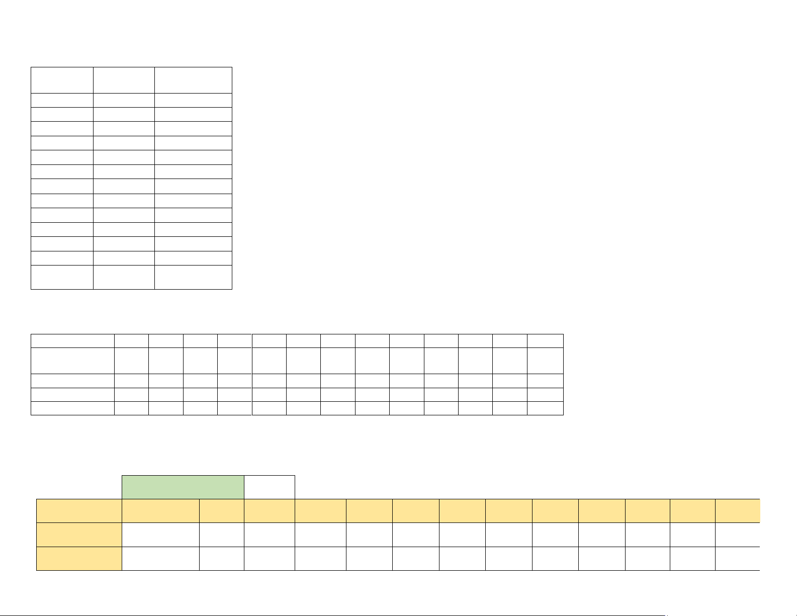
Consider a company facing a demand pattern and costs as follows: Month Sequential Requirements number (units) January 1 20 February 2 40 March 3 110 April 4 120 May 5 60 June 6 30 July 7 20 August 8 30 September 9 80 October 10 120 November 11 130 December 12 40 Total 800
Given: Fixed ordering cost A = $25.00, carrying cost r (per month) = $0.05 (Carrying costs are very high in this industry) and unit variable cost v = $4.00.
Using a “three-month” decision rule, the replenishment schedule and associated costs are as follows: Month 1 2 3 4 5 6 7 8 9 10 11 12 Total Starting 0 150 110 0 90 30 0 110 80 0 170 40 inventory Replenishment 170 0 0 210 0 0 130 0 0 290 0 0 800 Requirements 20 40 110 120 60 30 20 30 80 120 130 40 800 Ending inventory 150 110 0 90 30 0 110 80 0 170 40 0 780
Total replenishment costs: $110.00 Total carrying costs: $156.00
Total replenishment + carrying: $256.00
a/ Construct a replenishment schedule and calculate the associated costs using the Fixed Economic Order Quantity method. a. EOQ 130 Month 1 2 3 4 5 6 7 8 9 10 11 12 Total Starting Inventory 0 110 70 90 100 40 10 120 90 10 20 20 Replenishment 130 130 130 130 130 130 20 800 lOMoAR cPSD| 58605085 Requirements 20 40 110 120 60 30 20 30 80 120 130 40 800 Ending Inventory 110 70 90 100 40 10 120 90 10 20 20 0 680
Total replenishment costs 175 Total carrying costs 136 Total costs 311
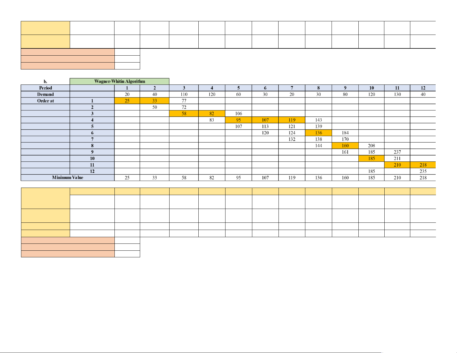
b/ Repeat using the Wagner-Whitin algorithm. Month 1 2 3 4 5 6 7 8 9 10 11 12 Total Starting Inventory 0 40 0 120 0 50 20 0 0 0 170 40 Replenishment 60 230 110 30 80 290 800 Requirements 20 40 110 120 60 30 20 30 80 120 130 40 800 Ending Inventory 40 0 120 0 50 20 0 0 0 170 40 0 440
Total replenishment costs 150 Total carrying costs 88 Total costs 238
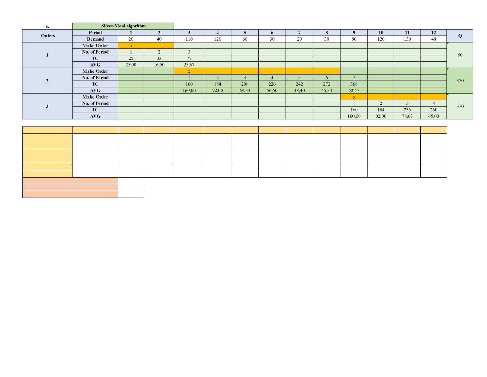
c/ Repeat using the Silver – Meal heuristic. lOMoAR cPSD| 58605085 Month 1 2 3 4 5 6 7 8 9 10 11 12 Total Starting Inventory 0 40 0 260 140 80 50 30 0 290 170 40 Replenishment 60 370 370 800 Requirements 20 40 110 120 60 30 20 30 80 120 130 40 800 Ending Inventory 40 0 260 140 80 50 30 0 290 170 40 0 1100
Total replenishment costs 75 Total carrying costs 220 Total costs 295
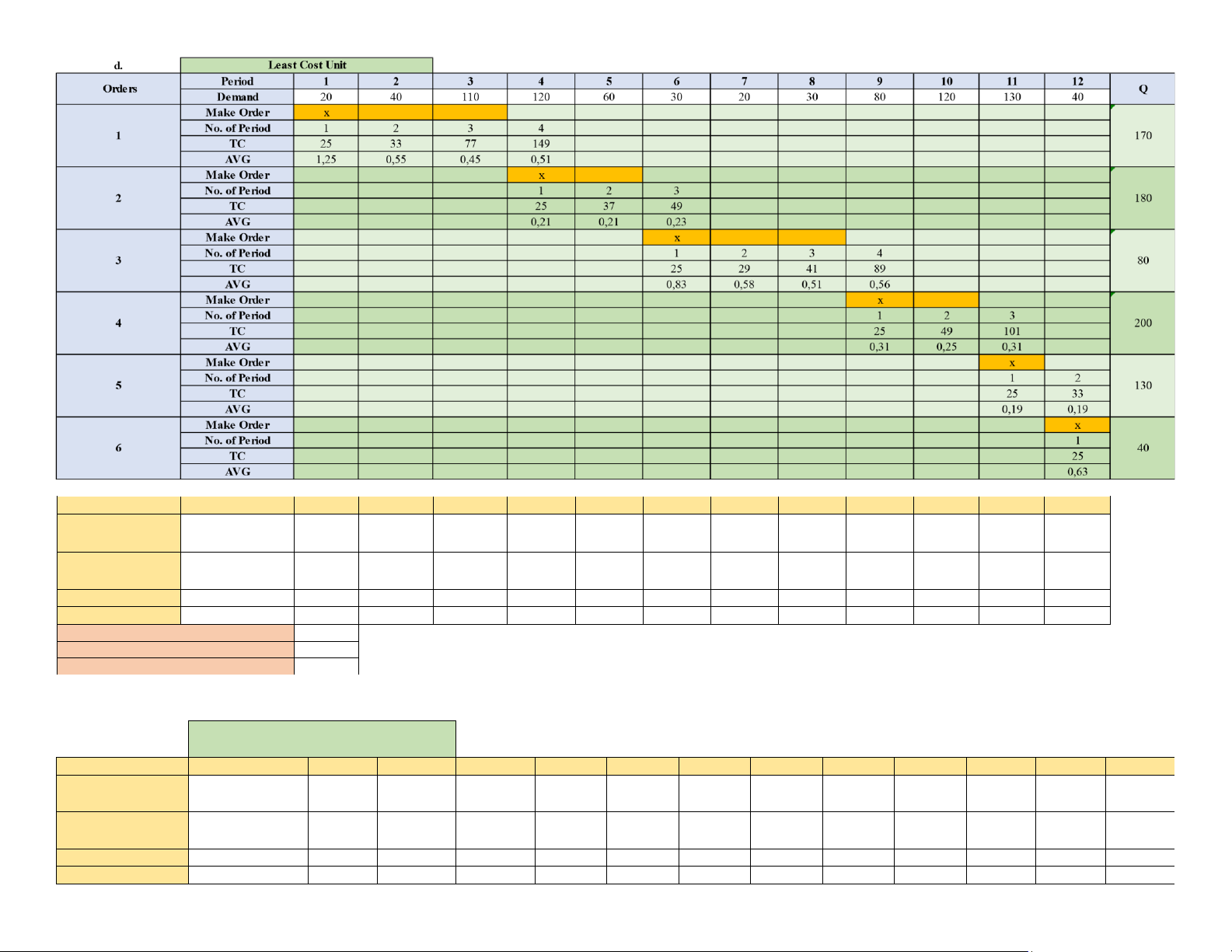
d/ Repeat using the Least Unit cost method lOMoAR cPSD| 58605085 Month 1 2 3 4 5 6 7 8 9 10 11 12 Total Starting Inventory 0 150 110 0 60 0 50 30 0 120 0 0 Replenishment 170 180 80 200 130 40 800 Requirements 20 40 110 120 60 30 20 30 80 120 130 40 800 Ending Inventory 150 110 0 60 0 50 30 0 120 0 0 0 520
Total replenishment costs 150 Total carrying costs 104 Total costs 254 .
e/ Repeat using the Part-period balancing method. e.
Part-period balancing method. Month 1 2 3 4 5 6 7 8 9 10 11 12 Total Starting Inventory 0 40 0 120 0 80 50 30 0 120 0 40 Replenishment 60 230 140 0 200 0 170 800 Requirements 20 40 110 120 60 30 20 30 80 120 130 40 800 Ending Inventory 40 0 120 0 80 50 30 0 120 0 40 0 480 lOMoAR cPSD| 58605085
Total replenishment costs 125 Total carrying costs 96 Total costs 221
f/ Repeat using the Periodic Ordering Quantity method. f.
Periodic Ordering Quantity method. Average Demand D-bar 67 Replenishment T 2 Cycle Month 1 2 3 4 5 6 7 8 9 10 11 12 Total Starting Inventory 0 40 0 120 0 30 0 30 0 120 0 40 Replenishment 60 230 90 50 200 170 800 Requirements 20 40 110 120 60 30 20 30 80 120 130 40 800 Ending Inventory 40 0 120 0 30 0 30 0 120 0 40 0 380
Total replenishment costs 150 Total carrying costs 76 Total costs 226
Problem 3: (6.17/224 Silver et.al. (1998) Book)
Consider a company facing a demand pattern and costs as follows: Month
Sequential number Requirements (units) January 1 350 February 2 200 March 3 0 April 4 150 May 5 500 June 6 600 July 7 450 August 8 350 September 9 200 October 10 0 November 11 150 December 12 200 Total 3150
Given the fixed ordering cost A = $50, carrying cost r (per month) $1.05, unit variable cost v = $65.00/ unit.
a/ Construct a replenishment schedule and calculate the associated costs using the Fixed Economic Order Quantity method. lOMoAR cPSD| 58605085 a. EOQ 630 Month 1 2 3 4 5 6 7 8 9 10 11 12 Total Starting Inventory 0 280 80 80 560 60 90 270 550 350 350 200 Replenishment 630 630 630 630 630 3150 Requirements 350 200 0 150 500 600 450 350 200 0 150 200 3150 Ending Inventory 280 80 80 560 60 90 270 550 350 350 200 0 2870
Total replenishment costs 1250 Total carrying costs 195877,5 Total costs 197127,5
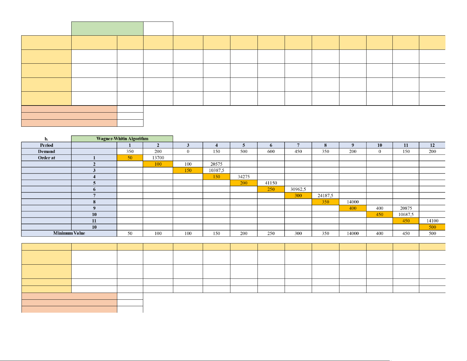
b/ Repeat using the Wagner – Whitin algorithm. Month 1 2 3 4 5 6 7 8 9 10 11 12 Total Starting Inventory 0 0 0 0 0 0 0 0 0 0 0 0 Replenishment 350 200 150 500 600 450 350 200 150 200 3150 Requirements 350 200 0 150 500 600 450 350 200 0 150 200 3150 Ending Inventory 0 0 0 0 0 0 0 0 0 0 0 0 0
Total replenishment costs 500 Total carrying costs 0 Total costs 500
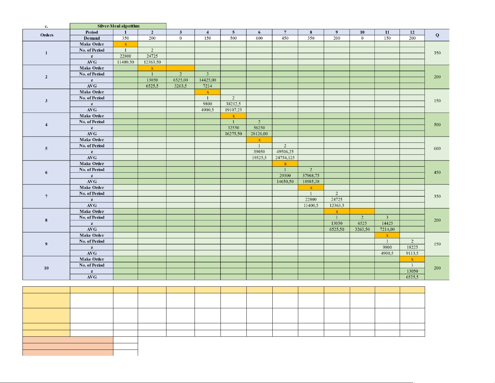
c/ Repeat using the Silver – Meal heuristic. lOMoAR cPSD| 58605085 Month 1 2 3 4 5 6 7 8 9 10 11 12 Total Starting Inventory 0 0 0 0 0 0 0 0 0 0 0 0 Replenishment 350 200 150 500 600 450 350 200 150 200 3150 Requirements 350 200 0 150 500 600 450 350 200 0 150 200 3150 Ending Inventory 0 0 0 0 0 0 0 0 0 0 0 0 0
Total replenishment costs 500 Total carrying costs 0 Total costs 500 lOMoAR cPSD| 58605085
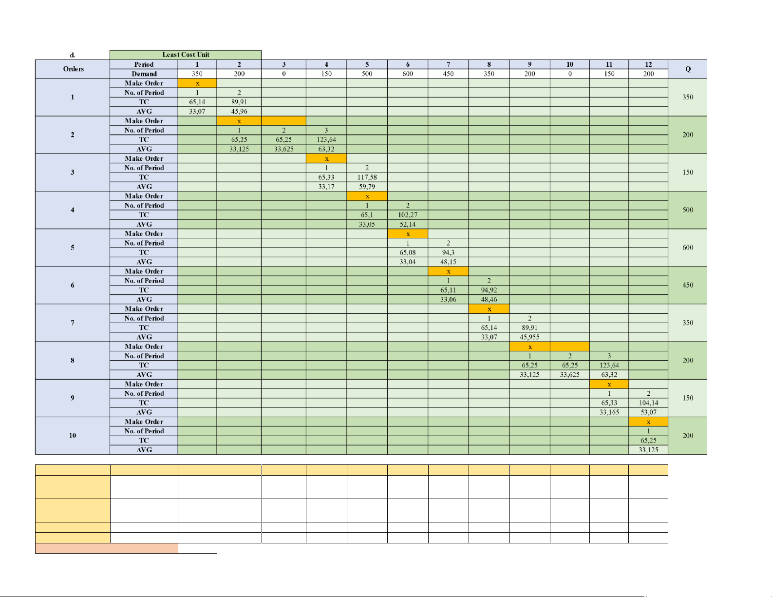
d/ Repeat using the Least Unit Cost method. Month 1 2 3 4 5 6 7 8 9 10 11 12 Total Starting Inventory 0 0 0 0 0 0 0 0 0 0 0 0 Replenishment 350 200 150 500 600 450 350 200 150 200 3150 Requirements 350 200 0 150 500 600 450 350 200 0 150 200 3150 Ending Inventory 0 0 0 0 0 0 0 0 0 0 0 0 0
Total replenishment costs 500 lOMoAR cPSD| 58605085 Total carrying costs 0 Total costs 500
e/ Repeat using the Part – period Balancing method. e.
Part-period balancing me thod. Month 1 2 3 4 5 6 7 8 9 10 11 12 Total Starting Inventory 0 0 0 0 0 0 0 0 0 0 0 0 Replenishment 350 200 0 150 500 600 450 350 200 0 150 200 3150 Requirements 350 200 0 150 500 600 450 350 200 0 150 200 3150 Ending Inventory 0 0 0 0 0 0 0 0 0 0 0 0 0
Total replenishment costs 500 Total carrying costs 0 Total costs 500
f/ Repeat using the Period Ordering Quantity method. f.
Periodic Ordering Quantity method. Average Demand D-bar 263 Replenishment T 1 Cycle Month 1 2 3 4 5 6 7 8 9 10 11 12 Total Starting Inventory 0 0 0 0 0 0 0 0 0 0 0 0 Replenishment 350 200 0 150 500 600 450 350 200 0 150 200 3150 Requirements 350 200 0 150 500 600 450 350 200 0 150 200 3150 Ending Inventory 0 0 0 0 0 0 0 0 0 0 0 0 0
Total replenishment costs 500 Total carrying costs 0 Total costs 500 Problem 4:
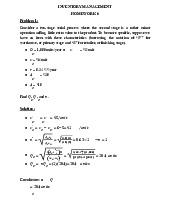
A component used in a manufacturing facility is ordered from an outside supplier.
The component is used in a variety of finished items and therefore the demand is high.
Forecast demand (in thousands) over the next 8 weeks is: Week 1 2 3 4 5 Demand 21 33 29 15 9
Each component costs 70 cents and the inventory carrying charge rate is 0.56 cents
($0.0056) per unit per week. The fixed order cost is $300. Assume instantaneous delivery.
What is the ordering policy recommended by DP algorithm? z*1 = 0
c1,2 = 300 + 0.7*21 = 314.7 z*2 = z*1 + c1,2 = 314.7 = 314.7 p*2 = 1 lOMoAR cPSD| 58605085
c1,3 = 300 + 0.7*(21+33) + 0.00392*33 = 337.93 c2,3
= 300 + 0.7*33 = 323.1 z*3 = min (337.92, 323.1 + 314.) = 337.92 p*3 = 1
c1,4 = 300 + 0.7*(21+33+29) + 0.00392*(33+29*2) = 358.457 c2,4 =
343.513 c3,4 = 320.3 z*4 = min (358.457, 314.7 + 343.513, 337.92 + 320.3) = 358.457 p*4 = 1
c1,5 = 300 + 0.7*(21+33+29+15) + 0.00392*(33+29*2+ 15*3) = 369.13
c2.5 = 354,13 c3.5 = 330.86 c4,5 = 310.5 z*5 = min (369.13, 668.83,
668.72, 669.957) = 369.13 p*5 = 1
c1,6 = 375.57 c2,6 = 360.54 c3,6 = 337.23 c4,6 = 316.84 c5,6 = 306.3 z*6 =
min (375.57, 675.24, 675.15, 675.3, 375.43) = 375.57 p*6 = 1
Therefore, by DP algorithm, we should make an order from week 1 with Q = 107.