iêu đề chi tiết rõ ràng (30 ký tự) sẽ được duyệt nhanh hơn Bao gồm Trườnglớp môn học chươngb
abc
Môn: Kiểm toán tài chính 160 tài liệu
Trường: Trường Đại học Kinh Tế Quốc Dân 8.6 K tài liệu
Tác giả:


Preview text:
Article
Path Planning and Motion Control of Robot Dog Through Rough
Terrain Based on Vision Navigation
Tianxiang Chen * , Yipeng Huangfu *,† , Sutthiphong Srigrarom * and Boo Cheong Khoo
Mechanical Engineering, National University of Singapore, Singapore 117576, Singapore; mpekbc@nus.edu.sg
* Correspondences: e1373675@u.nus.edu (T.C.); hfyp@ucla.edu (Y.H.); spot.srigrarom@nus.edu.sg (S.S.)
† Current address: Mechanical and Aerospace Engineering, University of California Los Angeles, Los Angeles, CA 90095, USA
Abstract: This article delineates the enhancement of an autonomous navigation and obstacle avoid-
ance system for a quadruped robot dog. Part one of this paper presents the integration of a so-
phisticated multi-level dynamic control framework, utilizing Model Predictive Control (MPC) and
Whole-Body Control (WBC) from MIT Cheetah. The system employs an Intel RealSense D435i depth
camera for depth vision-based navigation, which enables high-fidelity 3D environmental mapping
and real-time path planning. A significant innovation is the customization of the EGO-Planner to
optimize trajectory planning in dynamically changing terrains, coupled with the implementation of a
multi-body dynamics model that significantly improves the robot’s stability and maneuverability
across various surfaces. The experimental results show that the RGB-D system exhibits superior
velocity stability and trajectory accuracy to the SLAM system, with a 20% reduction in the cumulative
velocity error and a 10% improvement in path tracking precision. The experimental results also show
that the RGB-D system achieves smoother navigation, requiring 15% fewer iterations for path plan-
ning, and a 30% faster success rate recovery in challenging environments. The successful application
of these technologies in simulated urban disaster scenarios suggests promising future applications in
emergency response and complex urban environments. Part two of this paper presents the devel-
opment of a robust path planning algorithm for a robot dog on a rough terrain based on attached
binocular vision navigation. We use a commercial-of-the-shelf (COTS) robot dog. An optical CCD
Citation: Chen, T.; Huangfu, Y.;
binocular vision dynamic tracking system is used to provide environment information. Likewise, Srigrarom, S.; Khoo, B.C. Path
the pose and posture of the robot dog are obtained from the robot’s own sensors, and a kinematics Planning and Motion Control of
model is established. Then, a binocular vision tracking method is developed to determine the optimal
Robot Dog Through Rough Terrain
path, provide a proposal (commands to actuators) of the position and posture of the bionic robot,
Based on Vision Navigation. Sensors
and achieve stable motion on tough terrains. The terrain is assumed to be a gentle uneven terrain
2024, 24, 7306. https://doi.org/
to begin with and subsequently proceeds to a more rough surface. This work consists of four steps: 10.3390/s24227306
(1) pose and position data are acquired from the robot dog’s own inertial sensors, (2) terrain and
Academic Editors: Charalampos P.
environment information is input from onboard cameras, (3) information is fused (integrated), and
Bechlioulis and George C. Karras
(4) path planning and motion control proposals are made. Ultimately, this work provides a robust Received: 19 September 2024
framework for future developments in the vision-based navigation and control of quadruped robots, Revised: 24 October 2024
offering potential solutions for navigating complex and dynamic terrains. Accepted: 4 November 2024 Published: 15 November 2024
Keywords: quadruped robot dog; model predictive control; whole-body control; multi-level trajectory
planner; path planning; depth vision-based navigation; map generation; rough terrain; SLAM
Copyright: © 2024 by the authors.
Licensee MDPI, Basel, Switzerland. 1. Introduction
This article is an open access article
distributed under the terms and
Quadruped robots have gained significant attention in recent years due to their adapt-
conditions of the Creative Commons
ability and scalability in various environments, such as those in industrial, military, and
Attribution (CC BY) license (https://
disaster relief operations. Unlike wheeled robots, quadruped robots can easily navigate
creativecommons.org/licenses/by/
stairs and low obstacles, making them ideal for rugged terrains and densely forested areas, 4.0/).
where wheeled robots struggle [1]. This ability to traverse complex terrains has propelled
Sensors 2024, 24, 7306. https://doi.org/10.3390/s24227306
https://www.mdpi.com/journal/sensors Sensors 2024, 24, 7306 2 of 32
quadruped robots to the forefront of modern robotics research. Researchers and developers
are currently focusing on enhancing their autonomy, load-bearing capacity, and gait effi-
ciency by integrating advanced control algorithms and artificial intelligence, enabling these
robots to execute complex tasks with greater efficiency and flexibility [2].
Despite these advancements, the current navigation and control capabilities of
quadruped robots still require significant improvements, especially in complex and dy-
namic environments. Most traditional navigation systems rely on static, predefined paths,
lacking adaptability to unforeseen obstacles and dynamic changes in terrain [3]. For
instance, path planning algorithms that are effective in static environments face signifi-
cant limitations in real-time adaptability and computational efficiency when applied to
quadruped robots navigating complex terrains [4]. Additionally, maintaining stability and
smooth operation at high speeds or during dynamic maneuvers remains a challenge [5].
For example, the MIT Cheetah robot, known for its speed and agility, struggles to maintain
balance and stability when transitioning between different terrains or executing rapid
maneuvers [6]. This instability stems from the lack of integration between high-frequency
sensor feedback and low-latency control algorithms necessary for real-time adjustments [7].
Moreover, control strategies like WBC and MPC, while robust, are computationally in-
tensive. They require precise modeling of the robot’s kinematics and dynamics, which
becomes increasingly complex at higher speeds or when encountering unexpected changes
in terrain [8]. The computational demand for real-time optimization often exceeds the
capabilities of onboard processors, leading to delayed responses that can compromise
stability and increase the risk of falls or collisions [9]. Recent studies suggest that integrat-
ing reinforcement learning techniques with traditional control strategies could enhance
real-time decision-making capabilities, but this approach has yet to be fully realized in practical applications [10].
Alongside motion control, navigation and trajectory planning present another set of
critical challenges. Traditional methods, such as grid-based and sampling-based planning
algorithms, often fail to adapt efficiently to dynamic environments due to their high compu-
tational costs and suboptimal path generation [11]. These methods typically rely on static
environment models and predefined paths, which do not account for dynamic obstacles or
varying terrain conditions. As a result, the generated trajectories may not be feasible or
safe in real-time applications, especially in environments that require frequent adjustments
and recalculations of optimal paths [12]. Furthermore, current quadruped robot systems
lack a comprehensive framework that seamlessly integrates navigation, trajectory plan-
ning, and motion control. This disjointed nature often leads to inefficiencies and conflicts
in decision-making processes [13]. For example, an optimal trajectory generated by the
navigation system may be impractical for the motion control system to execute due to its
own constraints and limitations, resulting in suboptimal performance, increased energy
consumption, and reduced operational safety [14].
To address these challenges, this paper proposes an integrated system that combines
robust navigation algorithms, efficient trajectory planning methods, and advanced motion
control strategies. The integration of these components allows for real-time adaptability and
stability, even in dynamic and unpredictable environments [15]. By leveraging multi-sensor
fusion and machine learning techniques, the proposed system optimizes the entire navi-
gation and control process for quadruped robots, providing a more reliable and efficient
solution than current methods. The primary objectives of this research are to develop a ro-
bust path planning and dynamic control framework that integrates vision-based navigation
with advanced motion control techniques for quadruped robots in complex terrains and
to validate the proposed framework through extensive simulations and real-world experi-
ments [16]. Key contributions include the development of a customized 2D EGO-Planner
for optimized trajectory planning in dynamically changing terrains, the integration of MPC
and WBC to improve stability and maneuverability, and the implementation of a multi-
sensor fusion system that combines data from depth cameras and inertial measurement
units (IMUs) to enhance environmental perception and navigation accuracy. Sensors 2024, 24, 7306 3 of 32
The remainder of this paper is organized as follows: Section 2 reviews the related
work on quadruped robot navigation and control systems. Sections 3 and 4 detail the
proposed methodology, including system architecture, trajectory planning framework, and
control algorithms. Section 5 presents the experimental setup and results, highlighting the
effectiveness of the proposed approach. Section 6 discusses the findings and summarizes
the key contributions, potential improvements, and future work. Objectives
This research focuses on enhancing quadruped robot navigation and motion control
in complex environments by integrating advanced algorithms and control systems. The
primary objective is to adapt the EGO-Planner for 2D navigation, optimizing path planning
by limiting unnecessary Z-axis movement. Additionally, this work aims to implement a
combined MPC and WBC framework to improve real-time motion planning and ensure
robust control in dynamic environments. Furthermore, the research compares different
sensor fusion systems, highlighting the advantages of vision-based navigation over LiDAR
in trajectory planning and localization, particularly in terms of reduced data requirements and cost-efficiency. 2. Literature Review 2.1. Robot Dog Platform
Recent advancements in quadruped robots, or robotic dogs, have demonstrated signif-
icant progress in their capabilities, particularly in motion control and terrain adaptability.
Notable examples include Boston Dynamics’ Spot, MIT’s Cheetah, and ETH Zurich’s
ANYmal. These platforms integrate dynamic balancing algorithms and real-time feed-
back control systems, enabling robust navigation in complex environments. For instance,
Spot utilizes stereo vision, gyros, and accelerometers to process feedback for real-time
control [17], while MIT’s Cheetah leverages precise force control and high-frequency leg
dynamics to maintain stability at high speeds [18]. ETH Zurich’s ANYmal, by contrast,
focuses on using machine learning to dynamically plan movements and adapt to varying
terrains through real-time sensor fusion, including LIDAR and vision systems [19].
The research community’s advancements are also reflected in commercial models.
Unitree Robotics’ A1 and DeepRobotics’ Jueying Lite have expanded accessibility by pro-
viding open interfaces and modular designs that support the integration of custom control
algorithms. Unitree’s A1, known for its robust mobility and adaptability, excels in indus-
trial and public safety applications by autonomously optimizing its walking strategies [20].
Meanwhile, Jueying Lite prioritizes cost-effectiveness and flexibility, making it a popular
platform for consumer and research applications [21].
2.2. Trajectory Planning Algorithms
Trajectory planning plays a pivotal role in robot navigation, ensuring that the optimal
path from a starting point to a goal is found while accounting for environmental constraints
and dynamic changes. This process is typically divided into two key components: global and local planning.
2.2.1. Existing Path and Local Planning Approaches
In robot navigation, global path planning and local trajectory planning are two essen-
tial components. Global path planning aims to calculate a feasible path from a starting point
to a goal, typically using static or existing maps. Traditional algorithms, such as A* and
its variant D* Lite, are widely used for this purpose. A* is efficient in static environments
for finding the shortest path; however, in dynamic environments with moving obstacles,
it requires frequent path recomputation, which can significantly increase computational
cost and reduce real-time performance [22]. Dynamic A* (D*) improves this by updating
only the affected portions of the path in dynamic environments, reducing computational
overhead and improving adaptability [23]. Despite these advancements, D* mainly serves Sensors 2024, 24, 7306 4 of 32
as a static path generator and is less effective in scenarios requiring real-time updates during robot motion.
However, local path planning addresses real-time environmental changes, often deal-
ing with unpredictable obstacles or dynamic conditions. The Dynamic Window Approach
(DWA) is a common method, optimizing the robot’s velocity and trajectory based on its cur-
rent state and nearby obstacles. While effective in static environments, the DWA struggles
with dynamic obstacles and often gets trapped in local minima [24]. Another approach,
the Time Elastic Band (TEB), adjusts trajectory nodes to improve path smoothness and
efficiency while considering the robot’s kinematic constraints. Although the TEB enhances
path efficiency, it faces computational challenges in highly dynamic environments, limiting
its real-time application [25]. These limitations underscore the need for more adaptive local
planners in complex and changing environments.
2.2.2. Improvements in Path and Local Trajectory Planning
This study addresses the limitations of existing global and local planning algorithms
by utilizing established methods while introducing key improvements. For global path
planning, we employ the Dynamic A* (D*) algorithm to generate an initial path. D* serves as
the foundation for static obstacle avoidance but remains a preliminary path generator [26].
The global path generated by D* acts as a general guideline for robot navigation without
any modifications to the algorithm.
The main contribution of this study lies in the local trajectory planning through the
adaptation of the EGO-Planner into a two-dimensional (2D) version, specifically optimized
for ground-based quadruped robots. Unlike traditional planners that rely on existing global
maps [27], this 2D EGO-Planner dynamically updates the trajectory using real-time sensor
feedback, allowing the robot to navigate complex, unknown environments [28].
The global path produced by D* serves as an initial rough input to the 2D EGO-
Planner, which not only acts as a dynamic path optimizer but also incorporates kinematic
constraints. The final output is a time-parameterized trajectory that includes the robot’s
positions, velocities, and accelerations over time. Specifically, at each time step t, the planner
computes the center of mass (CoM) positions p(t), velocities v(t), and accelerations a(t) as
{p(t), v(t), a(t)}, t ∈ [t0, t f ]. This planner ensures real-time adjustments based on sensory
data, improving adaptability and reducing the likelihood of the robot becoming trapped in
local minima. A more detailed explanation of this adaptation is provided in Section 4.6.
2.3. Control Systems for Quadruped Robots
Control systems for quadruped robots are typically divided into low-level controllers
and high-level planners. Low-level controllers handle joint control and stability, while
high-level planners generate motion trajectories and adapt to dynamic environments. Coor-
dination between these layers is essential for robust locomotion, especially in unpredictable
terrains. Various approaches have been proposed to address challenges in both layers,
optimizing performance across different conditions.
2.3.1. Existing Control Strategies and Limitations
Low-level strategies, like PD control, are essential for joint-level motion but are limited
in adapting to dynamic and unpredictable environments. Advanced methods, including
computed torque control and sliding mode control, have been explored but still struggle
with real-time adaptation to complex terrains. High-level methods, such as Zero-Moment
Point and inverse kinematics (IK)-based planning, are effective in specific locomotion tasks
but often lack the flexibility to adapt to dynamic, unstructured environments due to their
reliance on pre-planned motions [29].
To overcome these limitations, MPC has been widely adopted for its adaptability in
complex environments. By considering the robot’s current state and dynamic constraints,
MPC provides robust motion optimization, while Whole-Body Control (WBC) ensures the Sensors 2024, 24, 7306 5 of 32
seamless execution of planned trajectories. This approach has proven effective in real-world
applications, such as MIT’s Cheetah robot [30].
2.3.2. Implementation and Adaptation
Adapting the MPC and WBC combination to our quadruped robot required addressing
challenges related to the mechanical structure, including motor specifications and joint
torque limits. Additionally, the integration of foot-end force sensors for real-time feedback
demanded precise calibration to ensure accurate torque control. We used PD controllers at
the low level to execute the high-level commands generated by MPC and WBC, controlling
each motor’s torque and ensuring precise joint-level movement. After resolving these
hardware challenges, we successfully established a control framework, laying a foundation
for dynamic stability and future navigation experiments. 3. Dynamic Motion Control
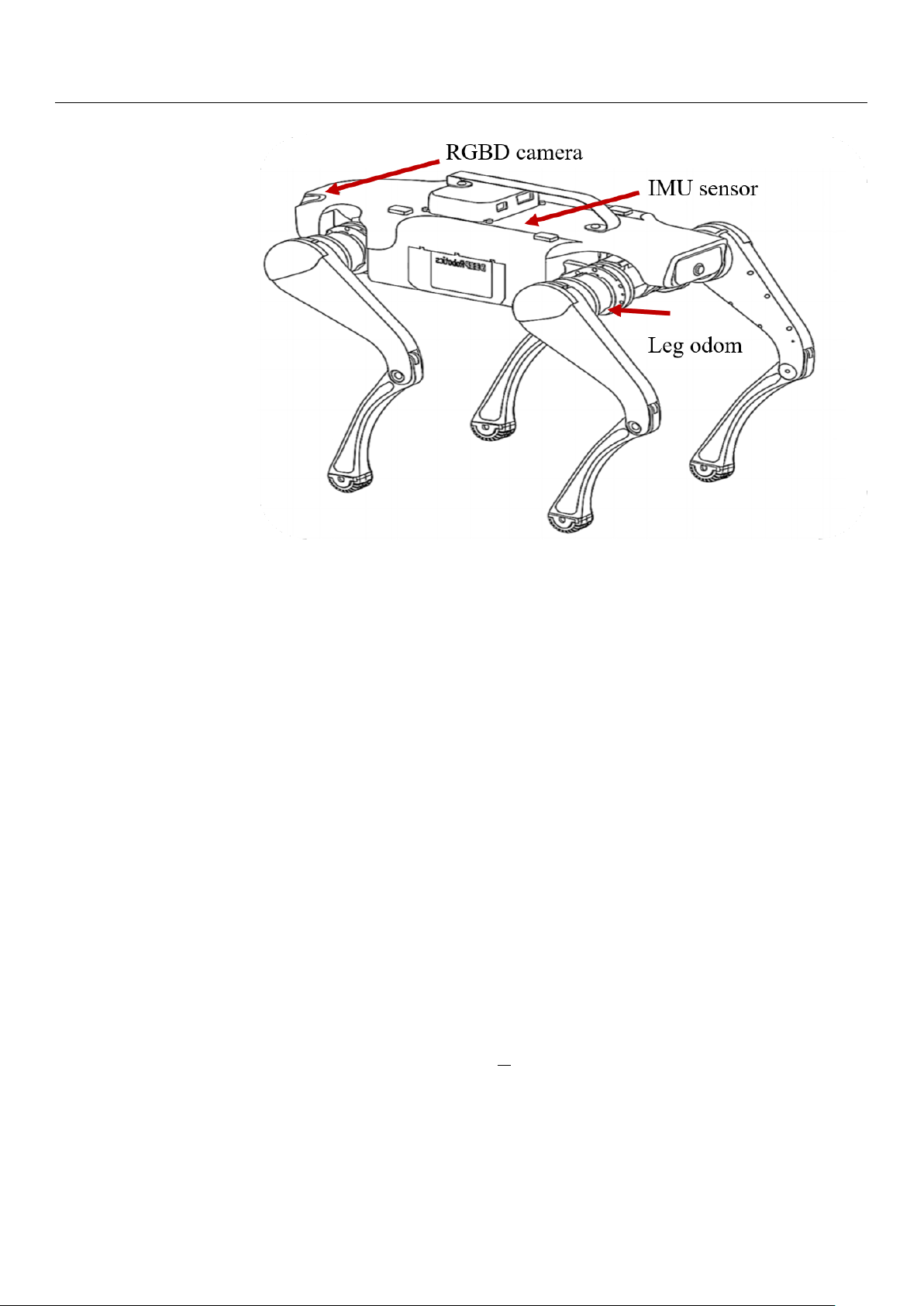
3.1. Hardware Overview of the Quadruped Robot
In this study, we built a quadruped robotic dog simulation platform based on Gazebo
and RViz, and we integrated multiple sensors, including RGB-D cameras, IMUs, and
odometers, using an Extended Kalman Filter (EKF) to improve state estimation [31]. The
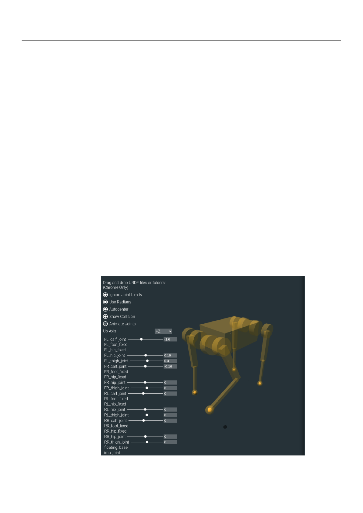
robotic dog used in our simulations is the Lite3P model developed by Unitree Robotics, as
shown in Figure 1. This robot features a simplified 12-degree-of-freedom (DOF) structure,
with each leg having three joints: a hip, a thigh, and a calf. This mechanical configuration
is sufficient to support subsequent experiments. The hardware layout of these sensors is
shown in Figure 2. The Intel RealSense D435i depth camera provides high-precision RGB-D
data, which are crucial for environmental perception. The IMU, a six-DOF sensor, collects
real-time acceleration and angular velocity data, and it is installed in the center of the
robot’s body to help estimate its posture during movement. Additionally, foot odometers
are installed at the hip joints of each leg, monitoring joint angles, movement speed, and
torque, ensuring precise control of the robot’s gait.
Figure 1. Simplified box model of the Lite3P quadruped robotic dog. Sensors 2024, 24, 7306 6 of 32
Figure 2. Internal sensor arrangement of the quadruped robotic dog.
3.2. Physics Modeling of the Quadruped Robot
To improve the performance of real-time trajectory planning and to enhance the com-
putational efficiency of the control algorithms, we employ a simplified centroidal dynamics
model. This approach has been widely utilized in humanoid and mobile robotics, where
representing the robot as a point mass at its CoM significantly reduces computational
complexity while preserving essential dynamic characteristics [32]. In our two-dimensional
EGO-Planner framework, the trajectory planner focuses solely on the robot’s CoM trajec-
tory rather than explicitly planning the motions of the individual legs, following similar
strategies applied in biped locomotion planning [33]. The discrete CoM trajectory points
generated by the planner are then fed into an MPC and WBC framework. Within this
control framework, inverse kinematics plays a critical role in translating the desired CoM
trajectory into joint-level actions. Specifically, the WBC component utilizes IK to compute
the joint angles required to achieve the target foot-end positions generated by MPC. This
process relies on the pseudo-inverse of the Jacobian matrix, ensuring precise control of each
leg while satisfying physical constraints such as joint limits and ground contact stability.
The centroidal dynamics model, which treats the robot as a single point mass, facilitates
the description of the robot’s physical behavior using simplified dynamic equations. This
approach provides an efficient framework for later predictive optimization and control.
The equations governing the dynamics of the robot’s CoM and rotational motion are
given in Equation (1) and Equation (2), respectively: ne
m ¨p = ∑ fi − cg (1) i=1 d ne
(Iω) = ∑ r dt i × fi (2) i=1
Here, m represents the total mass of the robot, ¨p is the acceleration of the CoM, and fi
is the ground reaction force acting at leg i. The rotational dynamics are described by the
angular velocity ω, with the inertia tensor I governing the rotational inertia of the robot’s
body. The meanings of these parameters follow the standard definitions commonly used in
centroidal dynamics models for humanoid and legged robots [32]. Sensors 2024, 24, 7306 7 of 32
In subsequent experiments, the centroidal model calculates the dynamic behavior
of the robot’s CoM, providing information on the position, velocity, and acceleration
of the CoM for correction by the EKF. When solving joint torques and distributing foot
contact forces in the WBC, the floating-base dynamics model and the multi-body dynamics
model are employed. The floating-base dynamics model calculates the motion state of the
CoM and its relationship with external forces [34], while the multi-body dynamics model
describes the relative motion between the robot’s limbs and torso, computing joint torques
and force distribution [35]. However, as the focus of this section is on the MPC and WBC
control processes, further details of the floating-base dynamics and multi-body dynamics
models are omitted. Readers interested in these models can refer to References [34,35].
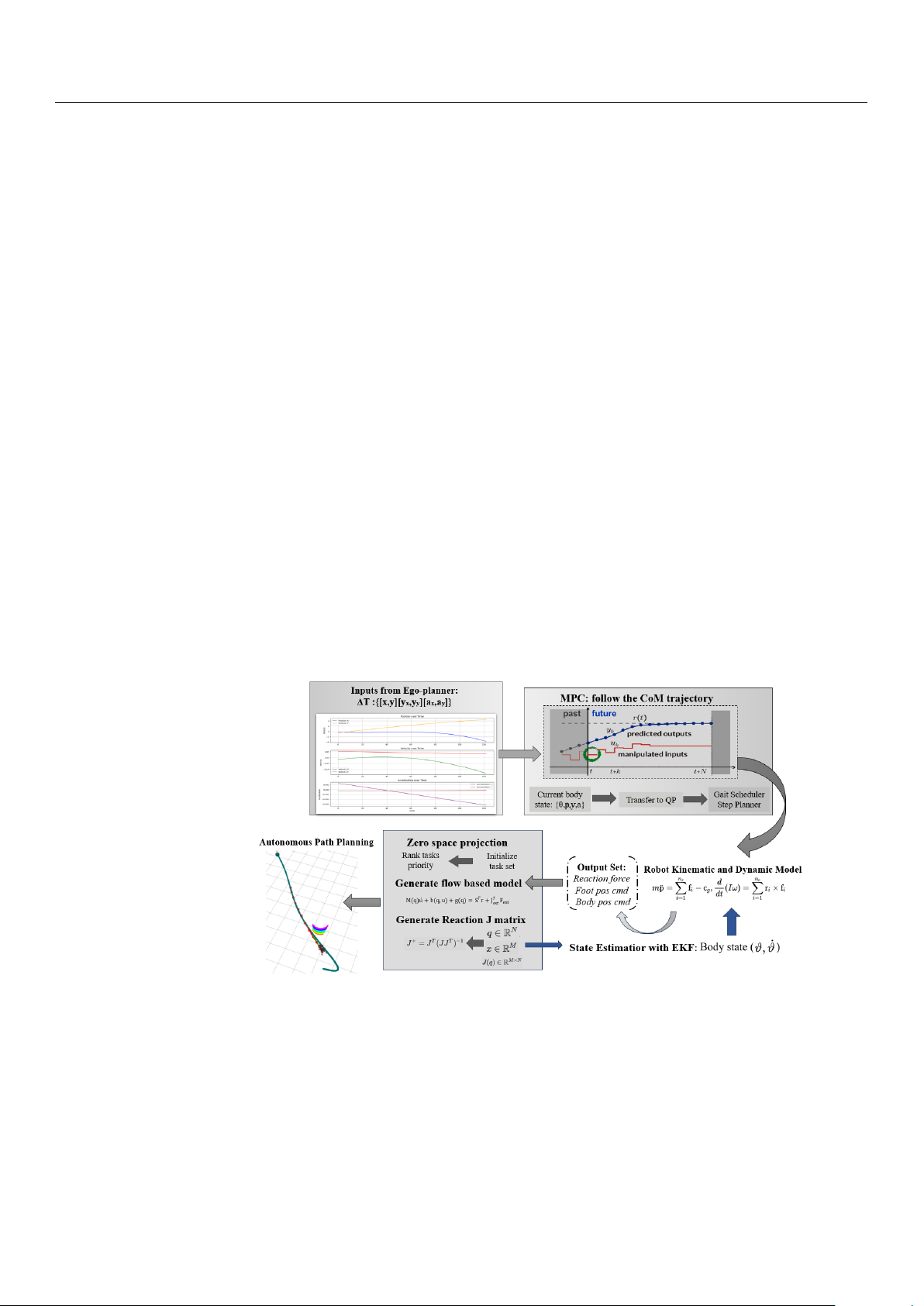
3.3. Dynamic Motion Control Model
As previously mentioned, the motion control of quadruped robots involves complex
full-body dynamics and coordination between the limbs. Consequently, motion planning
in complex terrains cannot be achieved through simple point-to-point trajectory planning.
To address this challenge, we integrated a control strategy from Cheetah with an existing
centroidal dynamics model to enable efficient motion control for quadruped robots [30].
As shown in Figure 3, once the 2D EGO-Planner generates the COM trajectory ϑt, ˙ ϑt ,
it is fed into the MPC module. Using this trajectory and the robot’s dynamic model, the
MPC calculates the desired foot positions, centroid orientation, and contact forces at each
time step. WBC then integrates these outputs to compute the contact forces and optimal
joint torques. The motors execute these control commands, incrementally guiding the
robot towards the target posture. During operation, sensors such as the IMU and foot-end
odometers provide real-time feedback, while forward kinematics calculates the actual foot
positions. An EKF fuses these data with the expected values to estimate the robot’s posture
and position. This updated state information is sent to the upper-level planner to adjust
the trajectory until the robot reaches the target.
Figure 3. Dynamic control flowchart. 3.3.1. MPC Model
The basic principles of MPC include predictive modeling, receding horizon opti-
mization, and feedback correction. During the predictive modeling phase, MPC predicts
future outputs based on current and historical inputs. Receding horizon optimization
continuously recalculates the optimal control sequence at each sampling time. Meanwhile,
feedback correction adjusts the control inputs by comparing the actual output with the
predicted output, ensuring accurate trajectory tracking. By combining the centroidal model
mentioned in Section 3.2 and relevant assumptions, we introduce the process of deriving
the system’s dynamic model for MPC. Sensors 2024, 24, 7306 8 of 32
Based on this formulation, the discrete dynamic representation of the system is ex-
pressed in Equation (3) as follows: x(k + 1) = A ˆ k x(k) + Bk f (k) + ˆ g, (3)
where x(k), Ak, Bk, ˆf(k), and ˆg represent the state vector, system matrices, contact forces,
and environmental forces, respectively. These parameters follow the standard definitions
widely used in MPC formulations, where x(k) consists of the position, velocity, and ori-
entation of the robot’s CoM; Ak and Bk represent the system and input matrices; and ˆf(k)
includes the contact forces acting on the robot [36].
The state vector x(k) is defined as h
x = Θ⊤, p⊤, ⊤
ω , p⊤i⊤, (4)
where Θ represents the orientation of the robot’s base, p represents the position of the
robot’s CoM, and ω refers to the angular velocity of the robot’s base.
The quadratic programming (QP) optimization problem for MPC is then posed to
minimize the deviation between the predicted state and the reference trajectory while bal-
ancing the control effort. The weight matrices Q and R, which control the trade-off between
tracking accuracy and energy efficiency, are also standard in MPC formulations [37].
Next, the system matrices Ak and Bk, which describe the time evolution of the CoM
and the impact of the contact forces, are defined in Equations (5) and (6) as follows: 1 3×3
03×3 R2(ψk)∆t 03×3 03×3 · · · 03×3 0 0 A = 3×3 13×3 03×3 13×3∆t 3×3 · · · 03×3 , B = . (5)
03×3 03×3 13×3 03×3 G−1[r1] ∆ ∆ × t · · ·
gI−1[rn]× t
03×3 03×3 03×3 13×3 13×3∆t/m · · · 13×3∆t/m
To minimize the deviation between the system’s predicted state and the reference
trajectory, the following QP optimization problem is posed in Equation (6): m
min ∑ ∥x(k + 1) − xref(k + 1)∥Q + ∥ f(k)∥R. (6) x, f k=0
This objective function seeks to reduce both the deviation from the desired trajectory
and the magnitude of the control inputs while also considering energy consumption constraints [37].
As shown in Figure 4, MPC acts as the upper-level controller, receiving geometric
information about CoM from the 2D EGO-Planner, which includes time series data of
velocity and position. The CoM position is given by x k ˙xk p p k+1 − pk k = = yk , ˙pk = ˙yk ∆ (7) T zk ˙zk
where pk represents the CoM position at time tk, and ˙pk represents the corresponding ve-
locity. Equation (7) gives the expression of the planned CoM position and the CoM velocity.
In the MPC computation process, the floating-base dynamics model is integrated to
improve accuracy in deriving the dynamic behavior of the CoM. The use of the floating-
base model allows the controller to account for the robot’s degrees of freedom, providing a
more accurate representation of CoM attitude changes; the attitude of the CoM is mainly
computed by maintaining balance. MPC computes the forces exerted by each leg on the
CoM and uses these forces to derive changes in the CoM’s attitude. The CoM acceleration
is calculated using the following equation: Sensors 2024, 24, 7306 9 of 32 1 4 ¨r = ∑ f m i + g (8) i=1
where ¨r represents the CoM acceleration, m is the robot’s mass, fi represents the contact
forces from each leg, and g accounts for gravitational acceleration.
The rotational state of the CoM is described by angular velocity and angular accel-
eration. By leveraging the relationship between torque and angular acceleration, MPC
generates the expected foot-end positions and contact forces for each leg. The relationship
between the torque and angular acceleration is given by τ = I ¨
θ + ω × Iω (9)
where τ is the applied torque, I is the inertia tensor, ¨θ is the angular acceleration, and ω
is the angular velocity. This enables MPC to optimally track the target trajectory at each time step.
Figure 4. MPC flowchart.
As illustrated in Figure 4, the gait scheduler determines the motion phase of each
leg according to a predetermined gait cycle. The step planner then calculates the desired
touchdown position for each leg based on the CoM trajectory generated by MPC. Key
constraints, such as maintaining ground contact forces within friction limits and avoiding
excessive joint torques, are considered to ensure efficient and balanced locomotion. The
MPC framework optimizes foot-end positions and contact forces while minimizing energy
consumption and torque expenditure, formulated as a QP problem. A detailed discussion
of these gait scheduling and step planning processes is beyond the scope of this study and is therefore omitted. 3.3.2. WBC Model
In previous sections, we frequently referenced WBC, an optimization-based strategy
for coordinating joint torques and forces in robots. WBC sends optimized commands to a
lower-level PD controller, taking into account the dynamic balance of the entire system and
the interactions between various tasks, thus ensuring coordinated motion across all joints.
In this paper, we adopt a hierarchical control strategy for WBC, where tasks are prioritized
by their importance [38]. As shown in Table 1, tasks such as optimizing the contact forces Sensors 2024, 24, 7306 10 of 32
for the supporting legs (highest priority), controlling the base’s position and orientation,
and managing the swing leg’s trajectory (lowest priority) are handled accordingly.
Table 1. WBC task priority ranking. Priority Task Name 0
Optimal reaction force for stance leg 1 CoM posture requirements 2 CoM position requirements 3 Swing leg position
This hierarchical control strategy is illustrated in Figure 5. During the execution of
WBC, the control algorithm first addresses the highest-priority tasks and computes the
necessary joint torques. By using the null-space projection technique, task priorities are
preserved while enabling a single optimization process via a QP solver to generate the final solution [39].
In dynamic environments, WBC adjusts torque outputs in real time to accommodate
changes in both the environment and the robot’s state [30]. This process involves solving a
dynamic optimization problem in each control cycle to recalculate the torques, ensuring
that tasks are prioritized and managed based on updated state information. The WBC
framework leverages inverse kinematics to convert the foot-end positions generated by
MPC into joint angles, ensuring that task constraints are respected.
Figure 5. WBC flowchart [30].
The derivation of WBC begins with optimal reaction forces for the stance legs, the
base’s orientation and position, and the swing leg’s position, obtained through MPC
optimization. The velocity-based WBC is then expressed using null-space projection, as shown in Equation (10): ˙qcmd = + − i ˙qcmd i−1 J† ˙xdes J , ∆q i|pre i iqcmd i−1
i = ∆qi−1 + Ji|pre(ei − Ji∆qi−1) (10)
Equation (10) shows how the pseudo-inverse of the Jacobian matrix J† calculates i|pre
the required joint angles from the desired foot-end positions ˙xdes based on the IK equations. i Sensors 2024, 24, 7306 11 of 32
These joint angles are used to compute optimal torque commands, ensuring precise motion
control while adhering to physical constraints.
In the velocity space, constraints are expressed as equality constraints, enabling their
direct application. Afterwards, joint torques are calculated. To satisfy inequality constraints,
such as friction cones, which are defined in the acceleration space related to the foot contact
forces, null-space projection is employed. This method establishes task prioritization
and generates an initial solution. A QP solver is then used to optimize acceleration and
the contact forces. Relaxation variables are introduced to ensure that both dynamic and
inequality constraints are met. The formulation for the acceleration-based WBC is provided in Equation (11): dyn ¨qcmd = + − ˙ i ¨qcmd i−1 J ¨xcmd J (11) i|pre i i ˙ q − Ji ¨qcmd i−1
To compute the torque commands, the QP solver minimizes the acceleration com-
mand tracking error and reaction forces, yielding optimal reaction forces while satisfying
inequality constraints. The QP problem is formulated as shown in Equation (12): min ⊤ ⊤ δ + f Q δ r 1δfr f Q2δf (12)
δfr ,δf subject to Equation (13):
S f (A ¨q + b + g) = Sf J⊤ c fr, Wfr ≥ 0 (13)
By substituting accelerations a f and aj into the multi-body kinematics model, the joint
torque command Tj is computed as shown in Equation (14): ¨q 0 A f + b + g = 6 + J⊤ ¨q c fr (14) j τ
3.3.3. PD Controller and Error Compensation
The initial torques generated by WBC (τWBC) cannot be directly applied, as there may
be deviations between the actual joint positions and velocities and the desired values during
execution. To ensure that the joints accurately reach their target positions, we introduce the
PD controller to perform error compensation (see Figure 5).
The PD controller generates a compensation torque based on the difference between
the target joint positions and velocities and the actual values. This torque is calculated as follows:
τPD = Kp(qd − qactual ) + Kd( ˙qd − ˙qactual ), (15)
where −Kp is the proportional gain, used to adjust the output torque based on position
error; −Kd is the derivative gain, used to adjust the output torque based on velocity error;
−qd and ˙qd are the desired joint position and velocity, respectively; and −qactual and ˙qactual
are the actual measured joint position and velocity.
The final joint torque command τf inal is a combination of the WBC-generated torque
τWBC and the PD controller’s error compensation torque τPD, as expressed in Equation (16),
and we can see the torque distribution in Figure 6. A total of nine torque q0 motors adjust
the pitch or yaw attitude of the airframe. The remaining eight controlling motors are
responsible for the support, attitude adjustment, positional movement, and swing states of the four legs.
τf inal = τWBC + τPD (16) Sensors 2024, 24, 7306 12 of 32
Figure 6. Robot coordinates and joint point settings [30].
This combination ensures precise joint control, where WBC handles global torque
optimization, and the PD controller corrects for joint-level errors to achieve accurate motion. 4. Trajectory Planning
After successfully assembling the underlying motion control framework for the
quadruped robot, the next focus is on the trajectory planning module. This section outlines
the entire process, from environmental sensing and point cloud information acquisition to
grid map generation and the complete trajectory generation and optimization workflow.
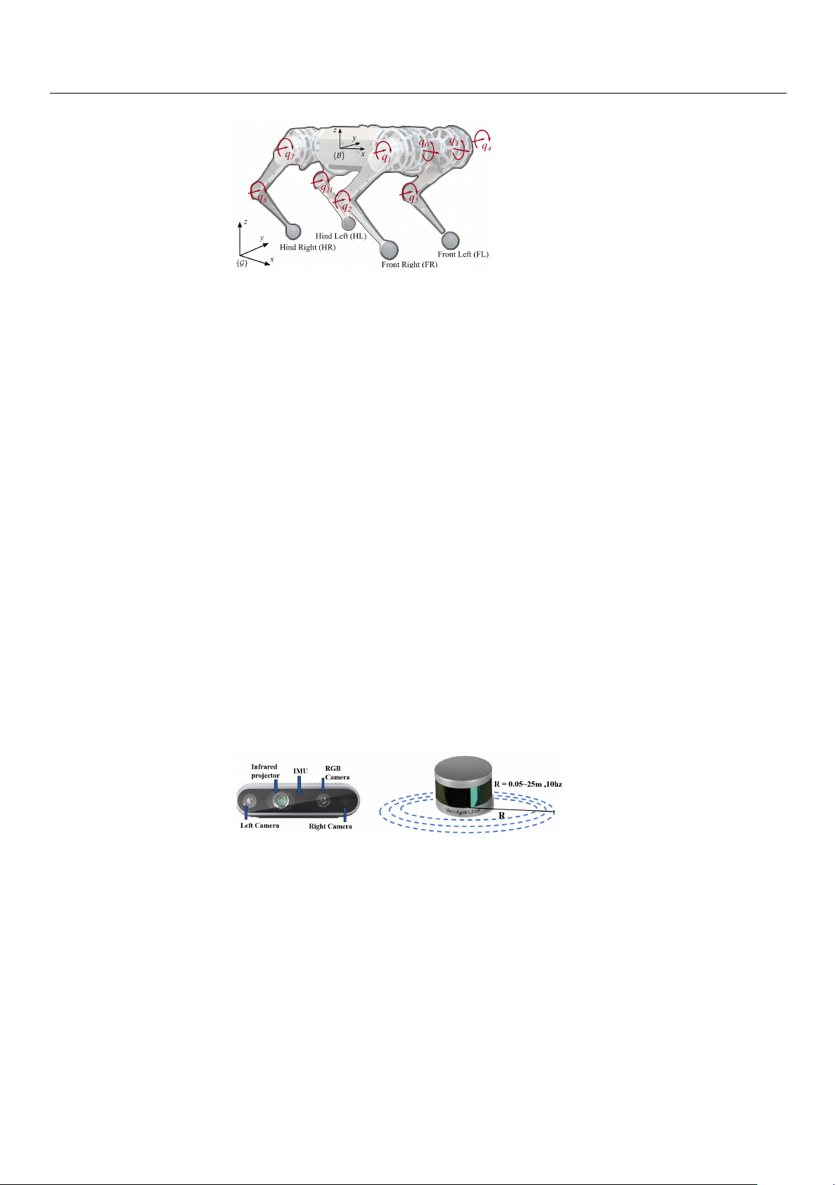
4.1. Sensory Information Acquisition
In this module, sensory data are primarily acquired using the Intel RealSense D435i
depth camera, which is integrated with a six-DOF IMU. The combination of depth sensing
and pose estimation provides the robot with high-density point cloud data.
The D435i captures depth information using infrared and RGB cameras. By projecting
structured light and using triangulation, the system generates a 3D point cloud, where each
point is represented by p = (x, y, z). Meanwhile, the integrated IMU provides six-DoF data:
linear acceleration in three axes and angular velocity. The robot’s orientation is estimated
using quaternions q = (qx, qy, qz, qw), while the IMU’s accelerometers and gyroscopes
measure the robot’s linear and angular motion.
For comparison purposes, Figure 7 shows a velodyne LiDAR sensor, which is also
incorporated into the experiments. The LiDAR is configured as a 360-degree scanning 2D
sensor, with a scanning frequency of 10 Hz and a measurement range from 0.05 m to 25 m.
Although the LiDAR-generated point cloud is sparser than that of the D435i, it performs
well in detecting distant obstacles [40].
Figure 7. Intel D435i and velodyne LIDAR. 4.2. Grid Map Construction
After obtaining the point cloud data and pose information from the camera, the next
step involves constructing a real-time updated grid map. This section explains the 3D-3D
pose estimation process and the grid map generation method, which forms the foundation
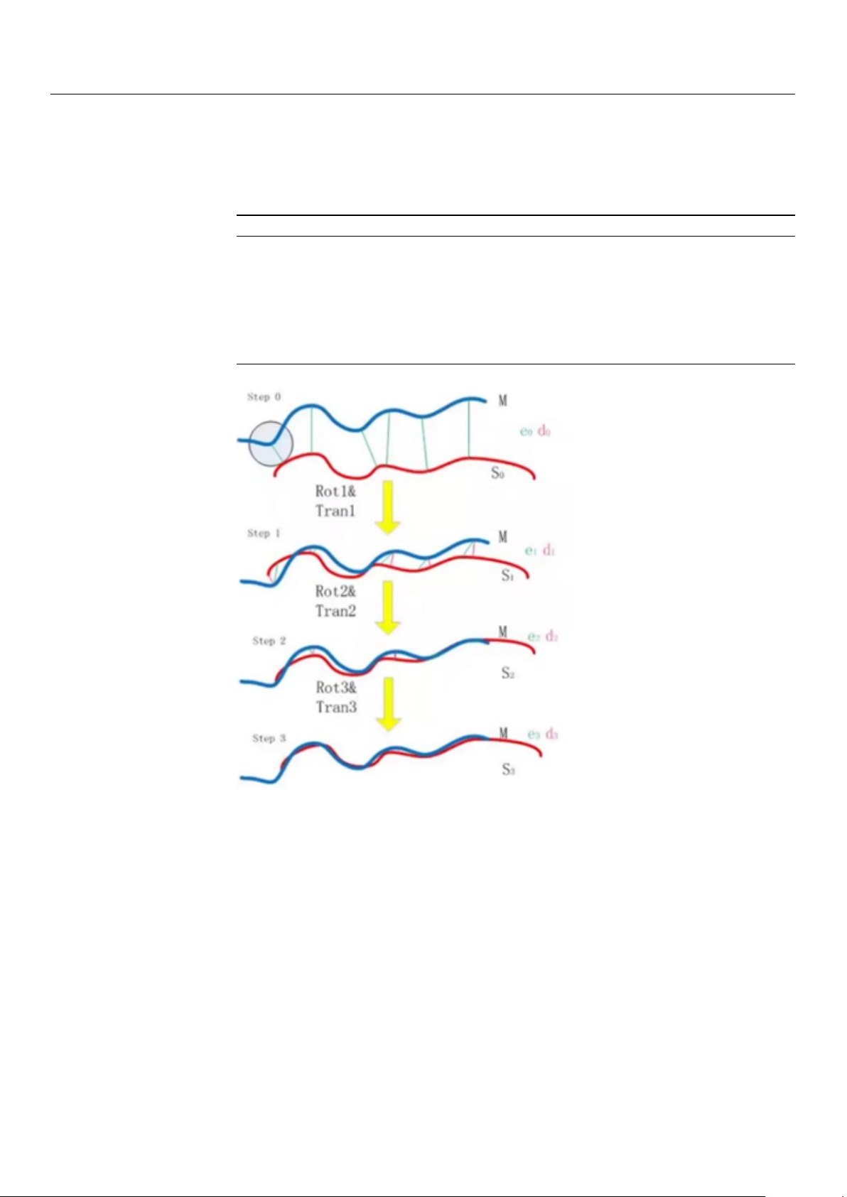
for robot navigation and mapping. The 3D-3D Pose Estimation
The Iterative Closest Point (ICP) algorithm is employed to match the point clouds be-
tween different frames. This algorithm iteratively refines the alignment of two point clouds
by minimizing the distance between corresponding points. The ICP process begins with
an initial guess of the rotation (R) and translation (T), as demonstrated in the pseudocode
shown in Algorithm 1 and the corresponding diagram in Figure 8. In each iteration, a point Sensors 2024, 24, 7306 13 of 32
from the first point cloud is matched with the nearest point in the second point cloud, and
the transformation is updated based on these correspondences. The iteration continues
until the error converges to a minimal value or the maximum number of iterations is
reached, resulting in an aligned point cloud.
Algorithm 1 ICP Processing Flow
1: Initialize: Initial Guess for Rotation R and Translation T
2: while error not converged or max iterations not reached do
3: For each point p1 in PointCloud1, find the nearest point p2 in PointCloud2
4: Compute the difference between corresponding points
5: Update rotation R and translation T based on the computed differences 6: end While
7: Output the final aligned PointCloud Figure 8. ICP diagram.
During data association, the nearest neighbor search is typically used to find the
corresponding points between two point clouds. This approach calculates the Euclidean
distance for each point, which has a computational complexity of O(N). However, when
the same dataset is queried repeatedly, the Kd-tree data structure can be employed to
optimize the search, reducing the complexity to O(log N). This optimization reduces the
computational load, making the process more efficient for large datasets.
4.3. Grid Map Construction and Inflation Handling
Before constructing the grid map, point cloud data are captured using a depth camera,
and the map is stored in an OccupancyMap format, where each cell is marked as either free
(0) or occupied (1). To simplify computations, it is assumed that the map is static and that
each cell is independent. While this method places significant memory pressure on the
processor and cannot store continuous obstacle information efficiently, it remains effective
for planar obstacle detection in ground-based robot experiments. Sensors 2024, 24, 7306 14 of 32
After generating the grid map, local inflation is applied to ensure safe obstacle avoid-
ance. We modify the parameter ‘obstaclein f lation = 0.5’, and the map inflates around
obstacles, ensuring that the robot maintains a safe distance during path planning. Figure 9
shows the initial grid map, and Figure 9 shows the map after inflation. The inflation
algorithm focuses on the robot’s forward field of view, which is approximately 60 degrees,
optimizing processing by ignoring unnecessary regions. After inflation, the perception
module ensures a sufficient safety margin to avoid collisions during navigation.
Figure 9. Comparison of before and after modifying the perception region.
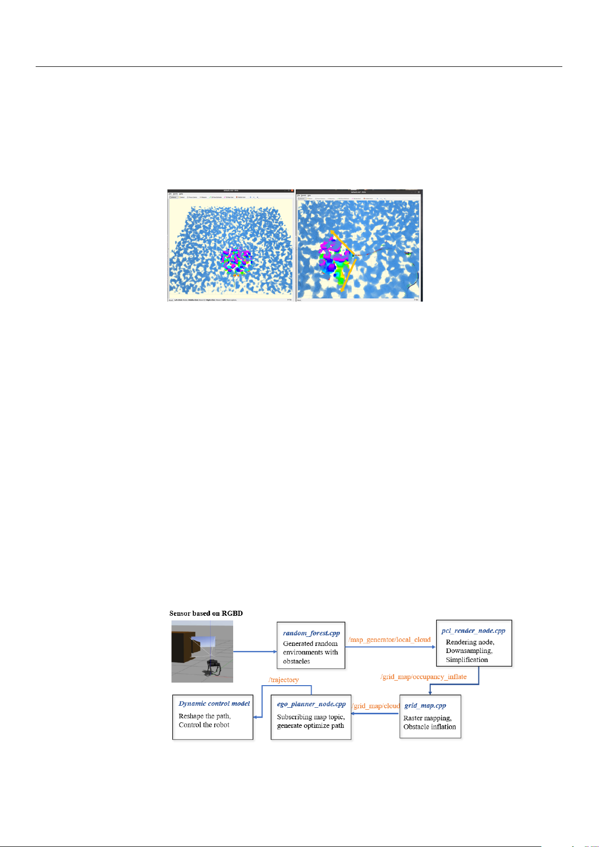
4.4. Sensory Information Communication in ROS
During the grid map generation process, techniques such as point cloud preprocessing
and overlap detection were utilized to manage the high-density data generated by the depth
camera. These point cloud data, significantly more complex than the LiDAR data, required
downsampling to alleviate system processing pressures. The unordered multidimensional
array format of the point cloud posed computational challenges during map rendering.
To improve efficiency, a KD-tree was used to associate the data, simplifying the
subsequent processing steps. The primary implementation of this process is handled by the
pcl_cloud_render.cpp file, which processes raw point cloud data from the grid map. PCL
(Point Cloud Library) rendering applies downsampling and density reduction, ensuring
that the processed point cloud data conform to the required format for robot perception.
We use a KD tree to build the data structure, facilitating fast nearest neighbor searches.
And the PCL was used for downsampling and density reduction, ensuring that the pro-
cessed point cloud data conform to the required format for the perception system.
After preprocessing, the filtered point cloud is returned to the grid map for further in-
flation. The inflated map is then published to the ROS topic grid_map/occupancy_inflate,
allowing the quadruped robot’s 2D EGO-Planner to use the map for trajectory planning.
As shown in Figure 10, the system subscribes to relevant topics, processes sensory data,
and performs obstacle inflation. The expanded grid map, along with the original PCL data,
is broadcast in PCL format. With the completion of the grid map generation and obstacle
inflation processes, the system is now fully prepared for trajectory search and execution.
Figure 10. Point cloud processing flowchart. Sensors 2024, 24, 7306 15 of 32 4.5. EGO-Planner
In this section, we provide a detailed overview of the complete trajectory generation
process. We incorporate modifications to the 2D EGO-Planner to meet the robot’s requirements
for planar motion. The overall planning framework employs a multi-layered path planning
approach, which includes both global path planning and local trajectory optimization. Trajectory Generation Process
In the global path planning phase, the system employs a dynamic A* algorithm to
generate an initial global path. This algorithm operates on a grid map to produce a rough
path from the start point to the target destination. Although this path does not fully account
for the robot’s dynamic constraints, it effectively avoids the static obstacles present in the
initial grid map, thus providing directional guidance for subsequent local optimization.
The resulting discrete path points serve as the initial input for the EGO-Planner, which will
perform further local refinements.
In the local path planning phase, the EGO-Planner refines the initial path using real-
time environmental data and the trajectory provided by the A* algorithm [41]. The primary
function of the EGO-Planner is to generate a B-spline curve that smooths and optimizes the
path while ensuring collision avoidance [42]. When a control point detects a collision with
an obstacle, the system employs gradient descent to move the point away from the obstacle.
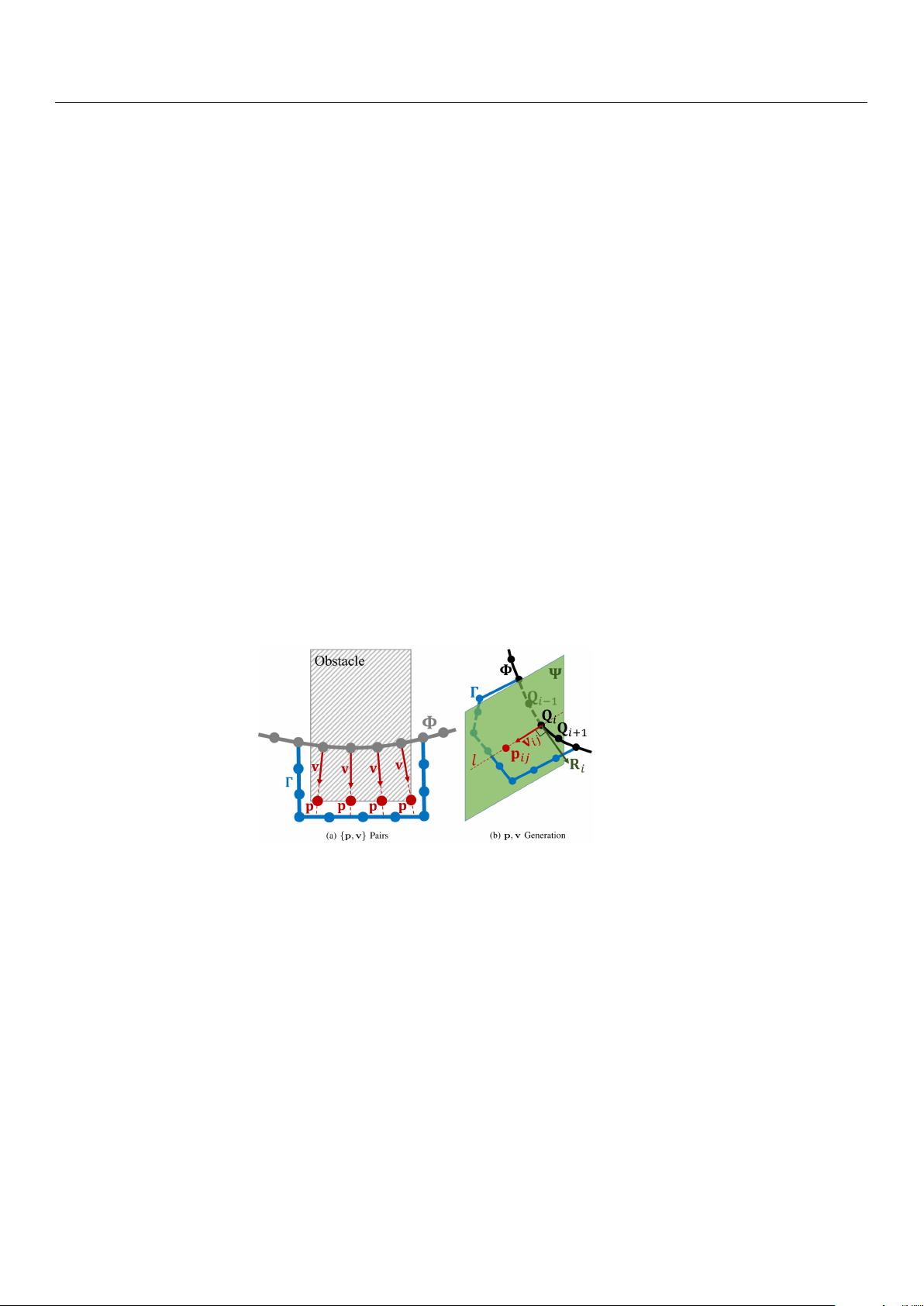
Specifically, as illustrated in Figure 11a, for each collision point, an anchor point
pij is generated on the obstacle surface. The system then calculates a repulsive vector
vij that directs the control point away from the obstacle, pushing it to a safer location:
vij = f (pij, Qi), where pij is the anchor point on the obstacle surface, and Qi is the collision-
detected control point. This dynamic update of the {p, v} pairs allows the trajectory to be
iteratively adjusted, forming a collision-free path.
Figure 11. {p, v} generation: (a) the creation of {p, v} pairs for collision points; (b) the process of
generating anchor points and repulsive vectors for dynamic obstacle avoidance [41].
Figure 11b further illustrates the process of generating anchor points pij and repulsive
vectors vij in a 3D space. The control point Qi is first identified as a collision point. In
a 3D space, the anchor point pij is positioned on the surface of the obstacle, close to the
projection of the control point Qi along the path Γ. The system then calculates the repulsive
vector vij from the control point to the anchor point, thereby modifying the position of Qi
to ensure that it moves away from the obstacle.
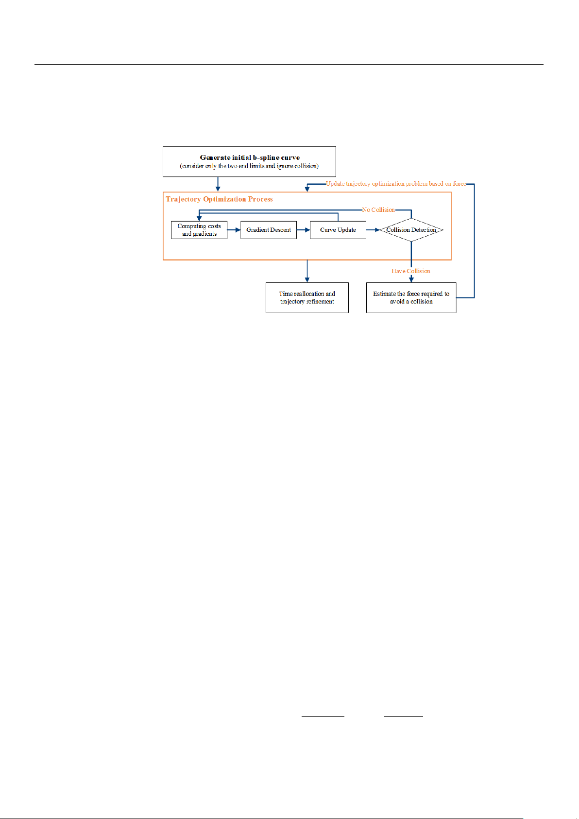
To handle complex terrains and dynamic obstacles, the EGO-Planner continuously
updates the trajectory’s control points based on real-time sensory input. As shown in
Figure 12, this adjustment process is not a one-time event but involves multiple iterations
based on continuous feedback from the environment. During each iteration, the system
performs collision detection, cost computation, and curve updates until the path satisfies
the collision avoidance requirements.
To meet both spatial and dynamic requirements, the EGO-Planner incorporates a
time reallocation mechanism. As shown in Figure 12, this mechanism optimizes the time
intervals ∆t between control points {Q1, Q2, . . . , QN } based on the computed derivatives c Sensors 2024, 24, 7306 16 of 32 ... (velocity ˙ Q(t), acceleration ¨
Q(t), and jerk Q(t)) at each time step. By adjusting these inter-
vals, the trajectory maintains smoothness while adhering to dynamic feasibility constraints.
The control points’ velocities ˙
Qi correspond to each time interval ∆ti, ensuring that changes
in speed, acceleration, and jerk are within the system’s limits.
Figure 12. Overall framework of 2D EGO-Planner.
Once the control points have been adjusted to avoid obstacles, the system proceeds to
merge these points with the unaffected segments of the original path. This merging process
takes advantage of the convex hull property of B-splines to ensure a smooth transition
between the modified and original segments.
In the EGO-Planner, the trajectory is modeled using uniform B-spline curves ϕ. These
curves are defined by the order pb, the control points {Q1, Q2, . . . , QN }, and a knot vector c {t 3
1, t2, . . . , tM}, where Qi ∈ R , tm ∈ R, and M = Nc + pb. Each node of the B-spline
curve has an equal time interval, ∆t = tm+1 − tm. The convex hull property of B-spline
curves allows for a smooth merging of the modified and original path segments during trajectory optimization.
The dynamic properties of the trajectory, including velocity ˙p and acceleration ¨p, are
derived directly from the control points of the B-spline curve. To ensure that the trajectory
satisfies dynamic constraints, the EGO-Planner uses a time reallocation mechanism, adjust-
ing the time intervals ∆t between the control points to regulate velocity ˙p, acceleration ¨p,
and jerk, maintaining smoothness and dynamic feasibility.
4.6. Improvements in EGO-Planner The 2D EGO-Planner
In practice, the A* algorithm is confined to searching within a 2D plane, simplifying
the path generation process. However, the obstacle detection module operates with a 3D
grid map, which accurately represents the surrounding environment. The workflow of
the 2D EGO-Planner begins by initializing control points Q = {Q1, Q2, . . . , Qn} in a 2D
space to form the initial path. While the planner generates the path in 2D, the obstacle
detection module continuously updates the 3D grid map using real-time sensor data to
identify obstacle segments S. Algorithm 2 shows that, for each detected obstacle segment,
the system computes repulsive forces, generating anchor points pij and repulsive vectors
vij. These forces are then used to optimize the B-spline curve in the 2D plane. In this
2D context, the system evaluates dynamic constraints by computing the first and second
derivatives of the B-spline control points: Q V V i+1 − Qi i+1 − Vi i = ∆ , A . (17) t i = ∆t Sensors 2024, 24, 7306 17 of 32
The optimization process iteratively adjusts both the control points and the time intervals
∆t to ensure compliance with velocity and acceleration constraints.
Algorithm 2 2D-EGO-Planner for Ground Robots
1: Initialize: Q (Control Points in 2D), Env (Environment), goal
2: while not reached goal do 3:
S ← Detect Obstacle Segments in 2D 4:
for all segments in S do 5:
p, v ← Find Repulsive Force (S) 6:
Update Control Points: Q ← Optimize B-spline trajectory in 2D 7: end for 8:
if Trajectory violates dynamic constraints then 9:
Adjust Time Allocation and Refine Trajectory 10: end if 11: Move to next waypoint 12: end while
During each iteration, a feedback loop continuously evaluates the trajectory for viola-
tions of dynamic constraints. The control points are refined to ensure dynamic feasibility,
while the time intervals are reallocated when necessary, maintaining an optimized path
until the target point is reached. 5. Results 5.1. Robot Assembly
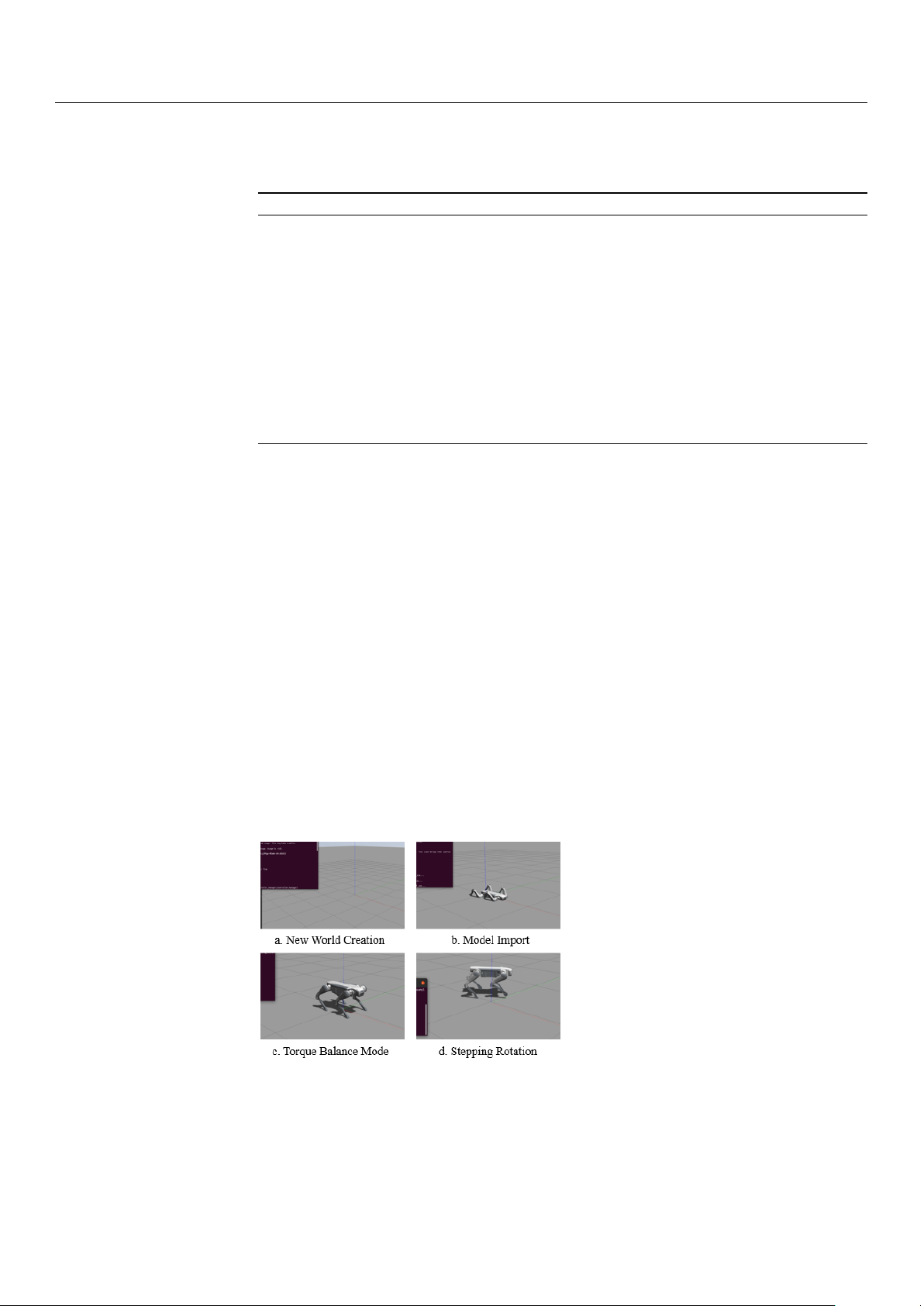
After the establishment of the ROS node communication system, we can build the robot
dog model while completing some simple movement practices. The robot initialization
process is shown in detail in Figure 13. Firstly, the world model is launched to create
a Gazebo simulation environment; then, we input the robot model into the simulation.
Afterwards, the torque balance command is given by a keyboard, and the commands are
transmitted to the actuator via the serial communication protocol. The actuator adjusts the
joint torque according to the received commands to ensure that the robot dog can remain
stable on different surfaces. Lastly, the trot command is given by a keyboard command.
At this time, the robot dog will follow the speed given in the command velocity topic to
control the CoM to reach the target position and orientation. During operation, by reading
the information on the terminal, it can be seen that the robot dog’s delay is less than 25 ms.
Figure 13. Robot initialization and control process in Gazebo simulation: (a) Gazebo environment
creation, (b) robot model import, (c) torque balance mode activation, and (d) robot stepping and rotation in simulation. 5.2. Robot Control
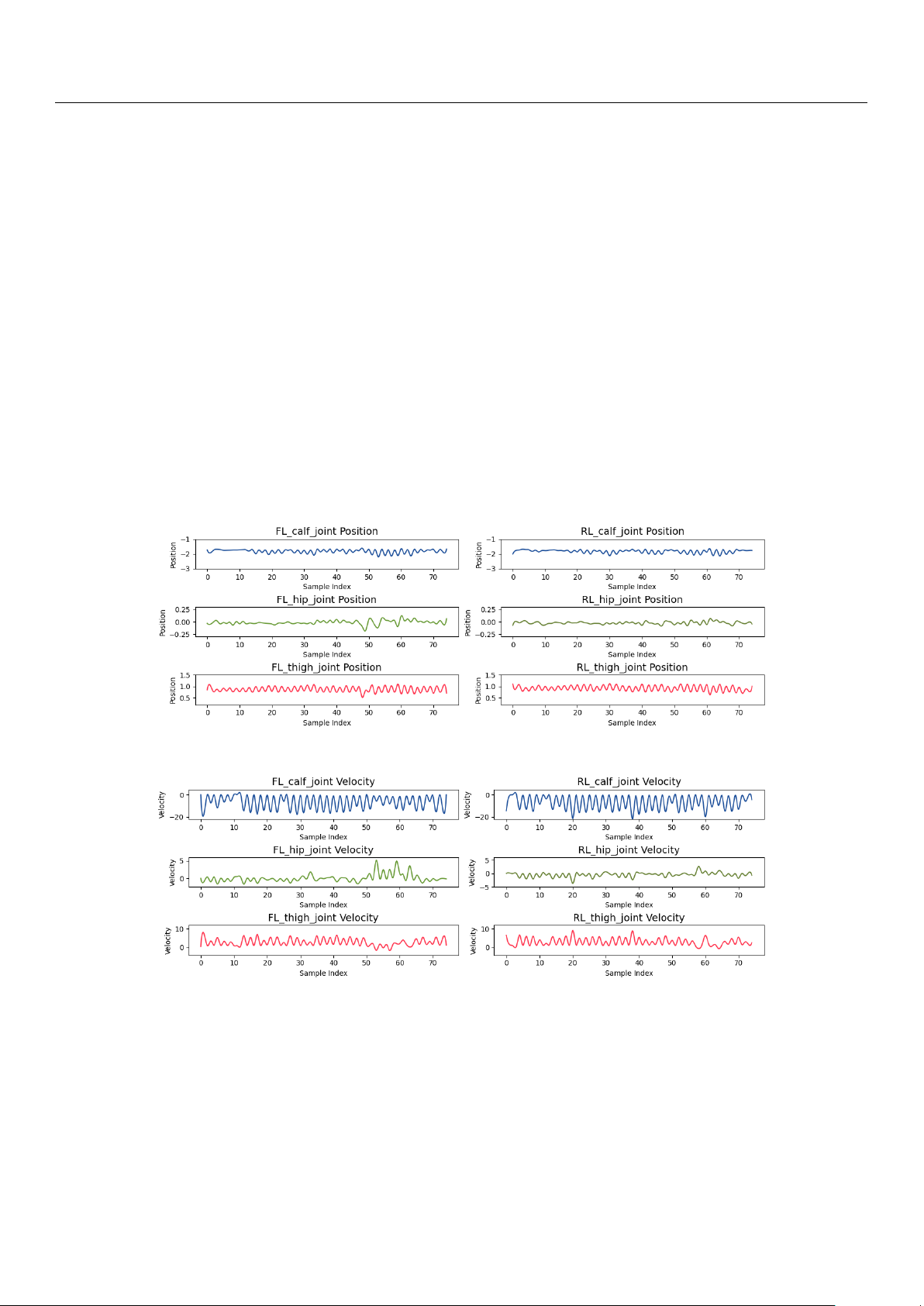
The experiment in this section analyzes the motion control of the quadruped robot’s
front-left (FL) and rear-left (RL) leg joints, focusing on the distribution of the CoM trajectory. Sensors 2024, 24, 7306 18 of 32
The joint positions, as shown in Figure 14, exhibit periodic oscillations, demonstrating
the regularity of leg movements during the gait cycle. For example, the FL_thigh_joint
oscillates between 0.5 and 1.5 radians, while the FL_calf_joint shows a larger range from
−2.5 to −1.0 radians, indicating more significant motion during transitions. This periodic
behavior is similarly observed in other joints, clearly reflecting the different stages of the gait cycle.
The following figures present data from an experiment in which the quadruped robot
autonomously navigated a simple environment, successfully avoiding static obstacles.
During this experiment, the robot performed a basic turning maneuver while maintaining
stability and control, as reflected in the joint positions, velocities, and torques.
Figure 14 shows that the joint positions of the front-left (FL) and rear-left (RL) legs
exhibit periodic oscillations, typical of a gait cycle. For example, the FL_thigh_joint oscil-
lates between 0.5 and 1.5 radians, while the FL_calf_joint shows a larger range from −2.5 to
−1.0 radians, indicating more significant motion during stance and swing transitions. This
behavior is consistent across other joints, reflecting the different phases of the gait cycle.
Joint angular velocities, while still periodic, exhibit smaller fluctuations (Figure 15).
The RL_calf_joint oscillates between −20 and 0 rad/s, peaking during leg lifting and
lowering, indicating intensive movement. The FL_thigh_joint, however, remains more
stable, oscillating between 0 and 10 rad/s, reflecting its role in providing steady support.
Figure 14. Joint rotational angles of FL and RL legs.
Figure 15. Joint angular velocities of FL and RL legs.
Torque, as shown in Figure 16, provides further insight into external loads during
motion. The FL_calf_joint experiences torque variations from −25 to 20 Nm, reflecting the
load changes during leg lifting and weight bearing. In contrast, the RL_hip_joint shows
relatively smaller torque variations, maintaining stability throughout the gait.
These results indicate that the robot’s motion control system efficiently allocates the
CoM trajectory to the joints, allowing for stable and controlled gait execution across various phases of the cycle. Sensors 2024, 24, 7306 19 of 32
Figure 16. Torque applied to FL and RL joints during the gait cycle.
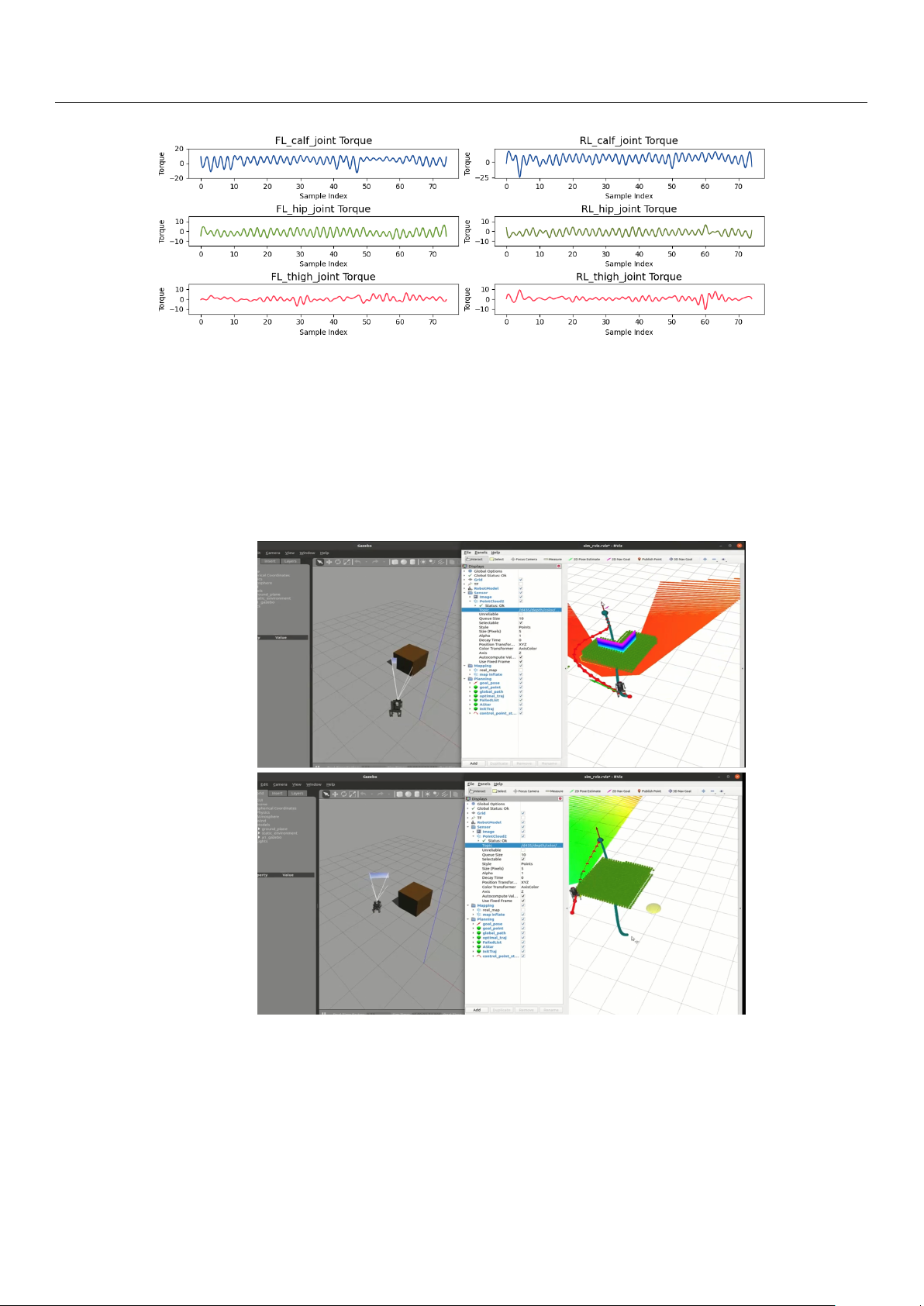
5.3. RGB-D-Based Autonomous Navigation in Static Environment
This section introduces the RGB-D-based autonomous navigation. Figures 17 and 18
illustrate the initial path planning and dynamic replanning process when encountering
simple obstacles. In the initial state, the path planner generates a baseline trajectory without
considering collisions. As the robot moves along this trajectory and detects obstacles, the
state machine transitions from the EXEC_TRAJ state to the REPLAN_TRAJ state, prompting
the planner to update the CoM trajectory to ensure obstacle avoidance.
Figure 17. The robot navigating in a simple environment using a camera. Sensors 2024, 24, 7306 20 of 32
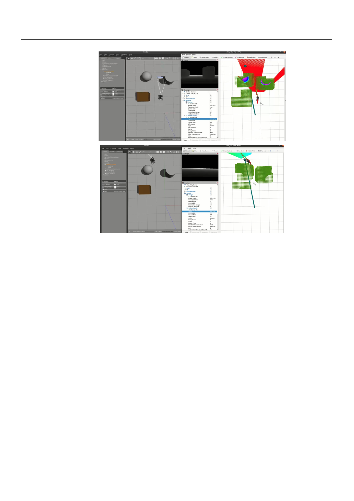
Figure 18. The robot navigating in a complex environment using a camera.
Based on the preliminary D* path, the 2D EGO-Planner computes a safe trajectory
around the detected obstacles. Figure 17 shows the robot’s progress through the environ-
ment, successfully navigating towards the target position while avoiding obstacles. As
shown in Figure 18, the Gazebo interface shows how the D435i camera mounted on the
robot detects the obstacles in real time. The system performs real-time replanning when
necessary, with an average of 35 iterations per robo_plan, typically completing the entire
navigation process, including 200 iterations of robo_plan, within 15 s. Due to the limita-
tions of the experimental platform, prolonged operation may lead to system instability.
Therefore, we constrained the robot’s movement to a small but characteristic environment
with distinct obstacles to evaluate its performance. Despite the limited time frame, the
experiment demonstrates a complete autonomous navigation process, showcasing the
robot’s ability to efficiently avoid obstacles and adjust its trajectory in real time.
Additionally, we optimized the robot’s velocity limits to ensure stability during ex-
ecution. The velocity thresholds were set at vx, vy = 0.5 m/s, as higher thresholds led to
instability. This configuration provided an optimal balance between speed and naviga- tion safety.
Figure 19 illustrates the complete trajectory in a 2D plane. Initially, a rough path (black
line) is generated based on the start and goal positions. The green shaded rectangle indicates
an artificially set obstacle and its inflated boundary, which aligns with the obstacles in the
Gazebo simulation. The red points represent predefined target points, while the blue points
denote the planner’s output path.
The robot dynamically adjusts its path to avoid collisions, maintaining the replanning
time for each iteration within 10 milliseconds to ensure real-time performance. Each
iteration represents the time it takes for the robot, in the robo_plan state, to compute the
trajectory points for the next time step. Given that a typical experiment involves multiple
instances of this replanning process, this demonstrates the system’s ability to consistently
perform real-time trajectory adjustments. The red points represent predefined target points,
while the blue points denote the planner’s output path.