International Monetary Arrangements - Key Concepts and History | Tài chính quốc tế | Trường Học Viện nông nghiệp Việt Nam
Like most areas of public policy, international monetary relations are subject to frequent proposals for change. Fixed exchange rates, floating exchange rates, and commodity-backed currency all have their advocates. Before considering the merits of alternative international monetary systems, we should understand the background of the international monetary system. Tài liệu được sưu tầm và soạn thảo dưới dạng file PDF để gửi tới các bạn cùng tham khảo, ôn tập đầy đủ kiến thức, chuẩn bị cho các buổi học thật tốt. Mời bạn đọc đón xem!
Môn: Tài chính quốc tế (hvnn) 130 tài liệu
Trường: Học viện Nông nghiệp Việt Nam 2.4 K tài liệu
Tác giả:
Preview text:
CHAPTER 2 International Monetary Arrangements Contents
The Gold Standard: 1880–1914 25
The Interwar Period: 1918–1939 28
The Bretton Woods Agreement: 1944–1973 29
Central Bank Intervention During Bretton Woods 30
The Breakdown of the Bretton Woods System 33
The Transition Years: 1971–1973 33
International Reserve Currencies 34
Post Bretton Woods: 1973 to the Present 39
The Choice of an Exchange Rate System 41
Currency Boards and “Dollarization” 45 Optimum Currency Areas 48
The European Monetary System and the Euro 49 Summary 51 Exercises 52 Further Reading 53
Appendix A Current Exchange Rate Arrangements 53
Like most areas of public policy, international monetary relations are
subject to frequent proposals for change. Fixed exchange rates, floating
exchange rates, and commodity-backed currency all have their advocates.
Before considering the merits of alternative international monetary sys-
tems, we should understand the background of the international monetary
system. Although an international monetary system has existed since mon-
ies have been traded, it is common for most modern discussions of inter-
national monetary history to start in the late 19th century. It was during
this period that the gold standard began.
THE GOLD STANDARD: 1880–1914
Although an exact date for the beginning of the gold standard cannot be
pinpointed, we know that it started during the period from 1880 to 1890. © 201 7 Elsevier Inc.
International Money and Finance. All rights reserved. 25 26
International Money and Finance
Under a gold standard, currencies are valued in terms of their gold equiva-
lent (an ounce of gold was worth $20.67 in terms of the US dollar over
the gold standard period). The gold standard is an important beginning for
a discussion of international monetary systems because when each cur-
rency is defined in terms of its gold value, all currencies are linked in a
system of fixed exchange rates. For instance, if currency A is worth 0.10
ounce of gold, whereas currency B is worth 0.20 ounce of gold, then
1 unit of currency B is worth twice as much as 1 unit of A, and thus the
exchange rate of 1 currency B = 2 currency A is established.
Maintaining a gold standard requires a commitment from participating
countries to be willing to buy and sell gold to anyone at the fixed price.
To maintain a price of $20.67 per ounce, the United States had to buy
and sell gold at that price. Gold was used as the monetary standard because
it is a homogeneous commodity (could you have a fish standard?) world-
wide that is easily storable, portable, and divisible into standardized units
like ounces. Since gold is costly to produce, it possesses another important
attribute—governments cannot easily increase its supply. A gold standard is
a commodity money standard. Money has a value that is fixed in terms of the commodity gold.
One aspect of a money standard that is based on a commodity with
relatively fixed supply is long-run price stability. Since governments must
maintain a fixed value of their money relative to gold, the supply of
money is restricted by the supply of gold. Prices may still rise and fall with
swings in gold output and economic growth, but the tendency is to return
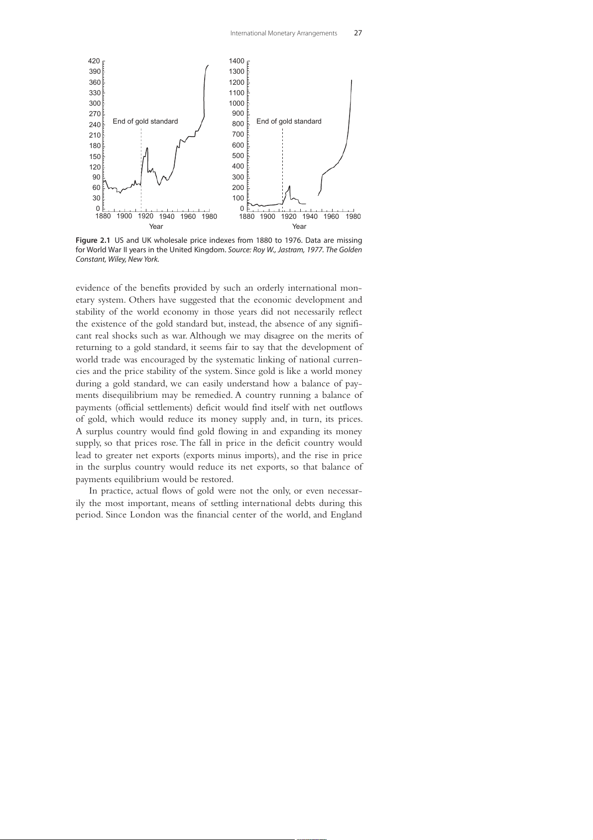
to a long-run stable level. Fig. 2.1 illustrates graphically the relative stabil-
ity of US and UK prices over the gold standard period as compared to
later years. However, note also that prices fluctuated up and down in the
short run during the gold standard. Thus, frequent small bursts of inflation
and deflation occurred in the short run, but in the long run the price level
remained unaffected. Since currencies were convertible into gold, national
money supplies were constrained by the growth of the stock of gold. As
long as the gold stock grew at a steady rate, prices would also follow a
steady path. New discoveries of gold would generate discontinuous jumps
in the price level, but the period of the gold standard was marked by a fairly stable stock of gold.
People today often look back on the gold standard as a “golden era” of
economic progress. It is common to hear arguments supporting a return
to the gold standard. Such arguments usually cite the stable prices, eco-
nomic growth, and development of world trade during this period as
International Monetary Arrangements 27 420 1400 390 1300 360 1200 330 1100 300 1000 x 270 x 900 e e d End of gold standard End of gold standard 240 d 800 in in 210 700 rice rice p 180 p 600 S K U 150 U 500 120 400 90 300 60 200 30 100 0 0 1880 1900 1920 1940 1960 1980 1880 1900 1920 1940 1960 1980 Year Year
Figure 2.1 US and UK wholesale price indexes from 1880 to 1976. Data are missing
for World War II years in the United Kingdom. Source: Roy W., Jastram, 1977. The Golden Constant, Wiley, New York.
evidence of the benefits provided by such an orderly international mon-
etary system. Others have suggested that the economic development and
stability of the world economy in those years did not necessarily reflect
the existence of the gold standard but, instead, the absence of any signifi-
cant real shocks such as war. Although we may disagree on the merits of
returning to a gold standard, it seems fair to say that the development of
world trade was encouraged by the systematic linking of national curren-
cies and the price stability of the system. Since gold is like a world money
during a gold standard, we can easily understand how a balance of pay-
ments disequilibrium may be remedied. A country running a balance of
payments (official settlements) deficit would find itself with net outflows
of gold, which would reduce its money supply and, in turn, its prices.
A surplus country would find gold flowing in and expanding its money
supply, so that prices rose. The fall in price in the deficit country would
lead to greater net exports (exports minus imports), and the rise in price
in the surplus country would reduce its net exports, so that balance of
payments equilibrium would be restored.
In practice, actual flows of gold were not the only, or even necessar-
ily the most important, means of settling international debts during this
period. Since London was the financial center of the world, and England 28
International Money and Finance
the world’s leading trader and source of financial capital, the pound also
served as a world money. International trade was commonly priced in
pounds, and trade that never passed through England was often paid for with pounds.
THE INTERWAR PERIOD: 1918–1939
World War I ended the gold standard. International financial relations are
greatly strained by war, because merchants and bankers must be concerned
about the probability of countries suspending international capital flows.
At the beginning of the war both the patriotic response of each nation’s
citizens and legal restrictions stopped private gold flows. Since wartime
financing required the hostile nations to manage international reserves
very carefully, private gold exports were considered unpatriotic. Central
governments encouraged (and sometimes mandated) that private holders
of gold and foreign exchange sell these holdings to the government.
Because much of Europe experienced rapid inflation during the war
and in the period immediately following it, it was not possible to restore
the gold standard at the old exchange values. However, the United
States had experienced little inflation and thus returned to a gold stan-
dard by June 1919. The war ended Britain’s financial preeminence, since
the United States had risen to the status of the world’s dominant banker
country. In the immediate postwar years the pound fluctuated freely
against the dollar in line with changes in the price level of each country.
In 1925, England returned to a gold standard at the old prewar pound
per gold exchange rate, even though prices had risen since the pre-
war period. As John Maynard Keynes had correctly warned, the overval-
ued pound hurt UK exports and led to a deflation of British wages and
prices. By 1931, the pound was declared inconvertible because of a run
on British gold reserves (a large demand to convert pounds into gold), and
so ended the brief UK return to a gold standard. Once the pound was no
longer convertible into gold, attention centered on the US dollar. A run
on US gold at the end of 1931 led to a 15% drop in US gold holdings.
Although this did not lead to an immediate change in US policy, by 1933
the United States abandoned the gold standard.
The depression years were characterized by international monetary
warfare. In trying to stimulate domestic economies by increasing exports,
country after country devalued, so that the early to mid-1930s may be
International Monetary Arrangements 29
characterized as a period of competitive devaluations. Governments also
resorted to foreign exchange controls in an attempt to manipulate net
exports in a manner that would increase gross domestic product (GDP).
Of course, with the onslaught of World War II, the hostile countries
utilized foreign exchange controls to aid the war-financing effort.
THE BRETTON WOODS AGREEMENT: 1944–1973
Memories of the economic warfare of the interwar years led to an inter-
national conference at Bretton Woods, New Hampshire, in 1944. At the
close of World War II there was a desire to reform the international mon-
etary system to one based on mutual cooperation and freely convertible currencies.
There was a need for a system that fixed currencies relative to each
other, but did not fix each currency in terms of gold. The Bretton Woods
agreement solved this problem by requiring that each country fix the
value of its currency in terms of an anchor currency, namely the dollar
(this established the “par” value of each currency and was to ensure parity
across currencies). The US dollar was the key currency in the system, and
$1 was defined as being equal in value to 1/35 ounce of gold. Since every cur-
rency had an implicitly defined gold value, through the link to the dollar,
all currencies were linked in a system of fixed exchange rates.
Nations were committed to maintaining the parity value of their
currencies within 1% of parity. The various central banks were to
achieve this goal by buying and selling their currencies (usually against
the dollar) on the foreign exchange market. When a country was experi-
encing difficulty maintaining its parity value because of balance of pay-
ments disequilibrium, it could turn to a new institution created at the
Bretton Woods Conference: the International Monetary Fund (IMF). The
IMF was created to monitor the operation of the system and provide
short-term loans to countries experiencing temporary balance of pay-
ments difficulties. Such loans are subject to IMF conditions regarding
changes in domestic economic policy aimed at restoring balance of pay- ments equilibrium.
In the case of a fundamental disequilibrium, when the balance of pay-
ments problems are not of a temporary nature, a country could apply
for permission from the IMF to devalue or revalue its currency. Such a
permanent change in the parity rate of exchange was rare. Table 2.1 30
International Money and Finance
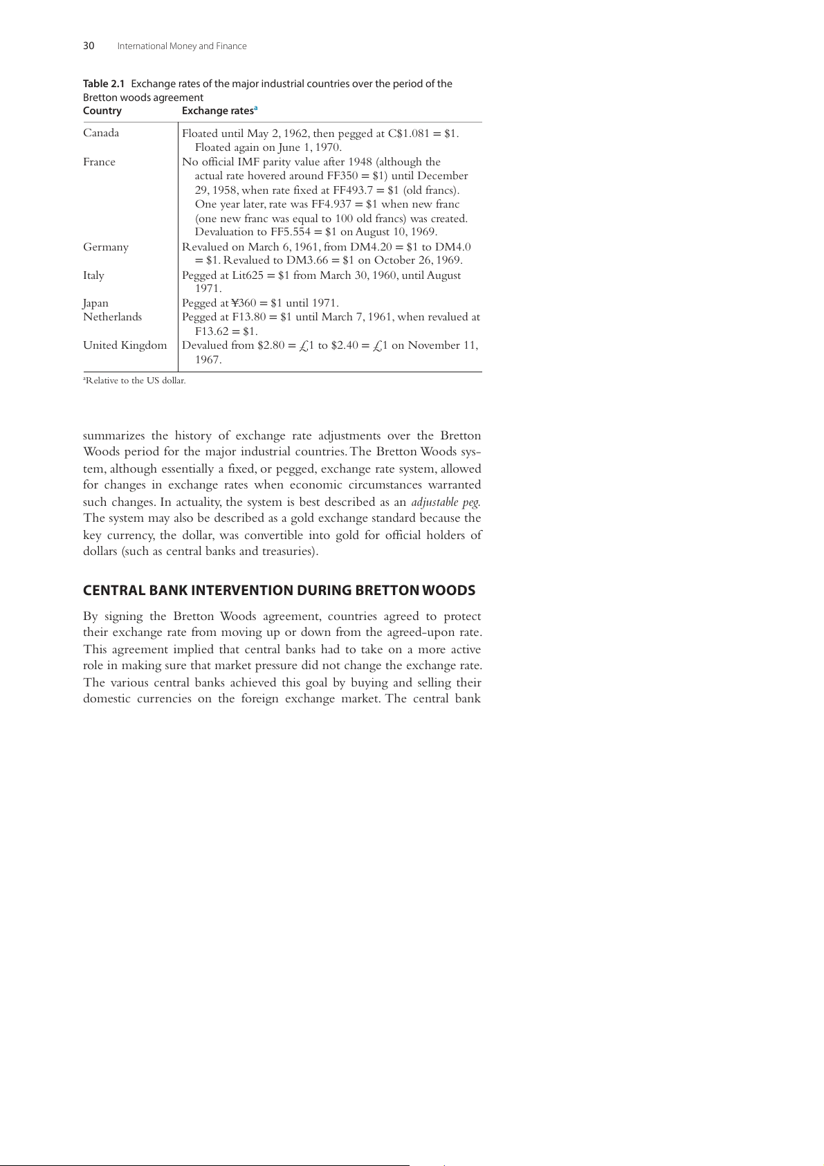
Table 2.1 Exchange rates of the major industrial countries over the period of the Bretton woods agreement Country Exchange ratesa Canada
Floated until May 2, 1962, then pegged at C$1.081 = $1. Floated again on June 1, 1970. France
No official IMF parity value after 1948 (although the
actual rate hovered around FF350 = $1) until December
29, 1958, when rate fixed at FF493.7 = $1 (old francs).
One year later, rate was FF4.937 = $1 when new franc
(one new franc was equal to 100 old francs) was created.
Devaluation to FF5.554 = $1 on August 10, 1969. Germany
Revalued on March 6, 1961, from DM4.20 = $1 to DM4.0
= $1. Revalued to DM3.66 = $1 on October 26, 1969. Italy
Pegged at Lit625 = $1 from March 30, 1960, until August 1971. Japan
Pegged at ¥360 = $1 until 1971. Netherlands
Pegged at F13.80 = $1 until March 7, 1961, when revalued at F13.62 = $1. United Kingdom
Devalued from $2.80 = £1 to $2.40 = £1 on November 11, 1967. aRelative to the US dollar.
summarizes the history of exchange rate adjustments over the Bretton
Woods period for the major industrial countries. The Bretton Woods sys-
tem, although essentially a fixed, or pegged, exchange rate system, allowed
for changes in exchange rates when economic circumstances warranted
such changes. In actuality, the system is best described as an adjustable peg.
The system may also be described as a gold exchange standard because the
key currency, the dollar, was convertible into gold for official holders of
dollars (such as central banks and treasuries).
CENTRAL BANK INTERVENTION DURING BRETTON WOODS
By signing the Bretton Woods agreement, countries agreed to protect
their exchange rate from moving up or down from the agreed-upon rate.
This agreement implied that central banks had to take on a more active
role in making sure that market pressure did not change the exchange rate.
The various central banks achieved this goal by buying and selling their
domestic currencies on the foreign exchange market. The central bank
International Monetary Arrangements 31 The Market for British Pounds S$/£ S1(£) S2(£) Intervention A C 2.00 1.80 B D (£) 1 Q1 Q2 Q3 Quantities of pound
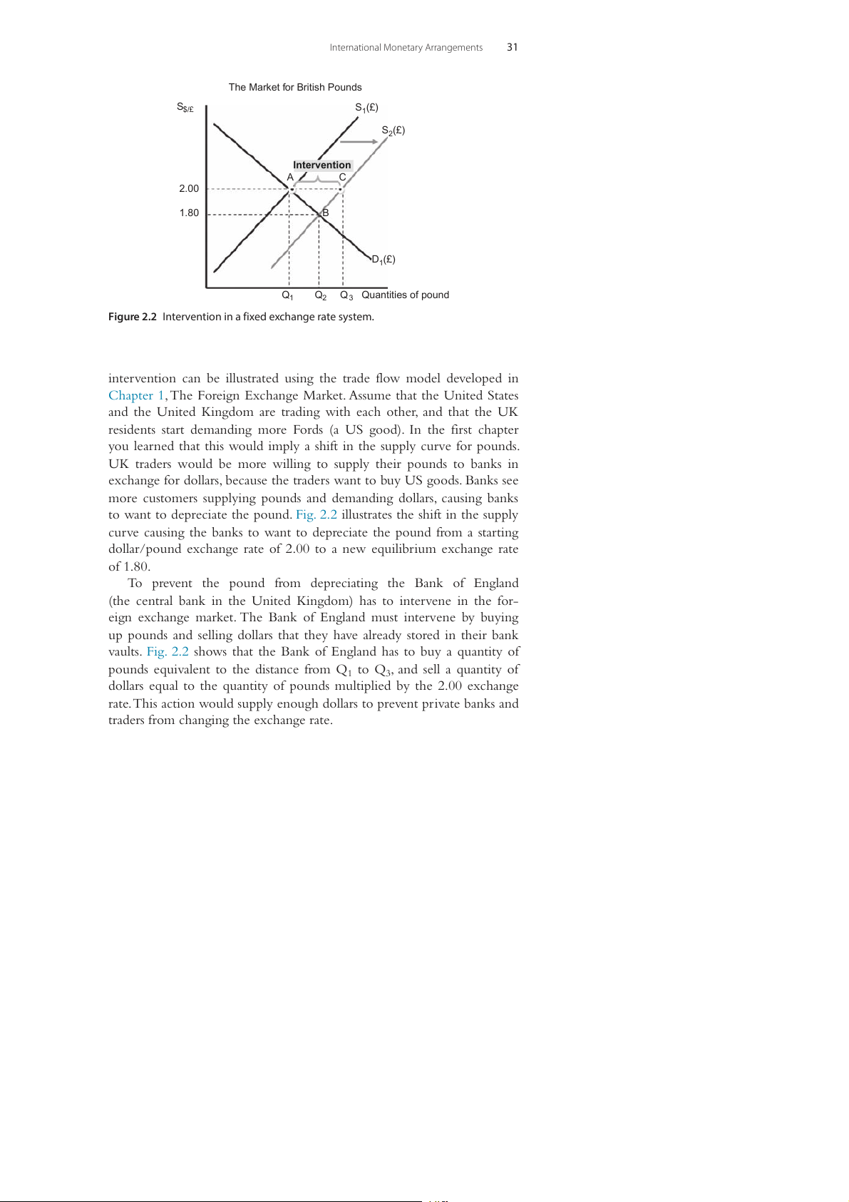
Figure 2.2 Intervention in a fixed exchange rate system.
intervention can be illustrated using the trade flow model developed in
Chapter1, The Foreign Exchange Market. Assume that the United States
and the United Kingdom are trading with each other, and that the UK
residents start demanding more Fords (a US good). In the first chapter
you learned that this would imply a shift in the supply curve for pounds.
UK traders would be more willing to supply their pounds to banks in
exchange for dollars, because the traders want to buy US goods. Banks see
more customers supplying pounds and demanding dollars, causing banks
to want to depreciate the pound. Fig. 2.2 illustrates the shift in the supply
curve causing the banks to want to depreciate the pound from a starting
dollar/pound exchange rate of 2.00 to a new equilibrium exchange rate of 1.80.
To prevent the pound from depreciating the Bank of England
(the central bank in the United Kingdom) has to intervene in the for-
eign exchange market. The Bank of England must intervene by buying
up pounds and selling dollars that they have already stored in their bank
vaults. Fig. 2.2 shows that the Bank of England has to buy a quantity of
pounds equivalent to the distance from Q to Q , and sell a quantity of 1 3
dollars equal to the quantity of pounds multiplied by the 2.00 exchange
rate. This action would supply enough dollars to prevent private banks and
traders from changing the exchange rate. 32
International Money and Finance
FAQ: What Are Special Drawing Rights?
There is one odd currency that is priced in any currency table, but does not physi-
cally exist, namely the Special Drawing Right (SDR). This “currency” was issued by
the IMF, but never existed in physical form. Instead it has been used as a unit of
account for a long time. For example, all of IMF’s own accounts are quoted in SDRs.
The SDR first appeared in 1969. The SDR was used to support the Bretton
Woods fixed exchange rate system. Participating countries in the Bretton Woods
agreement needed more official reserves to support the domestic exchange
rate. However, at that time, the supply of gold and US dollars was insufficient for
the rapid growth of world trade. The SDR provided more liquidity to the world
markets and allowed countries to continue to expand trade. The SDR does not
exist as notes and coins, but has value because all member countries of the IMF have agreed to accept it.
Allocations of SDRs are rare, and have only happened four times in his-
tory. The first allocation was in 1970–72 (SDR 9.3 billion) in the very end of the
Bretton Woods system. The next one was in 1979–81 (SDR 12.1 billion). After
that no more SDRs were allocated until the Great Recession. In August 28, 2009
SDR 161.2 billion were allocated and 21.5 billion SDRs were allocated shortly
thereafter in September 9, 2009. Further information about the SDRs can be
obtained from http://www.imf.org/external/np/exr/facts/sdr.HTM.
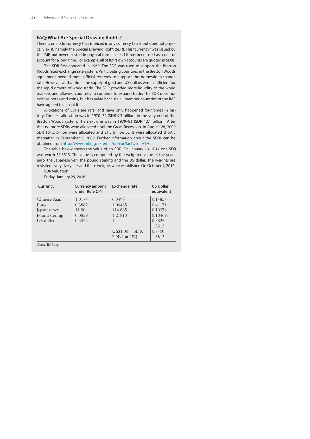
The table below shows the value of an SDR. On January 13, 2017 one SDR
was worth $1.3513. The value is computed by the weighted value of the yuan,
euro, the Japanese yen, the pound sterling and the US dollar. The weights are
revisited every five years and these weights were established On October 1, 2016. SDR Valuation Friday, January 29, 2016 Currency Currency amount Exchange rate US Dollar under Rule O-1 equivalent Chinese Yuan 1.0174 6.8490 0.14854 Euro 0.3867 1.06465 0.411711 Japanese yen 11.90 114.665 0.103781 Pound sterling 0.0859 1.21810 0.104691 US dollar 0.5825 1 0.5825 1.3513 US$1.00 = SDR 0.7400 SDR1 = US$ 1.3513 Source: IMF.org.
International Monetary Arrangements 33
Note that the model used to illustrate the intervention is a flow model.
This means that in each period the situation will occur. For example, if the
period is a year, then the excess supply of pounds will exist every year, as long
as the new demand for Fords exists. Thus, the Bank of England has to inter-
vene each year and buy pounds and sell dollars. If the excess supply persists
too long, the Bank of England may run out of dollars in their vaults, and
would be forced to apply for permission from the IMF to devalue their cur-
rency to be in line with the new market exchange rate (in this example 1.80).
THE BREAKDOWN OF THE BRETTON WOODS SYSTEM
The Bretton Woods system worked well through the 1950s and part of the
1960s. In 1960, there was a dollar crisis because the United States had run
large balance of payments deficits in the late 1950s. Concern over large
foreign holdings of dollars led to an increased demand for gold. Central
bank cooperation in an international gold pool managed to stabilize
gold prices at the official rate, but still the pressures mounted. Although
the problem of chronic US deficits and Japanese and European surpluses
could have been remedied by revaluing the undervalued yen, mark, and
franc, the surplus countries argued that it was the responsibility of the
United States to restore balance of payments equilibrium.
The failure to realign currency values in the face of fundamental eco-
nomic change spelled the beginning of the end for the gold exchange stan-
dard of the Bretton Woods agreement. By the late 1960s the foreign dollar
liabilities of the United States were much larger than the US gold stock.
The pressures of this “dollar glut” finally culminated in August 1971, when
President Nixon declared the dollar to be inconvertible and provided a close
to the Bretton Woods era of fixed exchange rates and convertible currencies.
THE TRANSITION YEARS: 1971–1973
In December 1971, an international monetary conference was held
to realign the foreign exchange values of the major currencies. The
Smithsonian agreement provided for a change in the dollar per gold
exchange value from $35 to $38.02 per ounce of gold. At the same time
that the dollar was being devalued by about 8%, the surplus countries saw
their currencies revalued upward. After the change in official currency
values the system was to operate with fixed exchange rates under which
the central banks would buy and sell their currencies to maintain the
exchange rate within 2.25% of the stated parity. Although the realignment 34
International Money and Finance
of currency values provided by the Smithsonian agreement allowed a
temporary respite from foreign exchange crises, the calm was short-lived.
Speculative flows of capital began to put downward pressure on the pound
and lira. In June 1972, the pound began to float according to supply and
demand conditions. The countries experiencing large inflows of specula-
tive capital, such as Germany and Switzerland, applied legal controls to
slow further movements of money into their countries.
Although the gold value of the dollar had been officially changed, the
dollar was still inconvertible into gold, and thus the major significance
of the dollar devaluation was with respect to the foreign exchange value of
the dollar, not to official gold movements. The speculative capital flows
of 1972 and early 1973 led to a further devaluation of the dollar in February
1973, when the official price of an ounce of gold rose from $38 to $42.22.
Still, the speculative capital flows persisted from the weak to the strong
currencies. Finally, in March 1973, the major currencies began to float.
INTERNATIONAL RESERVE CURRENCIES
International reserves are the means of settling international debts. Under
the gold standard, gold was the major component of international reserves.
Following World War II, we had a gold exchange standard in which inter-
national reserves included both gold and a reserve currency, the US dollar.
The reserve currency country was to hold gold as backing for the out-
standing balances of the currency held by foreigners. These foreign holders
of the currency were then free to convert the currency into gold if they
wished. However, as we observed with the dollar, once the convertibility
of the currency becomes suspect, or once large amounts of the currency
are presented for gold, the system tends to fall apart.
At the end of World War II, and throughout the 1950s, the world
demanded dollars for use as an international reserve. During this time,
US balance of payments deficits provided the world with a much-needed
source of growth for international reserves. As the rest of the world devel-
oped and matured, over time US liabilities to foreigners greatly exceeded
the gold reserve backing these liabilities. Yet as long as the increase in
demand for these dollar reserves equaled the supply, the lack of gold back-
ing was irrelevant. Through the late 1960s, US political and economic
events began to cause problems for the dollar’s international standing,
and the continuing US deficits were not matched by a growing demand,
so that pressure to convert dollars into gold resulted in the dollar being
declared officially no longer exchangeable for gold in August 1971.
International Monetary Arrangements 35
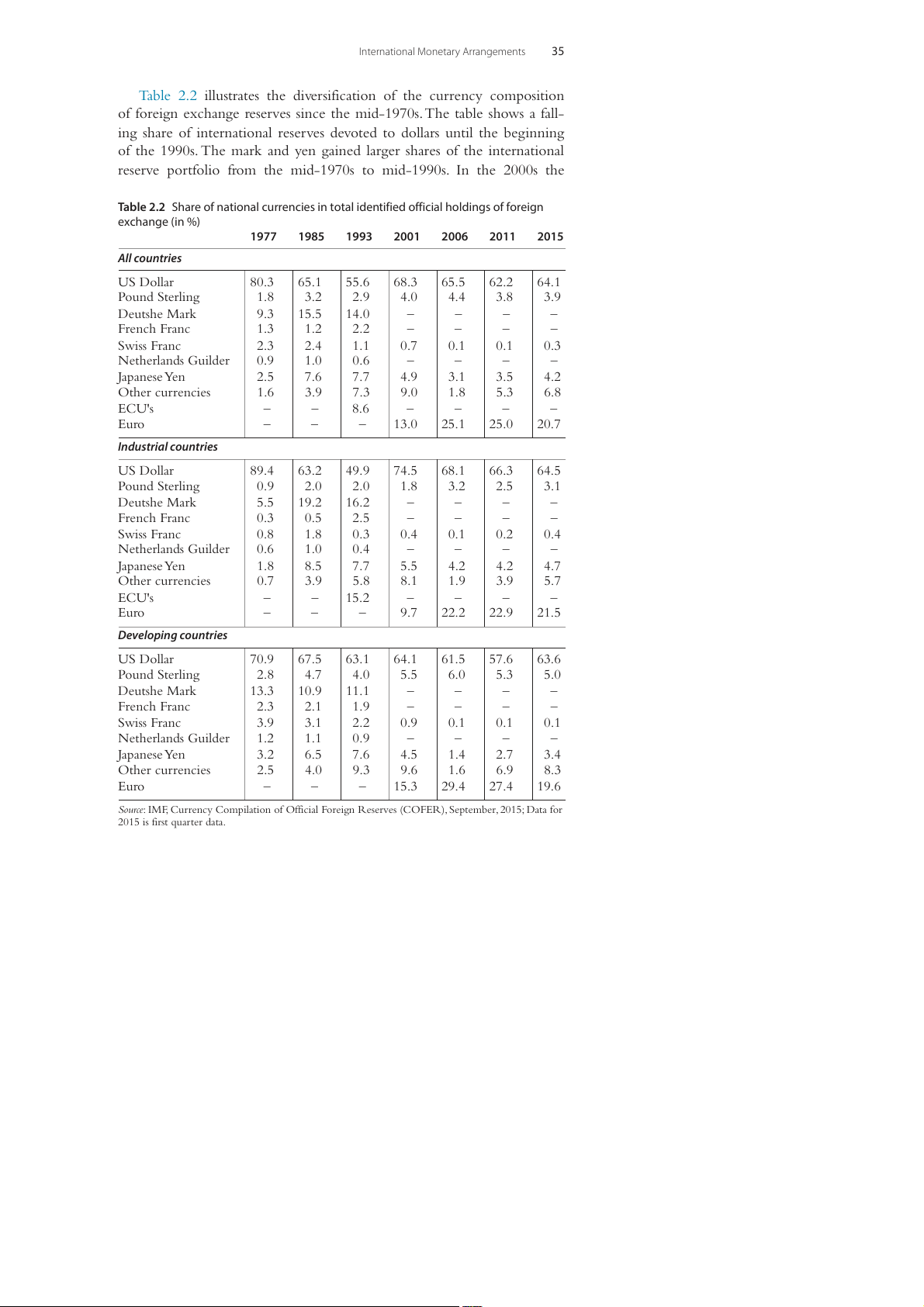
Table 2.2 illustrates the diversification of the currency composition
of foreign exchange reserves since the mid-1970s. The table shows a fall-
ing share of international reserves devoted to dollars until the beginning
of the 1990s. The mark and yen gained larger shares of the international
reserve portfolio from the mid-1970s to mid-1990s. In the 2000s the
Table 2.2 Share of national currencies in total identified official holdings of foreign exchange (in %) 1977 1985 1993 2001 2006 2011 2015 All countries US Dollar 80.3 65.1 55.6 68.3 65.5 62.2 64.1 Pound Sterling 1.8 3.2 2.9 4.0 4.4 3.8 3.9 Deutshe Mark 9.3 15.5 14.0 – – – – French Franc 1.3 1.2 2.2 – – – – Swiss Franc 2.3 2.4 1.1 0.7 0.1 0.1 0.3 Netherlands Guilder 0.9 1.0 0.6 – – – – Japanese Yen 2.5 7.6 7.7 4.9 3.1 3.5 4.2 Other currencies 1.6 3.9 7.3 9.0 1.8 5.3 6.8 ECU's – – 8.6 – – – – Euro – – – 13.0 25.1 25.0 20.7 Industrial countries US Dollar 89.4 63.2 49.9 74.5 68.1 66.3 64.5 Pound Sterling 0.9 2.0 2.0 1.8 3.2 2.5 3.1 Deutshe Mark 5.5 19.2 16.2 – – – – French Franc 0.3 0.5 2.5 – – – – Swiss Franc 0.8 1.8 0.3 0.4 0.1 0.2 0.4 Netherlands Guilder 0.6 1.0 0.4 – – – – Japanese Yen 1.8 8.5 7.7 5.5 4.2 4.2 4.7 Other currencies 0.7 3.9 5.8 8.1 1.9 3.9 5.7 ECU's – – 15.2 – – – – Euro – – – 9.7 22.2 22.9 21.5 Developing countries US Dollar 70.9 67.5 63.1 64.1 61.5 57.6 63.6 Pound Sterling 2.8 4.7 4.0 5.5 6.0 5.3 5.0 Deutshe Mark 13.3 10.9 11.1 – – – – French Franc 2.3 2.1 1.9 – – – – Swiss Franc 3.9 3.1 2.2 0.9 0.1 0.1 0.1 Netherlands Guilder 1.2 1.1 0.9 – – – – Japanese Yen 3.2 6.5 7.6 4.5 1.4 2.7 3.4 Other currencies 2.5 4.0 9.3 9.6 1.6 6.9 8.3 Euro – – – 15.3 29.4 27.4 19.6
Source: IMF, Currency Compilation of Official Foreign Reserves (COFER), September, 2015; Data for 2015 is first quarter data. 36
International Money and Finance
dollar share once again increased. Although the share of the dollar in 2015
is not as high as in the mid-1970s, it still exceeds 60% of the international
reserves. Furthermore, the euro has a substantial share of reserves, at 20.7%,
but it has not threatened the dominance of the dollar.
At first glance, it may appear very desirable to be the reserve currency and
have other countries accept your balance of payments deficits as a necessary
means of financing world trade. The difference between the cost of creating
new balances and the real resources acquired with the new balances is called
seigniorage. Seigniorage is a financial reward accruing to the issuer of currency.
The central bank’s seigniorage is the difference between the cost of money
creation and the return to the assets it acquires. In addition to such central
bank seigniorage, a reserve currency country also receives additional seignior-
age when foreign countries demand the currency issued and put those in its
vaults, as this reduces the inflationary pressure that money creation causes.
Table 2.2 indicates that the dollar is still, by far, the dominant reserve
currency. Since the US international position has been somewhat eroded
in the past few decades, the question arises as to why we did not see the
Japanese yen, or Swiss franc emerge as the dominant reserve currency.
Although the yen and Swiss franc have been popular currencies, the
respective governments in each country have resisted a greater interna-
tional role for their monies. Besides the apparently low additional sei-
gniorage return to the dominant international money, there is another
reason for these countries to resist. The dominant money producer (coun-
try) finds that international shifts in the demand for its money may have
repercussions on domestic operations. For a country the size of the United
States, domestic economic activity is large relative to international activity,
so international capital flows of any given magnitude have a much smaller
potential to disrupt US markets than would be the case for Japanese, or
Swiss markets, where foreign operations are much more important. In this
sense, it is clear why these countries have withstood the movement of the
yen and franc to reserve currency status. Over time, we may find that the
euro emerges as a dominant reserve currency as the combined economies
of the euro-area countries provide a very large base of economic activity.
However, Table 2.2 shows that the euro still only accounts for 20.7% of
total international reserves, so it is not close to the 64.1% share taken by
the dollar. In addition, the euro share seems to have stabilized at around
21–22% of the reserve holdings. Most of the growth in the euro reserve
holdings has come at the expense of other currencies than the dollar,
effectively creating a dual currency reserve system with the dollar and the
euro dominating the international reserves.
International Monetary Arrangements 37
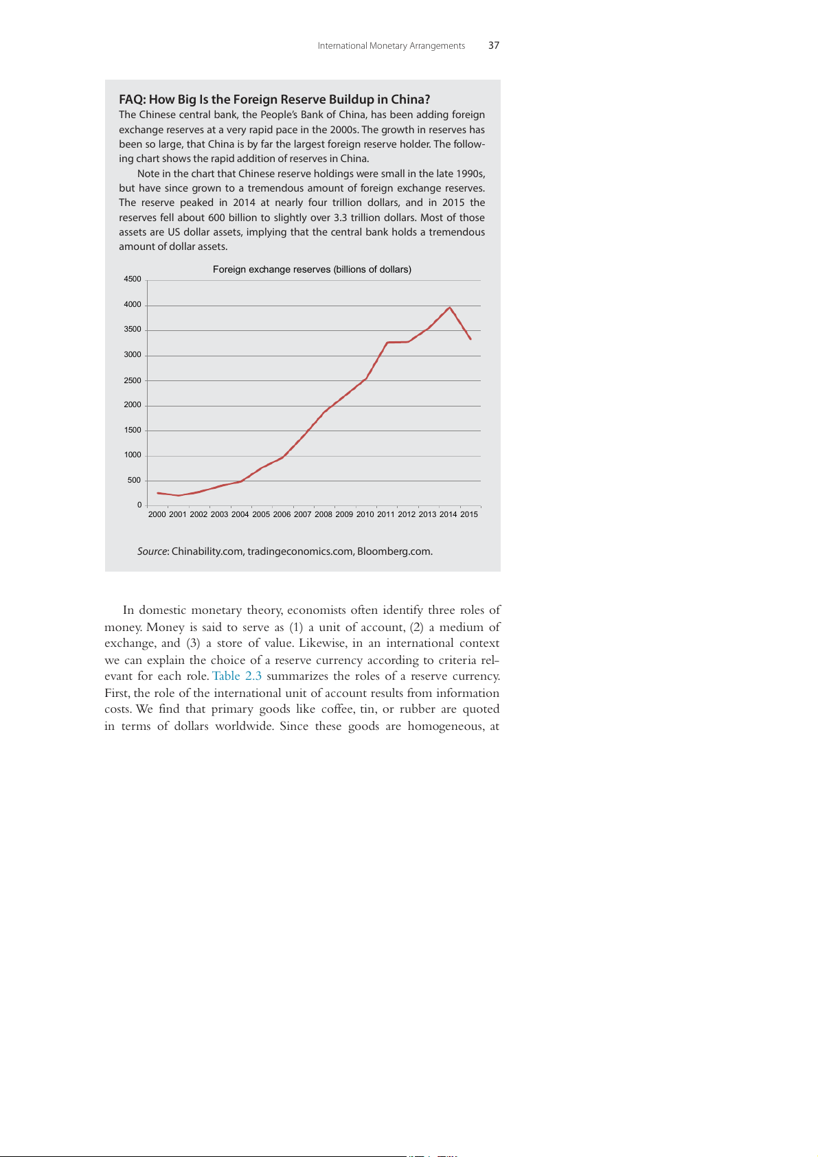
FAQ: How Big Is the Foreign Reserve Buildup in China?
The Chinese central bank, the People’s Bank of China, has been adding foreign
exchange reserves at a very rapid pace in the 2000s. The growth in reserves has
been so large, that China is by far the largest foreign reserve holder. The follow-
ing chart shows the rapid addition of reserves in China.
Note in the chart that Chinese reserve holdings were small in the late 1990s,
but have since grown to a tremendous amount of foreign exchange reserves.
The reserve peaked in 2014 at nearly four trillion dollars, and in 2015 the
reserves fell about 600 billion to slightly over 3.3 trillion dollars. Most of those
assets are US dollar assets, implying that the central bank holds a tremendous amount of dollar assets.
Foreign exchange reserves (billions of dollars) 4500 4000 3500 3000 2500 2000 1500 1000 500 0
2000 2001 2002 2003 2004 2005 2006 2007 2008 2009 2010 2011 2012 2013 2014 2015
Source: Chinability.com, tradingeconomics.com, Bloomberg.com.
In domestic monetary theory, economists often identify three roles of
money. Money is said to serve as (1) a unit of account, (2) a medium of
exchange, and (3) a store of value. Likewise, in an international context
we can explain the choice of a reserve currency according to criteria rel-
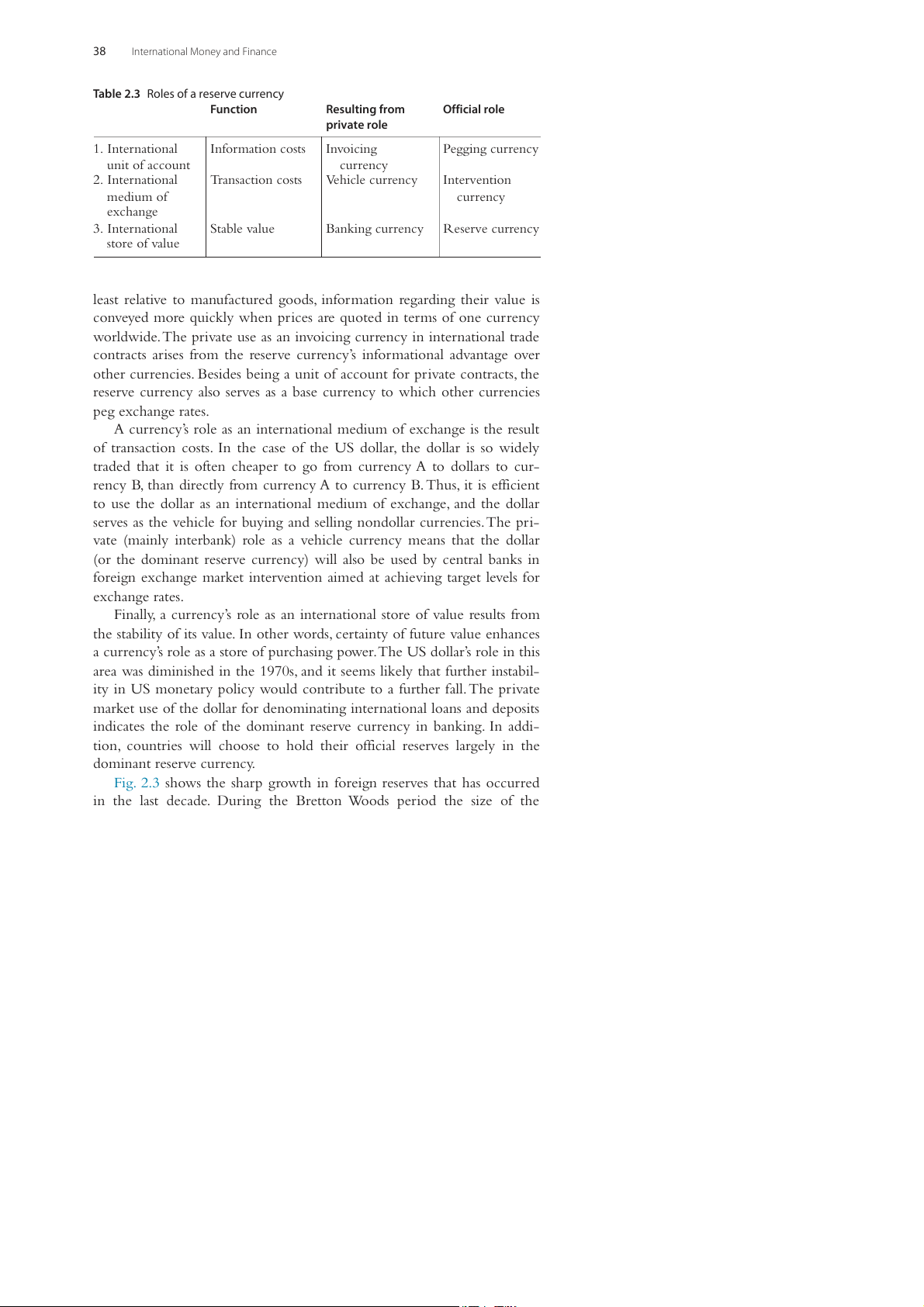
evant for each role. Table 2.3 summarizes the roles of a reserve currency.
First, the role of the international unit of account results from information
costs. We find that primary goods like coffee, tin, or rubber are quoted
in terms of dollars worldwide. Since these goods are homogeneous, at 38
International Money and Finance
Table 2.3 Roles of a reserve currency Function Resulting from Official role private role 1. International Information costs Invoicing Pegging currency unit of account currency 2. International Transaction costs Vehicle currency Intervention medium of currency exchange 3. International Stable value Banking currency Reserve currency store of value
least relative to manufactured goods, information regarding their value is
conveyed more quickly when prices are quoted in terms of one currency
worldwide. The private use as an invoicing currency in international trade
contracts arises from the reserve currency’s informational advantage over
other currencies. Besides being a unit of account for private contracts, the
reserve currency also serves as a base currency to which other currencies peg exchange rates.
A currency’s role as an international medium of exchange is the result
of transaction costs. In the case of the US dollar, the dollar is so widely
traded that it is often cheaper to go from currency A to dollars to cur-
rency B, than directly from currency A to currency B. Thus, it is efficient
to use the dollar as an international medium of exchange, and the dollar
serves as the vehicle for buying and selling nondollar currencies. The pri-
vate (mainly interbank) role as a vehicle currency means that the dollar
(or the dominant reserve currency) will also be used by central banks in
foreign exchange market intervention aimed at achieving target levels for exchange rates.
Finally, a currency’s role as an international store of value results from
the stability of its value. In other words, certainty of future value enhances
a currency’s role as a store of purchasing power. The US dollar’s role in this
area was diminished in the 1970s, and it seems likely that further instabil-
ity in US monetary policy would contribute to a further fall. The private
market use of the dollar for denominating international loans and deposits
indicates the role of the dominant reserve currency in banking. In addi-
tion, countries will choose to hold their official reserves largely in the dominant reserve currency.
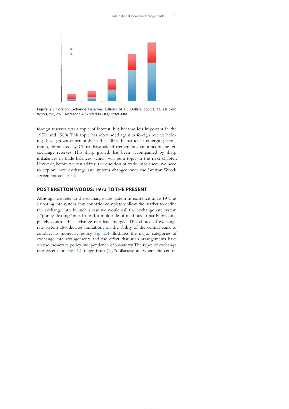
Fig. 2.3 shows the sharp growth in foreign reserves that has occurred
in the last decade. During the Bretton Woods period the size of the
International Monetary Arrangements 39 14000 12000 10000 Advanced markets 3928
Emerging and developing markets 8000 3092 6000 4000 7505 2078 6166 2000 1217 2240 932 458 719 0 1996 2000 2006 2010 2015
Figure 2.3 Foreign Exchange Reserves, Billions of US Dollars. Source: COFER Data
Report, IMF, 2015. Note that 2015 refers to 1st Quarter data.
foreign reserves was a topic of interest, but became less important in the
1970s and 1980s. This topic has rebounded again as foreign reserve hold-
ings have grown enormously in the 2000s. In particular emerging econ-
omies, dominated by China, have added tremendous amounts of foreign
exchange reserves. This sharp growth has been accompanied by sharp
imbalances in trade balances, which will be a topic in the next chapter.
However, before we can address the question of trade imbalances, we need
to explore how exchange rate systems changed once the Bretton Woods agreement collapsed.
POST BRETTON WOODS: 1973 TO THE PRESENT
Although we refer to the exchange rate system in existence since 1973 as
a floating rate system, few countries completely allow the market to define
the exchange rate. In such a case we would call the exchange rate system
a “purely floating” one. Instead, a multitude of methods to partly or com-
pletely control the exchange rate has emerged. This choice of exchange
rate system also dictates limitations on the ability of the central bank to
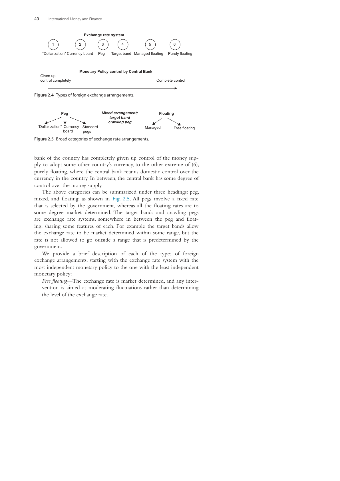
conduct its monetary policy. Fig. 2.4 illustrates the major categories of
exchange rate arrangements and the effect that such arrangements have
on the monetary policy independence of a country. The types of exchange
rate systems, in Fig. 2.4, range from (1), “dollarization” where the central 40
International Money and Finance Exchange rate system 1 2 3 4 5 6
“Dollarization” Currency board Peg Target band Managed floating Purely floating
Monetary Policy control by Central Bank Given up control completely Complete control
Figure 2.4 Types of foreign exchange arrangements. Peg
Mixed arrangement; Floating target band crawling peg
“Dollar ization” Currency Standard Managed Free floating board pegs
Figure 2.5 Broad categories of exchange rate arrangements.
bank of the country has completely given up control of the money sup-
ply to adopt some other country’s currency, to the other extreme of (6),
purely floating, where the central bank retains domestic control over the
currency in the country. In between, the central bank has some degree of control over the money supply.
The above categories can be summarized under three headings: peg,
mixed, and floating, as shown in Fig. 2.5. All pegs involve a fixed rate
that is selected by the government, whereas all the floating rates are to
some degree market determined. The target bands and crawling pegs
are exchange rate systems, somewhere in between the peg and float-
ing, sharing some features of each. For example the target bands allow
the exchange rate to be market determined within some range, but the
rate is not allowed to go outside a range that is predetermined by the government.
We provide a brief description of each of the types of foreign
exchange arrangements, starting with the exchange rate system with the
most independent monetary policy to the one with the least independent monetary policy:
Free floating—The exchange rate is market determined, and any inter-
vention is aimed at moderating fluctuations rather than determining
the level of the exchange rate.
International Monetary Arrangements 41
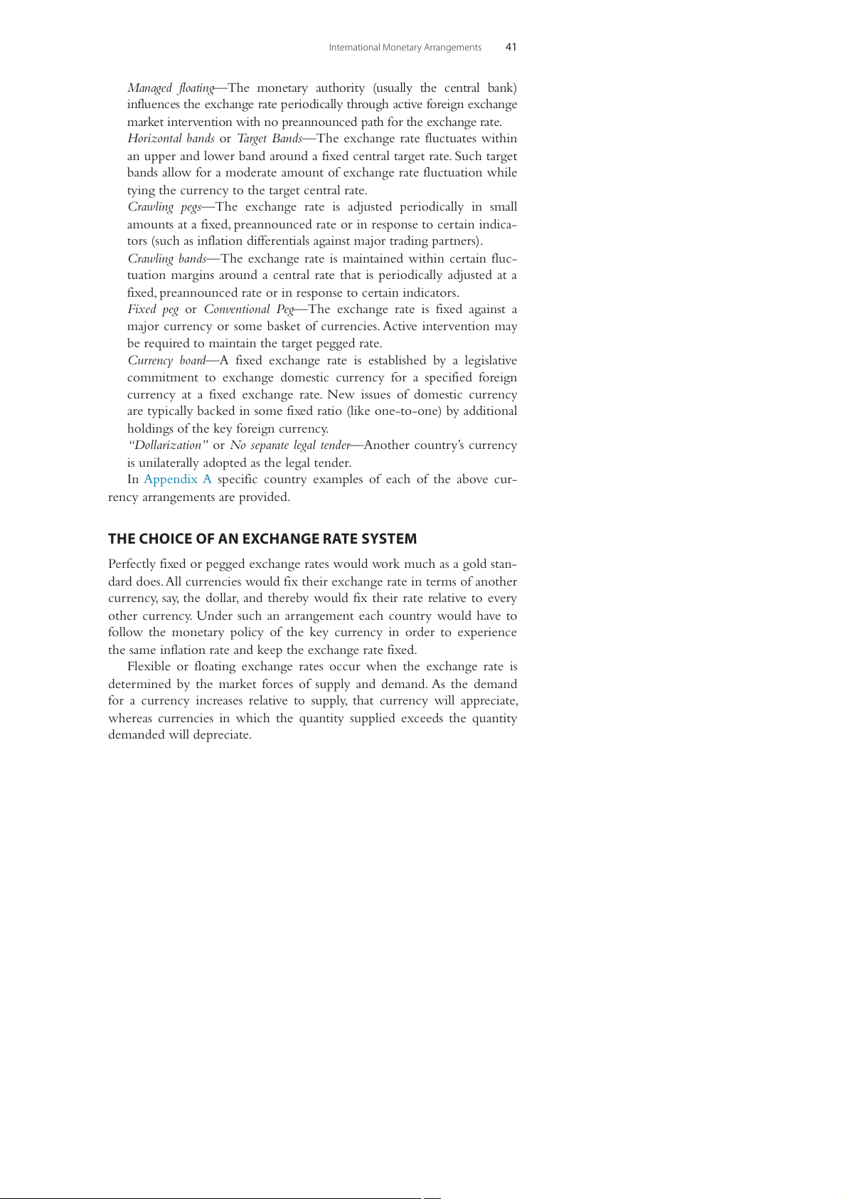
Managed floating—The monetary authority (usually the central bank)
influences the exchange rate periodically through active foreign exchange
market intervention with no preannounced path for the exchange rate.
Horizontal bands or Target Bands—The exchange rate fluctuates within
an upper and lower band around a fixed central target rate. Such target
bands allow for a moderate amount of exchange rate fluctuation while
tying the currency to the target central rate.
Crawling pegs—The exchange rate is adjusted periodically in small
amounts at a fixed, preannounced rate or in response to certain indica-
tors (such as inflation differentials against major trading partners).
Crawling bands—The exchange rate is maintained within certain fluc-
tuation margins around a central rate that is periodically adjusted at a
fixed, preannounced rate or in response to certain indicators.
Fixed peg or Conventional Peg—The exchange rate is fixed against a
major currency or some basket of currencies. Active intervention may
be required to maintain the target pegged rate.
Currency board—A fixed exchange rate is established by a legislative
commitment to exchange domestic currency for a specified foreign
currency at a fixed exchange rate. New issues of domestic currency
are typically backed in some fixed ratio (like one-to-one) by additional
holdings of the key foreign currency.
“Dollarization” or No separate legal tender—Another country’s currency
is unilaterally adopted as the legal tender.
In Appendix A specific country examples of each of the above cur-
rency arrangements are provided.
THE CHOICE OF AN EXCHANGE RATE SYSTEM
Perfectly fixed or pegged exchange rates would work much as a gold stan-
dard does. All currencies would fix their exchange rate in terms of another
currency, say, the dollar, and thereby would fix their rate relative to every
other currency. Under such an arrangement each country would have to
follow the monetary policy of the key currency in order to experience
the same inflation rate and keep the exchange rate fixed.
Flexible or floating exchange rates occur when the exchange rate is
determined by the market forces of supply and demand. As the demand
for a currency increases relative to supply, that currency will appreciate,
whereas currencies in which the quantity supplied exceeds the quantity demanded will depreciate. 42
International Money and Finance
Economists do not all agree on the advantages and disadvantages of a
floating as opposed to a pegged exchange rate system. For instance, some
would argue that a major advantage of flexible rates is that each coun-
try can follow domestic macroeconomic policies independent of the poli-
cies of other countries. To maintain fixed exchange rates, countries have
to share a common inflation experience, which was often a source of
problems under the post–World War II system of fixed exchange rates. If
the dollar, which was the key currency for the system, was inflating at a
rate faster than, say, Japan desired, then the lower inflation rate followed
by the Japanese led to pressure for an appreciation of the yen relative to
the dollar. Thus the existing pegged rate could not be maintained. Yet with
flexible rates, each country can choose a desired rate of inflation and the
exchange rate will adjust accordingly. Thus, if the United States chooses
8% inflation and Japan chooses 3%, there will be a steady depreciation of
the dollar relative to the yen (absent any relative price movements). Given
the different political environment and cultural heritage existing in each
country, it is reasonable to expect different countries to follow different
monetary policies. Floating exchange rates allow for an orderly adjustment
to these differing inflation rates.
Still there are those economists who argue that the ability of each
country to choose an inflation rate is an undesirable aspect of floating
exchange rates. These proponents of fixed rates indicate that fixed rates are
useful in providing an international discipline on the inflationary policies
of countries. Fixed rates provide an anchor for countries with inflationary
tendencies. By maintaining a fixed rate of exchange to the dollar (or some
other currency), each country’s inflation rate is “anchored” to the dollar,
and thus will follow the policy established for the dollar.
Critics of flexible exchange rates have also argued that flexible
exchange rates would be subject to destabilizing speculation. By destabi-
lizing speculation we mean that speculators in the foreign exchange mar-
ket will cause exchange rate fluctuations to be wider than they would be
in the absence of such speculation. The logic suggests that, if speculators
expect a currency to depreciate, they will take positions in the foreign
exchange market that will cause the depreciation as a sort of self-fulfilling
prophecy. But speculators should lose money when they guess wrong, so
that only successful speculators will remain in the market, and the suc-
cessful players serve a useful role by “evening out” swings in the exchange
rate. For instance, if we expect a currency to depreciate or decrease in
International Monetary Arrangements 43
value next month, we could sell the currency now, which would result
in a current depreciation. This will lead to a smaller future depreciation
than would occur otherwise. The speculator then spreads the exchange
rate change more evenly through time and tends to even out big jumps in
the exchange rate. If the speculator had bet on the future depreciation by
selling the currency now and the currency appreciates instead of depreci-
ates, then the speculator loses and will eventually be eliminated from the
market if such mistakes are repeated.
Research has shown that there are systematic differences between
countries choosing to peg their exchange rates and those choosing float-
ing rates. One very important characteristic is country size in terms of
economic activity or GDP. Large countries tend to be more independent
and less willing to subjugate domestic policies with a view toward main-
taining a fixed rate of exchange with foreign currencies. Since foreign
trade tends to constitute a smaller fraction of GDP the larger the country
is, it is perhaps understandable that larger countries are less attuned to for-
eign exchange rate concerns than are smaller countries.
The openness of the economy is another important factor. By open-
ness, we mean the degree to which the country depends on international
trade. The greater the fraction of tradable (i.e., internationally tradable)
goods in GDP, the more open the economy will be. A country with little
or no international trade is referred to as a closed economy. As previously
mentioned, openness is related to size. The more open the economy, the
greater the weight of tradable goods prices in the overall national price
level, and therefore the greater the impact of exchange rate changes on
the national price level. To minimize such foreign-related shocks to the
domestic price level, the more open economy tends to follow a pegged exchange rate.
Countries that choose higher rates of inflation than their trading
partners will have difficulty maintaining an exchange rate peg. We find,
in fact, that countries whose inflation experiences are different from the
average follow floating rates, or a crawling-peg-type system in which the
exchange rate is adjusted at short intervals to compensate for the inflation differentials.
Countries that trade largely with a single foreign country tend to
peg their exchange rate to that country’s currency. For instance, since the
United States accounts for the majority of Barbados trade, by pegging to
the US dollar, Barbados imparts to its exports and imports a degree of 44
International Money and Finance
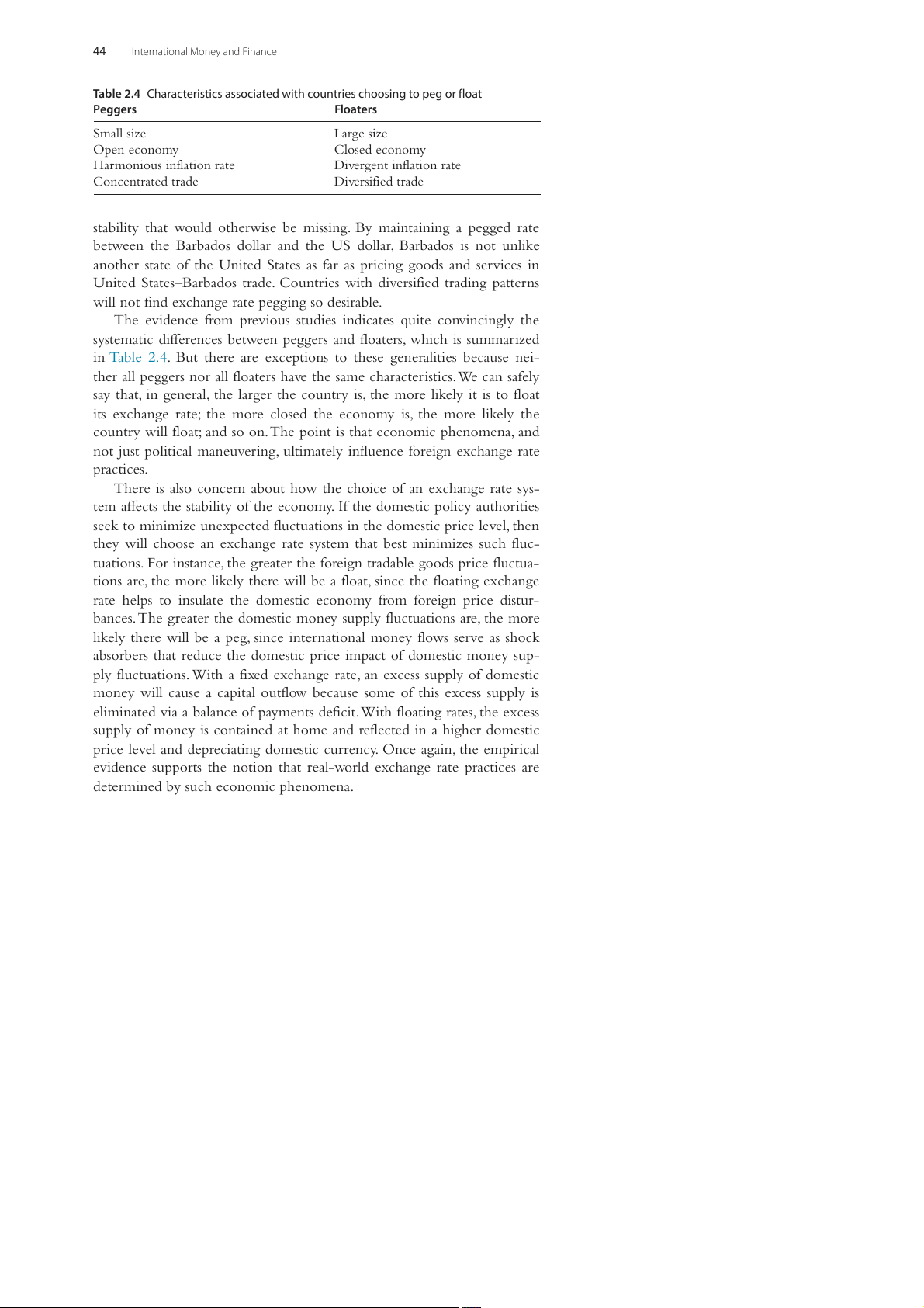
Table 2.4 Characteristics associated with countries choosing to peg or float Peggers Floaters Small size Large size Open economy Closed economy Harmonious inflation rate Divergent inflation rate Concentrated trade Diversified trade
stability that would otherwise be missing. By maintaining a pegged rate
between the Barbados dollar and the US dollar, Barbados is not unlike
another state of the United States as far as pricing goods and services in
United States–Barbados trade. Countries with diversified trading patterns
will not find exchange rate pegging so desirable.
The evidence from previous studies indicates quite convincingly the
systematic differences between peggers and floaters, which is summarized
in Table 2.4. But there are exceptions to these generalities because nei-
ther all peggers nor all floaters have the same characteristics. We can safely
say that, in general, the larger the country is, the more likely it is to float
its exchange rate; the more closed the economy is, the more likely the
country will float; and so on. The point is that economic phenomena, and
not just political maneuvering, ultimately influence foreign exchange rate practices.
There is also concern about how the choice of an exchange rate sys-
tem affects the stability of the economy. If the domestic policy authorities
seek to minimize unexpected fluctuations in the domestic price level, then
they will choose an exchange rate system that best minimizes such fluc-
tuations. For instance, the greater the foreign tradable goods price fluctua-
tions are, the more likely there will be a float, since the floating exchange
rate helps to insulate the domestic economy from foreign price distur-
bances. The greater the domestic money supply fluctuations are, the more
likely there will be a peg, since international money flows serve as shock
absorbers that reduce the domestic price impact of domestic money sup-
ply fluctuations. With a fixed exchange rate, an excess supply of domestic
money will cause a capital outflow because some of this excess supply is
eliminated via a balance of payments deficit. With floating rates, the excess
supply of money is contained at home and reflected in a higher domestic
price level and depreciating domestic currency. Once again, the empirical
evidence supports the notion that real-world exchange rate practices are
determined by such economic phenomena.
Tài liệu liên quan:
-

Hoạt động Tài chính của Doanh nghiệp Đa Quốc Gia (DN) - Chương 6 | Tài chính quốc tế | Trường Học Viện nông nghiệp Việt Nam
19 10 -
Hệ Thống Tiền Tệ Quốc Tế: Khái Niệm và Các Chế Độ Tỷ Giá | Tài chính quốc tế | Trường Học Viện nông nghiệp Việt Nam
24 12 -

Bài giảng Chương 1: Các Quan Hệ Cân Bằng Quốc Tế và LOP | Tài chính quốc tế | Trường Học Viện nông nghiệp Việt Nam
21 11 -
Cách Tính Lạm Phát và CPI: So Sánh Việt Nam và Mỹ | Tài chính quốc tế | Trường Học Viện nông nghiệp Việt Nam
23 12 -

Detailed Report and Analysis on Submission Trends | Tài chính quốc tế | Trường Học Viện nông nghiệp Việt Nam
23 12