Midterm review | Môn Inventory Management - Trường Đại học Quốc tế, Đại học Quốc gia Thành phố Hồ Chí Minh
Midterm review Môn Inventory Management. Tài liệu được sưu tầm gồm 12 trang, giúp bạn ôn tập tốt hơn. Mời các bạn đón xem.
Môn: Inventory Management 10 tài liệu
Trường: Trường Đại học Quốc tế, Đại học Quốc gia Thành phố Hồ Chí Minh 1.9 K tài liệu
Tác giả:


Preview text:
lOMoAR cPSD| 58605085 INVENTORY MANAGEMENT MIDTERM REVIEW Semester 1 – 2021 – 2022 Contents
INVENTORY MANAGEMENT .......................................................................................................................................................................................... 1
MIDTERM REVIEW ......................................................................................................................................................................................................... 1
Semester 1 – 2021 – 2022 ............................................................................................................................................................................................. 1
Chapter 2: Order quantity when demand is approximately level .............................................................................................................................. 2
I. Basic Order quantity EOQ................................................................................................................................................................................... 2
II. Quantity Discount ............................................................................................................................................................................................. 2
Chapter 3: Lot sizing for individual items with time varying demand....................................................................................................................... 3
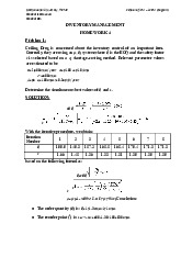
Chapter 4: Individual items with probabilistic demand ............................................................................................................................................. 6
I. Notation ................................................................................................................................................................................................................. 6
II. Procedure to find decision variables in given inventory policy ............................................................................................................................. 7
III. Formulars to find some interested outputs: ...................................................................................................................................................... 10
IV. Procedure to find random variable based on given distribution ....................................................................................................................... 11 lOMoAR cPSD| 58605085
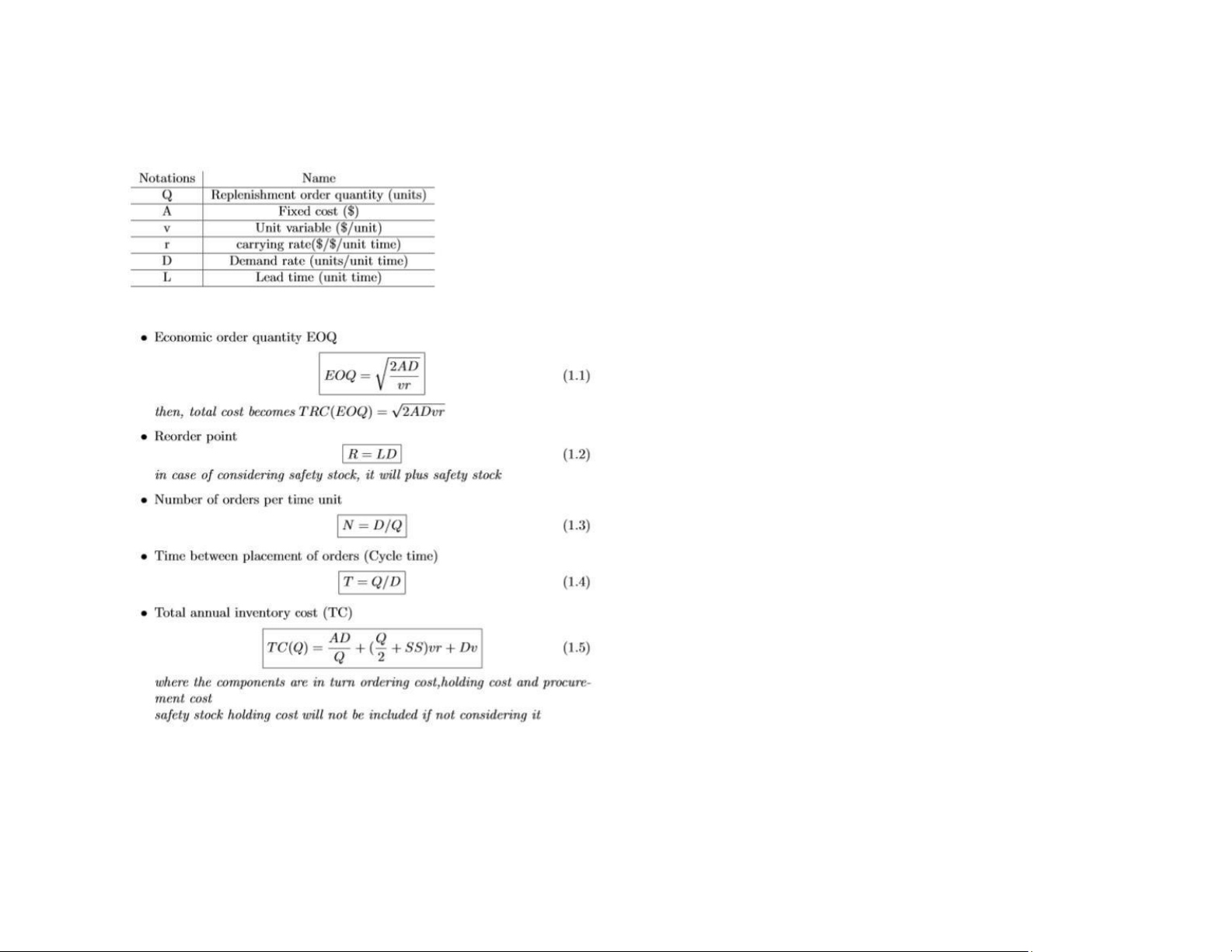
Chapter 2: Order quantity when demand is approximately level I. Basic Order quantity EOQ II. Quantity Discount
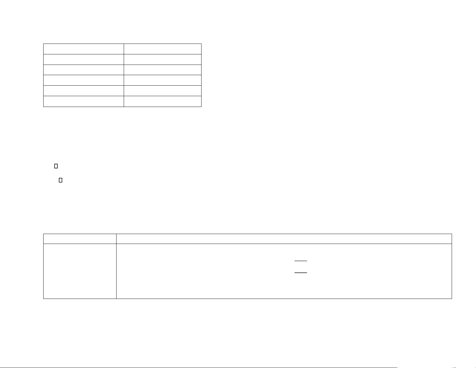
Given quantity schedule as follows: lOMoAR cPSD| 58605085 Order quantity Discounted price 1-299 $10.00 300-599 $9.75 600-999 $9.40 1000-4999 $9.50 5000 $9.00
Step 1: Find the optimal order Qi* for each discount level “i” by using the formula
Step 2: For each discount level “i” modify Qi* as follows If Q* < qi, then Qi* = qi.
If qi Q* < qi+1, then Qi* = Q*
If qi+1 Q*, eliminate this level from further consideration.
Step 3: Substitute the modified Qi* value in the total cost formula TC(Qi*).
Step 4: Select the Qi* that minimizes TC(Qi*)
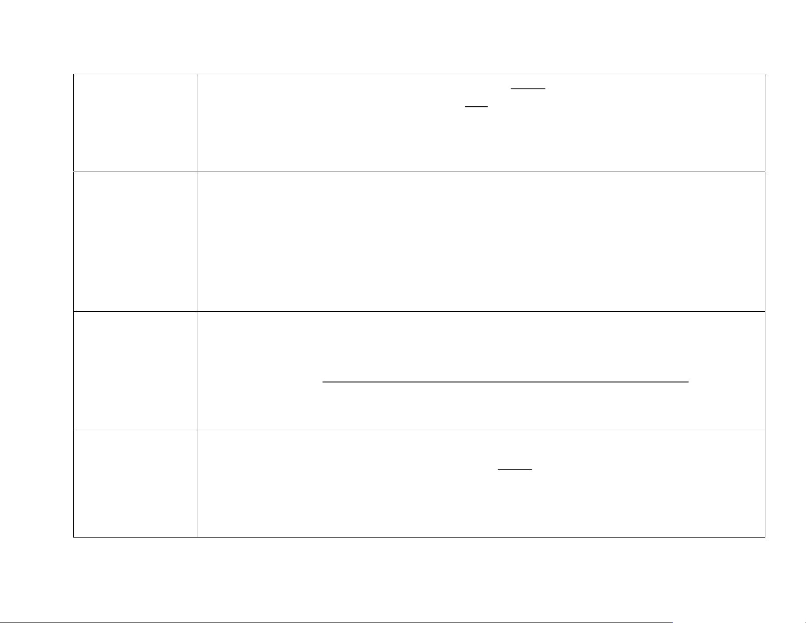
Chapter 3: Lot sizing for individual items with time varying demand Approach Method Fixed order quantity
Step1 : cumulate the requirement of period (FOQ)
Step2: Compare with EOQ, the nearest one to EOQ is the order replenishment quantity to the end of that period 2 𝐴𝐷 𝐸𝑂𝑄 = √ 𝑣𝑟 lOMoAR cPSD| 58605085 The economic order
Step1: calculate the fixed optimal time supply: quantity as time supply 𝐸𝑂𝑄 2𝐴 (POQ) 𝑇𝐸𝑂𝑄 = = √ 𝐷𝑎𝑣𝑔 𝐷𝑎𝑣𝑔𝑣𝑟
Round to the nearest integer that > 0
Step2: replenishment quantity must cover exactly the requirement of this integer number of periods 𝑅𝑜𝑢𝑛𝑑(𝑇𝐸𝑂𝑄) Wagner – Whitin
Suppose 𝐹(𝑡) as the total cost of the best replenishment that satisfies demand requirement in period 1,2, … , 𝑡 method
Then, 𝐹(1) = ∑𝑐𝑜𝑠𝑡 𝑟𝑒𝑝𝑙𝑒𝑛𝑖𝑠ℎ𝑚𝑒𝑛𝑡 𝑎𝑡 𝐽𝑎𝑛.
There are t options (order at month 𝑖 = 1,2,3, … 𝑡
Calculate ∑𝑐𝑜𝑠𝑡 𝑜𝑓 𝑜𝑝𝑡𝑖𝑜𝑛 𝑖 => the lowest one is 𝐹(𝑡)
Cách tính ∑𝑐𝑜𝑠𝑡
𝐸𝑥: 𝐹∗(1), 𝐹∗(2) are the min cost of replenishment that satisfies the demand requirement in period 1,2, … , 𝑡 𝐴
+ (𝐷2 + 2𝐷3)ℎ 𝑜𝑟𝑑𝑒𝑟 𝑎𝑡 1
𝐹∗(3) = min (𝐹∗(1) + 𝐴 + 𝐷3ℎ 𝑜𝑟𝑑𝑒𝑟 𝑎𝑡 2)
𝐹∗(2) + 𝐴 𝑜𝑟𝑑𝑒𝑟 𝑎𝑡 3 Silver – meal method
Selects the replenishment quantity that arrives at the beginning of the 1st period and cover to the end of 𝑖𝑡ℎ period Let
𝑇𝑅𝐶(𝑖) be the total relevant costs associated with a replenishment (1 𝑡𝑜 𝑖)
𝑇𝑅𝐶𝑈𝑇(𝑖) be the total relevant costs per unit time
𝑆𝑒𝑡𝑢𝑝 𝑐𝑜𝑠𝑡 (𝐴) + ∑𝑐𝑎𝑟𝑟𝑦𝑖𝑛𝑔 𝑐𝑜𝑠𝑡 𝑡𝑜 𝑡ℎ𝑒 𝑒𝑛𝑑 𝑜𝑓 𝑝𝑒𝑟𝑖𝑜𝑑 𝑖 + 𝑝𝑢𝑟𝑐ℎ𝑎𝑠𝑖𝑛𝑔 𝑐𝑜𝑠𝑡 𝑇𝑅𝐶(𝑖) = 𝑖 Cách tính carrying cost:
Ex: 𝐷1, 𝐷2, 𝐷3 are the demand for month 1,2, we want to calculate the carrying cost of ordering 1,2,3 at 1
𝐷2 ∗ ℎ ∗ (2 − 1) + 𝐷3 ∗ ℎ ∗ (3 − 1) 𝑇𝑅𝐶(𝑖) 𝑇𝑅𝐶𝑈𝑇 (𝑖) = 𝑖
Choose month 𝑖 in (1,2, … , 𝑇 − 1) that 𝑇𝑅𝐶𝑈𝑇(𝑖) < 𝑇𝑅𝐶𝑈𝑇(𝑖 + 1) for the first time Then, order quantity will be: 𝑖 lOMoAR cPSD| 58605085 𝑄 = ∑𝐷(𝑗) 𝑗=1 Least – Unit cost
The same procedure as Silver – meal but considering the least cost per unit (not per period) method (LUC) 𝑇𝑅𝐶(𝑖) 𝑇𝑅𝐶𝑈𝑇 Part – period balancing
Select the number of periods covered by the replenishment that ∑𝑐𝑎𝑟𝑟𝑦𝑖𝑛𝑔 𝑐𝑜𝑠𝑡𝑠 are made as close as 𝑠𝑒𝑡𝑢𝑝 𝑐𝑜𝑠𝑡 (𝐴) (PPB)
𝑐𝑎𝑟𝑟𝑦𝑖𝑛𝑔 𝑐𝑜𝑠𝑡 𝑎𝑡 𝑚𝑜𝑛𝑡ℎ 𝑖 + 1 = 𝑐𝑎𝑟𝑟𝑦𝑖𝑛𝑔 𝑐𝑜𝑠𝑡 𝑎𝑡 𝑚𝑜𝑛𝑡ℎ 𝑖 − 1 + (𝑖 − 1)𝐷(𝑖)𝑣𝑟 At
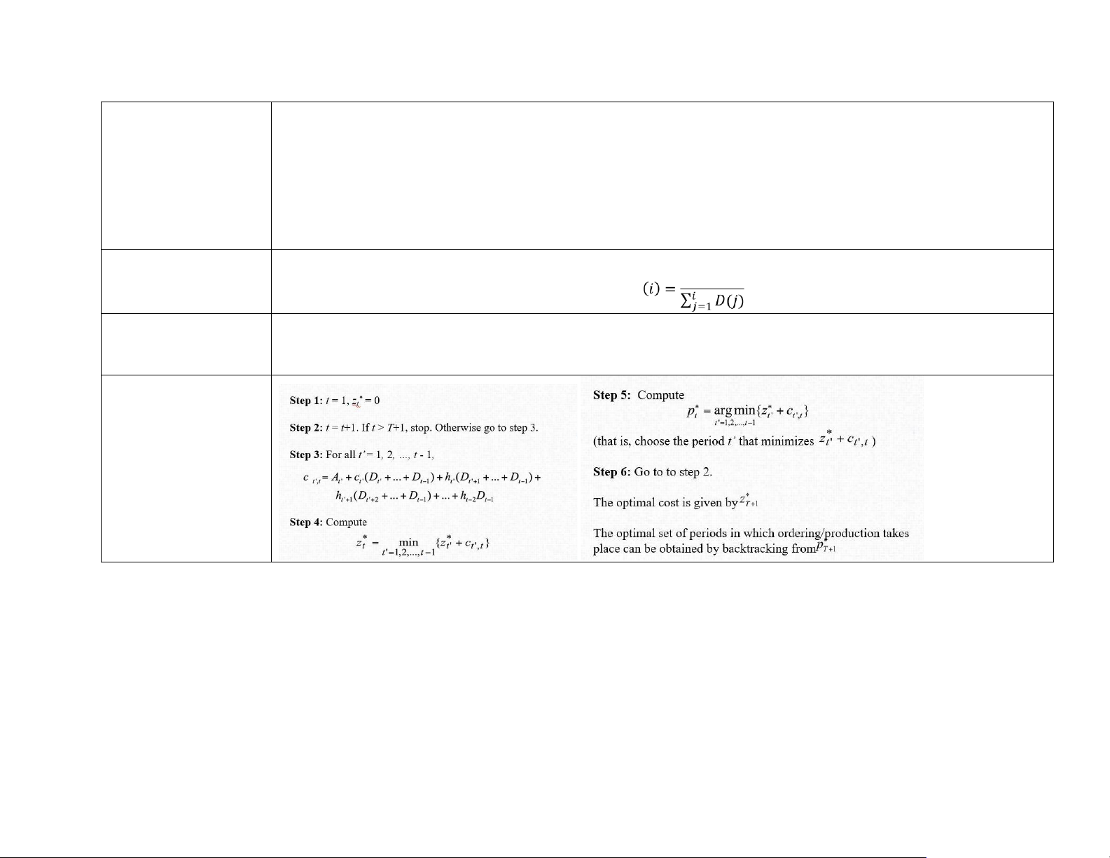
period 𝑖 that 𝑐𝑎𝑟𝑟𝑦𝑖𝑛𝑔 𝑐𝑜𝑠𝑡 < 𝐴, the first replenishment will cover requirement to the month 𝑖 Dynamic programming algorithm (network) lOMoAR cPSD| 58605085
Chapter 4: Individual items with probabilistic demand I. Notation Notation Meaning (unit) Notation Meaning (unit) 𝐴 Ordering cost ($/order) 𝑝
Stockout/penalty cost ($/unit) 𝑟 Carrying cost ($/$/time) 𝑔(𝑥)
Probability that demand during L is equal x 𝑣 Unit cost ($/unit) 𝐺(𝑥)
Probability that demand during L is ≤ x 𝐷 Demand rate (units/time) 𝐿(𝑧)
Special function of unit normal
distribution (table lookup), used
for finding 𝑛(𝑠) in case of normal distribution ℎ Holding cost ($/unit/time) 𝑛(𝑠) Expected number of stockouts per cycle 𝑏 Back-order cost ($/unit) 𝑄 Order quantity 𝐿 Lead time (time) 𝑠 Reorder point 𝑙 𝑎𝑛𝑑 𝜎𝐿
Mean and variance of lead time 𝑆 Order up to level distribution 𝜇 𝑎𝑛𝑑 𝜎2 Mean and variance of demand 𝑅 Review interval
distribution during lead time or time unit (if not having L) 𝛼 Service level (%) 𝛽 Fill rate (%) lOMoAR cPSD| 58605085 II.
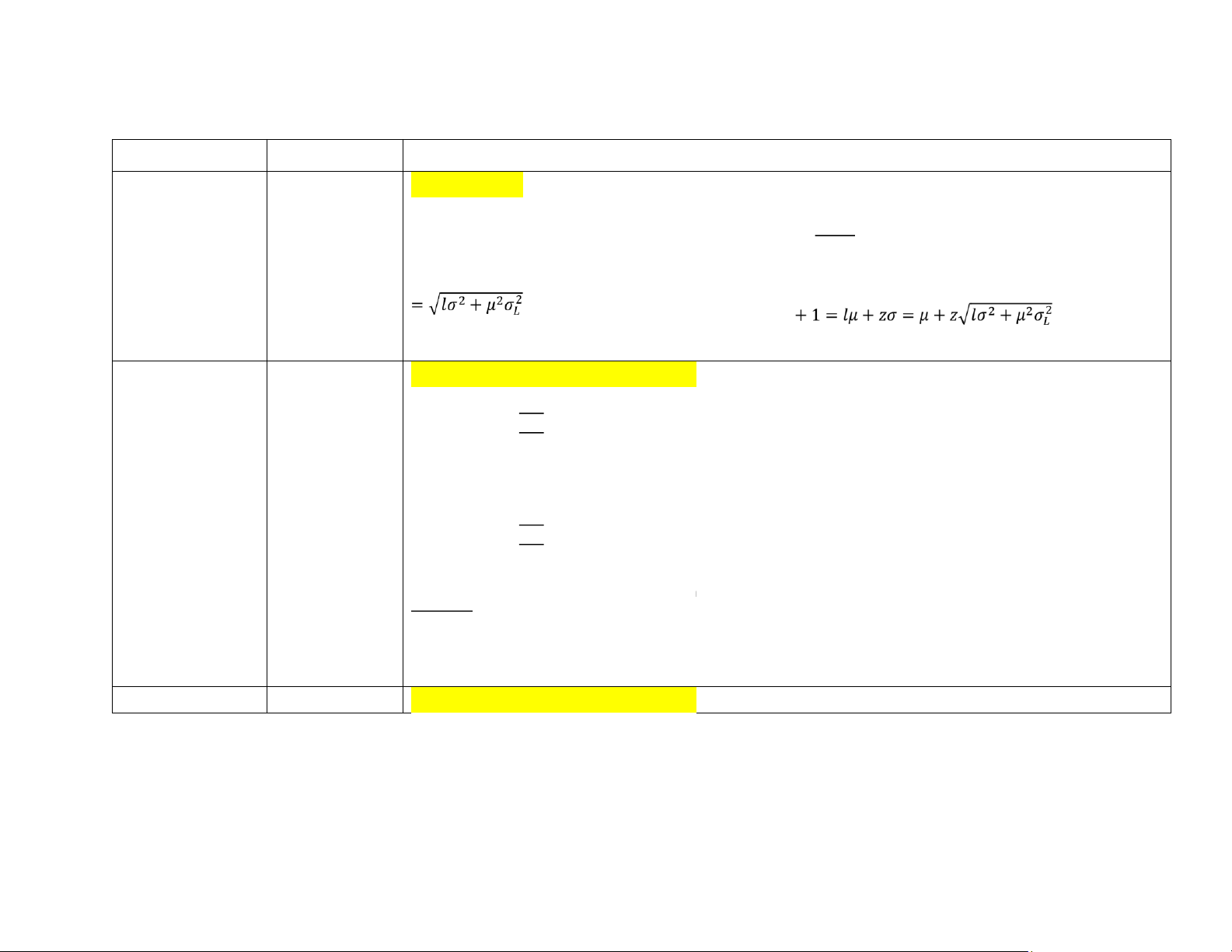
Procedure to find decision variables in given inventory policy Inventory policy Type of policy Decision variables Base stock Continuous Base stock 𝑠 ? (𝑠, 𝑠 + 1) model review 𝑏 𝐺(𝑠) = 𝑏 + ℎ
From the given distribution, we can find the associated value of base stock level 𝒔
When lead time is distributed with (𝑙, 𝜎𝐿2), then lead time demand std deviation becomes: Note: 𝜎
and base stock level becomes: 𝑠 Order quantity – Continuous
Order quantity 𝑄 and reorder point 𝑠 ?
Reorder point (𝑄, 𝑠) review
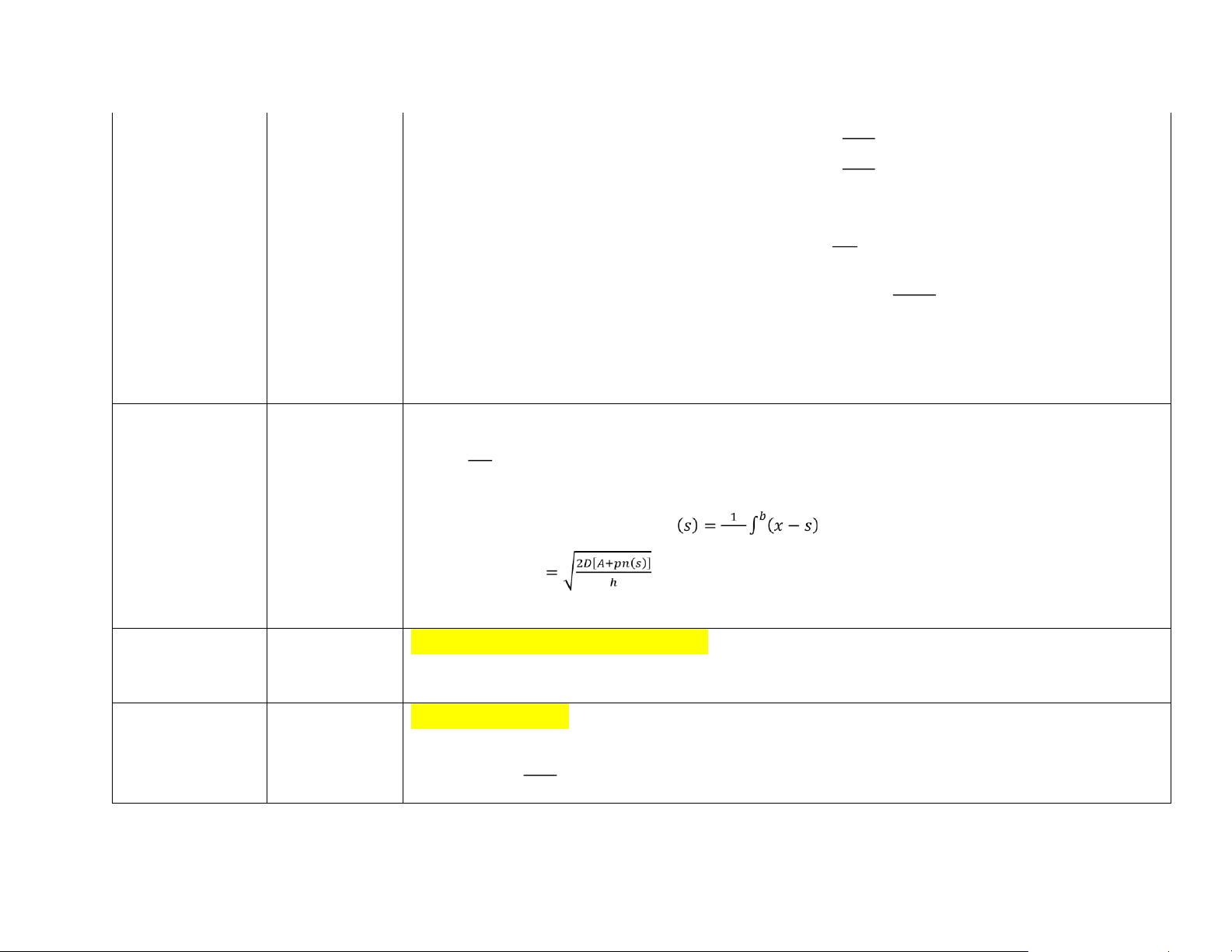
1. Given service level 𝜶 Type 1 given service 2 𝐴𝐷 level / fill rate 𝑄 = 𝐸𝑂𝑄 = √ ℎ
= 𝛼 and demand distribution => 𝑠
Find 𝑠: From given service level 𝐺(𝑠)
2. Given fill rate 𝜷 2 𝐴𝐷 𝑄 = 𝐸𝑂𝑄 = √ ℎ
Find 𝑠 step 1: calculate 𝐿(𝑧) = 𝐸𝑂𝑄hen look up normal probability and partial expression to find 𝑧 (1−𝛽) , t 𝜎
step 2: 𝑠 = 𝜇 + 𝑧 ∗ 𝜎
Order quantity 𝑄 and reorder point 𝑠 ? lOMoAR cPSD| 58605085 Order quantity – Continuous
Method 1: Sequential solution procedure (Approximation) Reorder point (𝑄, review 2 𝐴𝐷 𝑠) Type 2 given = √ 𝑄 = 𝐸𝑂𝑄 ℎ shortage cost Find 𝑠:
• in case of back-order cost consideration: 𝐺(𝑠) =
𝑏 => 𝑧 => 𝑠 = 𝜇 + 𝑧𝜎
• in case of shortage (stock out) cost 𝑏+ℎ consideration: 𝐺(𝑠) =
𝑝𝐷=> 𝑧 = > 𝑠 = 𝜇 + 𝑧𝜎
Method 2: Iterative solution procedure 𝑝𝐷+ℎ𝑄
Step 1: compute 𝑄 = 𝐸𝑂𝑄 (initial solution )
Step 2: Substitute 𝑄 to 𝐺(𝑠) = 1 − 𝑄 ℎ
𝑝𝐷 => Find out 𝑠 based on demand distribution
Step 3: Use 𝑠 to compute 𝑛(𝑠) = ∫𝑠∞ (𝑥 − 𝑠)𝑔(𝑥)𝑑𝑥 • For normal distribution: 𝑛(𝑠) = 𝜎𝐿(𝑧) where 𝑧 = 𝑠
−𝜇, 𝐿(𝑧) is obtained from looking up the 𝜎 normal
probability distribution and partial expectations
• For uniform distribution: 𝑛 𝑠 𝑑𝑥 𝑏−𝑎 Step 4: Solve for 𝑄
Step 5: Back to step 2 and continue until convergence (𝑠𝑖−1 = 𝑠𝑖 where 𝑖 is the current iteration)
Order up to level – Continuous
Order up to level 𝑆 and reorder point 𝑠 ?
Reorder point (𝑆, 𝑠) review
The procedure is as in (𝑄, 𝑠) model and set 𝑠 is
the same value, 𝑆 = 𝑠 + 𝑄 Periodic review –
Periodic review Order up to level 𝑆 ? Order up to level 𝑅 Given review interval (𝑅, 𝑆) 𝑅 Step 1: 𝐺(𝑆) = 𝑝
−ℎ , then based on the demand distribution to find 𝑆 𝑝 lOMoAR cPSD| 58605085 lOMoAR cPSD| 58605085 III.
Formulars to find some interested outputs:
Interested output (per time unit) Base stock model (approximation)
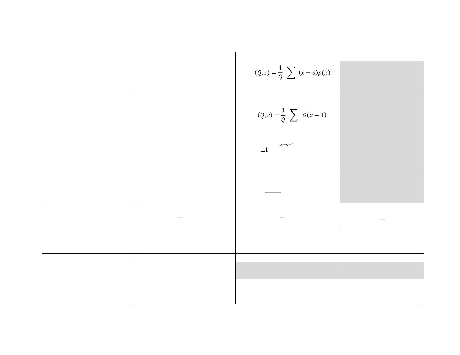
(𝑄, 𝑠) model and (𝑆, 𝑠) model (𝑅, 𝑆) model Expected back – order level
𝐵(𝑠) = 𝜇𝑝(𝑥) + (𝜇 − 𝑠)[1 − 𝐺(𝑠)] 𝑠+𝑄 𝐵 𝑥=𝑠+1 Approximation Expected service level
𝑆(𝑠) = 𝑃(𝑥 < 𝑠) = 𝐺(𝑠) Approximation 𝑠+𝑄 𝑆 = 1 − [𝐵(𝑠) − 𝐵(𝑠 + 𝑄)] 𝑄 Expected inventory level
𝐼(𝑠) = 𝑠 − 𝜇 + 𝐵(𝑠) Where Approximation:
𝜇 is mean demand per unit time 𝑄 + 1 𝐼(𝑄, 𝑠) =
+ 𝑠 − 𝐷𝐿 + 𝐵(𝑄, 𝑠) 2 Ordering cost per year 𝐷 𝐷 𝐴 ∗ 𝐴 ∗ 𝐴 𝑄 𝑄 𝑅 Holding cost per year
ℎ𝐼(𝑠) = ℎ[𝑠 − 𝜇 + 𝐵(𝑠)] 𝑄 𝐷𝑅
ℎ ∗ ( + 𝑠 − 𝐷𝐿) ℎ(𝑆 − 𝐷𝐿 − ) 2 2 Purchasing cost per year 𝐷 ∗ 𝑣 𝐷 ∗ 𝑣 𝐷 ∗ 𝑣 Back-order cost per year 𝑏 ∗ 𝐵(𝑠)
Where 𝑏 is backorder cost per unit Shortage cost per year 𝑘 ∗ 𝐵(𝑠) 𝑝𝐷𝑛(𝑠) 𝑝𝑛(𝑆)
Where 𝑘 is shortage cost per unit 𝑄 𝑅 lOMoAR cPSD| 58605085 Expected total cost per year
Holding cost + ordering cost + purchasing cost + back-order or shortage cost IV.
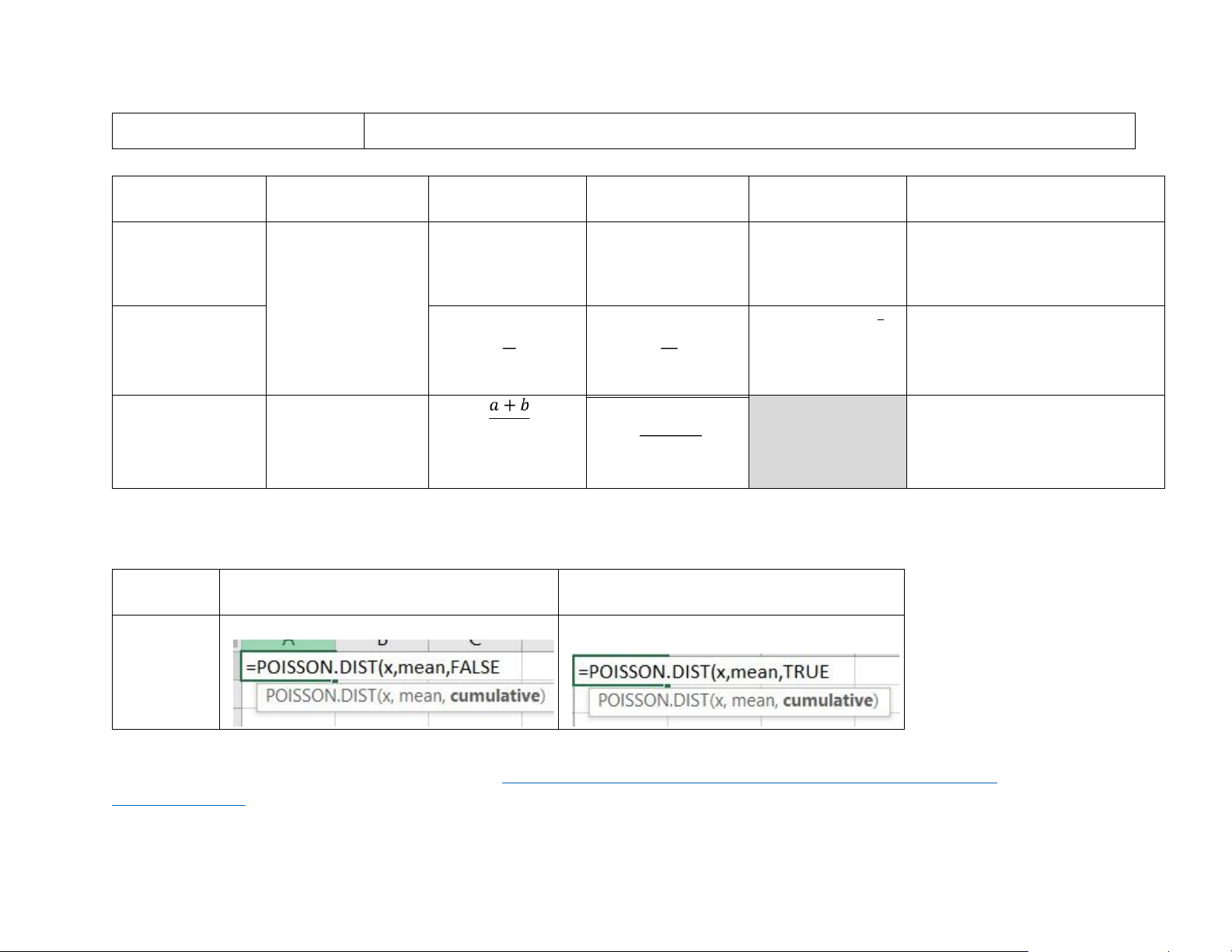
Procedure to find random variable based on given distribution Continuous Random variable Mean Variance 𝑐𝑑𝑓 𝐺(𝑥) 𝑥 Distribution Normal 𝑥 𝜇 𝜎2 Not used, use
Given service level 𝛼 => 𝑧𝛼 (It can be reorder standard normal point, order distribution instead
𝑥 = 𝜎𝑧𝛼 + 𝜇 quantity,…) Exponential (Time 1 1 𝑥
Given service level 𝐺(𝑥) = 𝛼 between
𝐺(𝑥) = 1 − 𝑒−𝜆 arrivals) 𝜆 𝜆2
𝑥 = −(𝜆)log (1 − 𝛼) (Time unit/units) Uniform (𝑏 − 𝑎)2
Given service level 𝐺(𝑥) = 𝛼 distribution ( 2 √ Demand is in the 12
𝑥 = 𝛼(𝑏 − 𝑎) interval [𝑎, 𝑏])
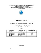
For discrete distribution such as Discrete, Poisson, Geometric distribution, we must establish a table by spreadsheet (take much effort to calculate by hand) as follow: Variable 𝑝𝑑𝑓 𝑔(𝑥) 𝑐𝑑𝑓 𝐺(𝑥) value 𝑥 Poisson (Number of occurrences per time unit)
Then, from the given 𝐺(𝑥) we can look up the table and find the interested value 𝑥
Source for more info about Probability and Distribution: https://openstax.org/books/introductory-business-statistics/pages/4-4- poissondistribution lOMoAR cPSD| 58605085
Tài liệu liên quan:
-
Project report template | Môn Inventory Management - Trường Đại học Quốc tế, Đại học Quốc gia Thành phố Hồ Chí Minh
109 55 -
Homework 6 Môn Inventory Management | Trường Đại học Quốc tế, Đại học Quốc gia Thành phố Hồ Chí Minh
136 68 -
Homework 5 Môn Inventory Management | Trường Đại học Quốc tế, Đại học Quốc gia Thành phố Hồ Chí Minh
146 73 -
Homework 4 Solutions: Problems 1, 2 & 3 | Môn Inventory Management - Trường Đại học Quốc tế, Đại học Quốc gia Thành phố Hồ Chí Minh
130 65 -
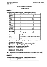
Homework 2 Môn Inventory Management | Trường Đại học Quốc tế, Đại học Quốc gia Thành phố Hồ Chí Minh
158 79