Notes: Key Concepts and Techniques | Môn Data Mining - Trường Đại học Quốc tế, Đại học Quốc gia Thành phố Hồ Chí Minh

lOMoAR cPSD| 23136115 Data mining
Chapter 1: Intro to data-mining What is data-mining
Def: The process of discovering patterns in data.
• The process must be automatic or semiautomatic.
• Patterns discovered must be meaningful in that they lead to some advantage, usually an economic one.
• The data is invariably presented in substantial quantities
The process of analyzing data from different perspectives and summarizing it into
useful information - information that can be used to increase revenue, cut costs, or both.
Example: Web usage mining.Given: click streams. Problem: prediction of user
behaviour. Data: historical records of embryos and outcome
Alternative name: Knowledge discovery (mining) in databases (KDD), knowledge
extraction, data/pattern analysis, data archeology, data dredging, information
harvesting, business intelligence, etc. Data mining Goals
DM is to extract information from a data set and transforming it into an understandable structure for further use.
-> Ultimate goal: PREDICTION.
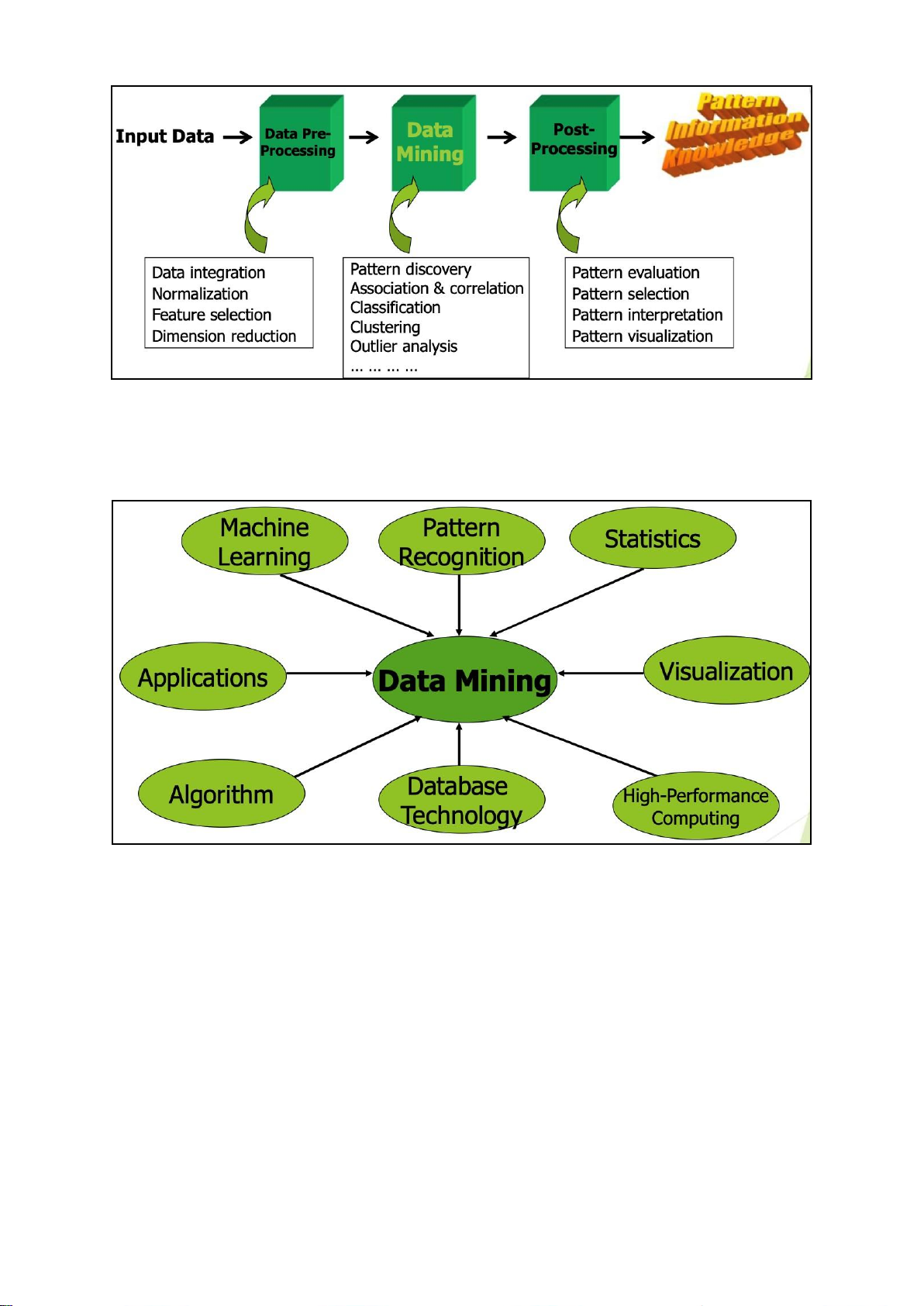
Stage of Data-mining process
1-Data cleaning -> 2-Data integration from multiple sources -> 4-Warehousing the
data -> 5-Data cube construction -> 6-Data selection for data mining -> 7-Data mining
-> 8-Presentation of the mining results -> 9-Patterns and knowledge to be used or stored into knowledge-base. lOMoAR cPSD| 23136115 Data Mining Techniques
CONFLUENCE OF MULTIPLE DISCIPLINES
WHY Confluence of multiple discipline ? - due to 4 factor 1. Tremendous amount of data
• Algorithms must be scalable to handle big data
2. High-dimensionality of data
• Micro-array may have tens of thousands of dimensions 3. High complexity of data
• Data streams and sensor data lOMoAR cPSD| 23136115
• Time-series data, temporal data, sequence data
• Structure data, graphs, social and information networks Spatial,
spatiotemporal, multimedia, text and Web data
• Software programs, scientific simulations
4. New and sophisticated applications
Machine learning techniques
• Structural descriptions represent patterns explicitly
• Can be used to predict outcome in new situation
• Can be used to understand and explain how prediction is derived
• Methods originate from artificial intelligence, statistics, and research on databases
Knowledge Representation Method 1. Tables 2. Data cube 3. Linear models 4. Trees 5. Rules
6. Instance-based Representation 7. Cluster IF-Then Rules :
If tear production rate = reduced then recommendation = none
Otherwise, if age = young and astigmatic = no then recommendation = soft Application
The result of learning—or the learning method itself— is deployed in practical applications
• Processing loan applications
• Screening images for oil slicks
• Electricity supply forecasting
• Diagnosis of machine faults lOMoAR cPSD| 23136115 • Marketing and sales
• Separating crude oil and natural gas
• Reducing banding in rotogravure printing
• Finding appropriate technicians for telephone faults
• Scientific applications: biology, astronomy, chemistry
• Automatic selection of TV programs
• Monitoring intensive care patients
Chapter 2: Getting to know your data Type of Data Sets 1 - Record 3 - Ordered • Relational records
• Video data: sequence of images
• Data matrix, e.g., numerical matrix,
• Temporal data: time-series crosstabs
• Sequential Data: transaction
• Document data: text documents: term- sequences
frequency vector • Transaction data • Genetic sequence data 2 - Graph and network
4 - Spatial, image and multimedia: • World Wide Web • Spatial data: maps
• Social or information networks • Image data: • Molecular Structures • Video data:
Important Characteristics of Structured Data 1 - Dimensionality • Curse of dimensionality 3 - Resolution 2 - Sparsity
• Patterns depend on the scale • Only presence counts 4 - Distribution • Centrality and dispersion Data Objects
Def: represent an entity can be called as samples , examples, instances, data points,
objects, tuples. Are describe by Atributes.
• Example: sales database: customers, store items, sales ; medical database:
patients, treatments ; university database: students, professors, courses Atributes
Also know as Dimension, Feature, Variables : data field, representing a characteristic or feature of a data object. lOMoAR cPSD| 23136115
• Example: customer_ID, name, address. Attribute Types:
1. Nominal - categories, states, or “names of things”
• Example: Hair_color = {auburn, black, blond, brown, grey, red, white} ; marital
status, occupation, ID numbers, zip codes
2. Binary - Nominal attribute with only 2 states (0 and 1)
1. Symmetric Binary - both outcomes equally important • Example: gender
2. Asymmetric Binary - outcomes not equally important.
• Example : medical test (positive vs. negative)
3. Ordinal - Values have a meaningful order (ranking) but magnitude between
successive values is not known.
• Example: Size = {small, medium, large}, grades, army rankings
4. Numeric - quantitative (integer / real-valued)
1. Interval-scaled - Measured on a scale of equal-sized units and value have order
and have no true zero-point.
• Example: temperature in C ̊or F ̊, calendar dates
2. Ratio-scaled - Inherent zero-point, we can speak of values as being an order
of magnitude larger than the unit of measurement (10 K ̊ is twice as high as 5 K ̊).
• Example: temperature in Kelvin, length, counts, monetary quantities.
Discrete vs Continuous Attributes
Discrete Att. - Has only a finite or countably infinite set of values, sometimes
represented as integer variables (Notes: Binary attributes are a special case of discrete attributes)
• Example: zip codes, profession, or the set of words in a collection of documents.
Continuous Att. - Has real numbers as attribute values, practically, real values can
only be measured and represented using a finite number of digits continuous attributes
are typically represented as floating-point variables.
• Example: temperature, height, or weight. lOMoAR cPSD| 23136115
Basic Statistical Description of Data
Motivation - To better understand the data: central tendency, variation and spread.
Data dispersion characteristics - median, max, min, quantiles, outliers, variance, etc.
Numerical dimensions correspond to sorted intervals
• Data dispersion: analyzed with multiple granularities of precision
• Boxplot or quantile analysis on sorted intervals
Dispersion analysis on computed measures - Folding measures into numerical
dimensions, boxplot or quantile analysis on the transformed cube.
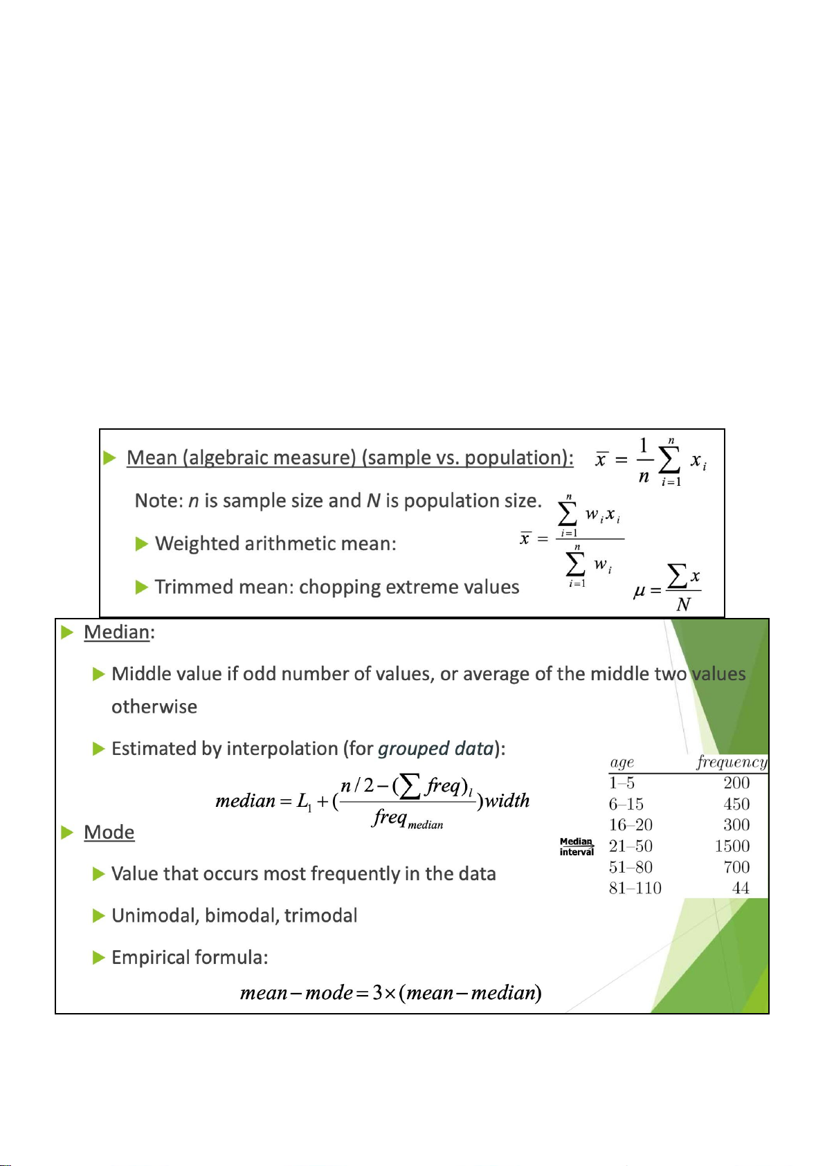
Measuring the Central tendency lOMoAR cPSD| 23136115
Measuring the Dispersion of Data
Quartiles, outliers and boxplots
• Quartiles: Q1 (25th percentile), Q3 (75th percentile)
• Inter-quartile range: IQR = Q3 − Q1
• Five number summary: min, Q1, median, Q3, max
• Boxplot: ends of the box are the quartiles; median is marked; add whiskers, and plot outliers individually
• Outlier: usually, a value higher/lower than 1.5 x IQR beyond the quartiles.
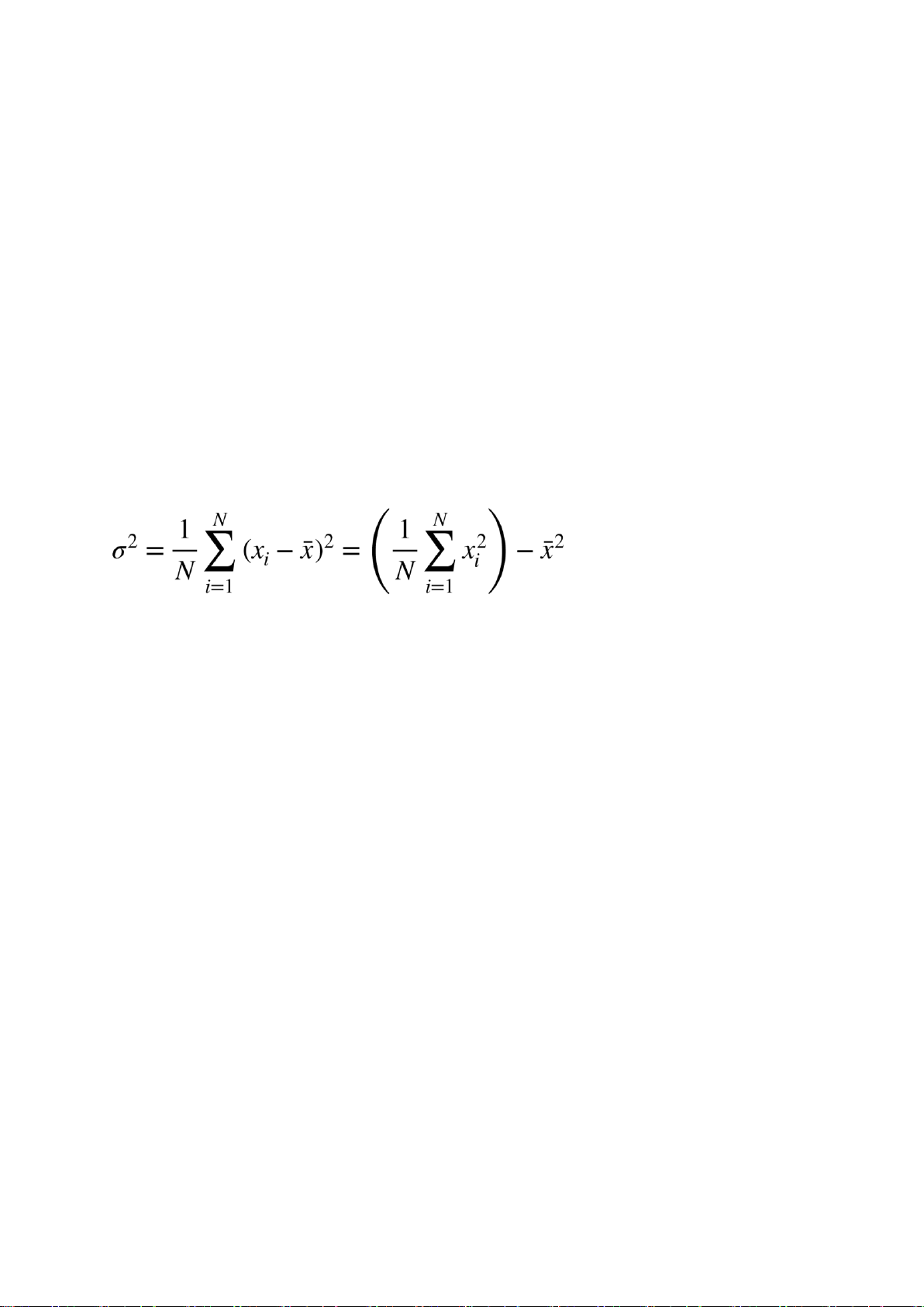
Variance and standard deviation (σ)
• Variance: (algebraic, scalable computation)
• Standard deviation σ is the square root of variance σ2 BoxPlot Analysis
Def : Data is represented with a box
• The ends of the box are at the first and third quartiles, i.e., the height of the box is IQR
• The median is marked by a line within the box
• Whiskers: two lines outside the box extended to Minimum and Maximum
• Outliers: points beyond a specified outlier threshold, plotted individually
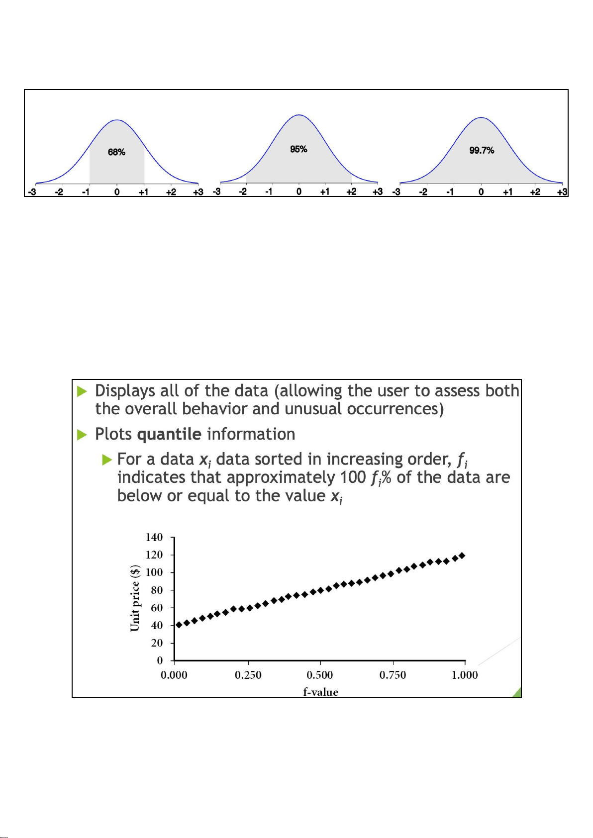
Properties of Normal Distribution Curve
The normal (distribution) curve
• From μ–σ to μ+σ: contains about 68% of the measurements (μ: mean, σ: standard deviation)
• From μ–2σ to μ+2σ : contains about 95% of it lOMoAR cPSD| 23136115
• From μ –3 σ to μ +3 σ : contains about 99.7% of it Histogram Analysis
Def : Graph display of tabulated frequencies, shown as bars. Shows what proportion
of cases fall into each of several categories. Differs from a bar chart in that it is the
area of the bar that denotes the value, not the height as in bar charts, a crucial
distinction when the categories are not of uniform width. The categories are usually
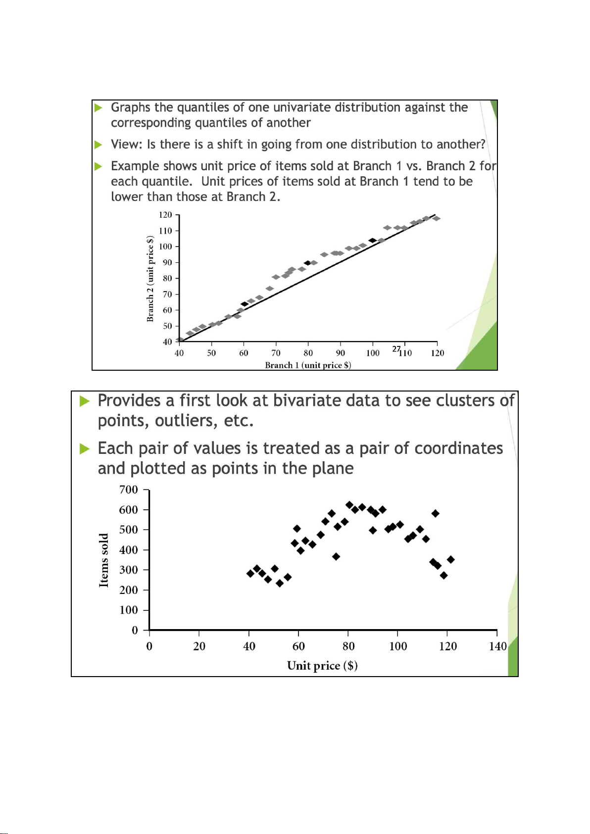
specified as non-overlapping intervals of some variable. The categories (bars) must be adjacent Quantile Plot lOMoAR cPSD| 23136115
Quantile-Quantile (Q-Q) Plot Scatter Plot
Similarity and Dissimilarity Similarity lOMoAR cPSD| 23136115
• Numerical measure of how alike two data objects are
• Value is higher when objects are more alike
• Often falls in the range [0,1]
Dissimilarity (e.g., distance)
• Numerical measure of how different two data objects are
• Lower when objects are more alike
• Minimum dissimilarity is often 0 • Upper limit varies
Proximity refers to a similarity or dissimilarity
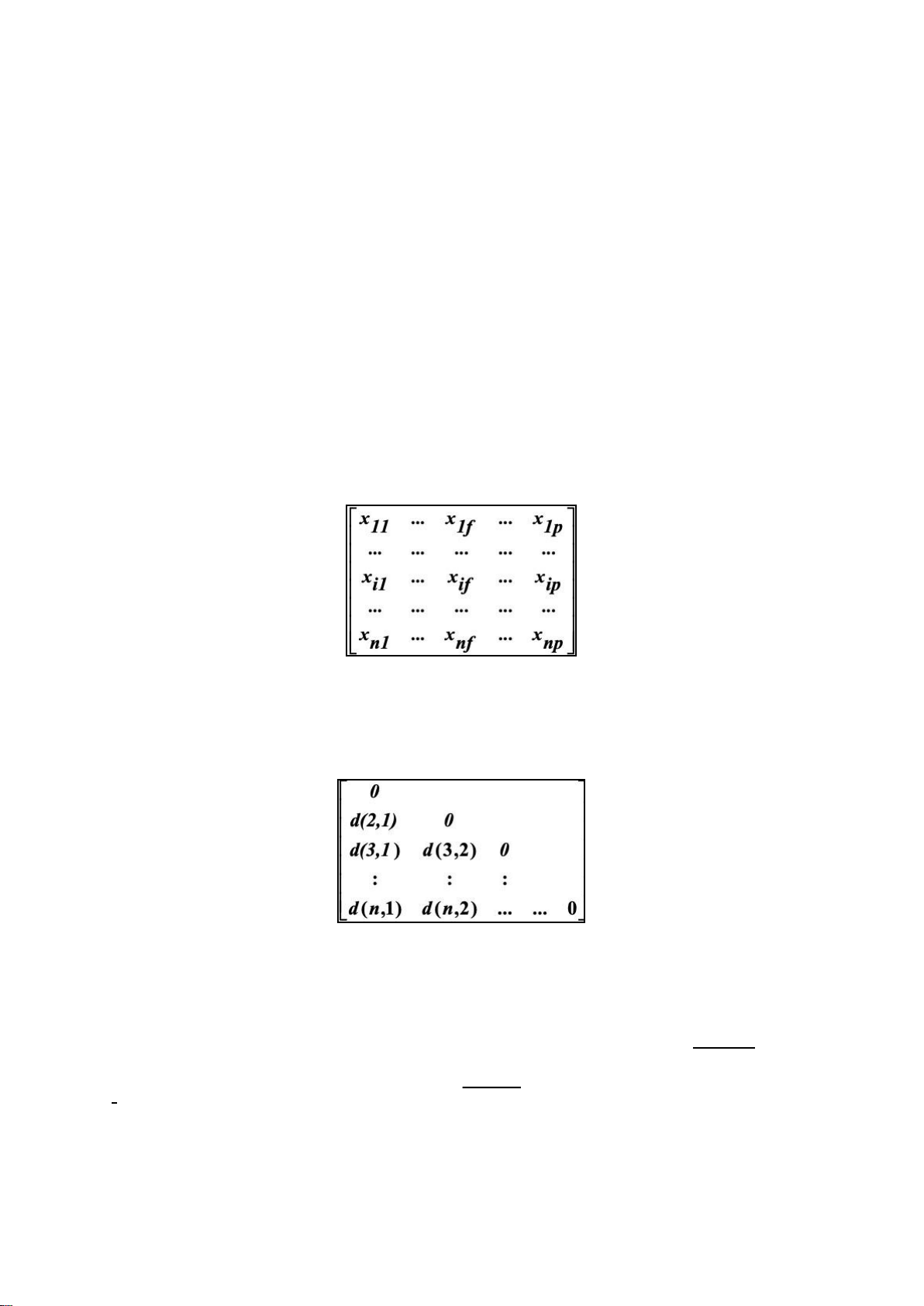
Data Matrix and Dissimilarity Matrix
Data matrix - n data points with p-dimensions have 2 modes Data matrix
Dissimilarity matrix - n data points, but registers only the distance, a triangular matrix. have single mode Dissimilarity matrix
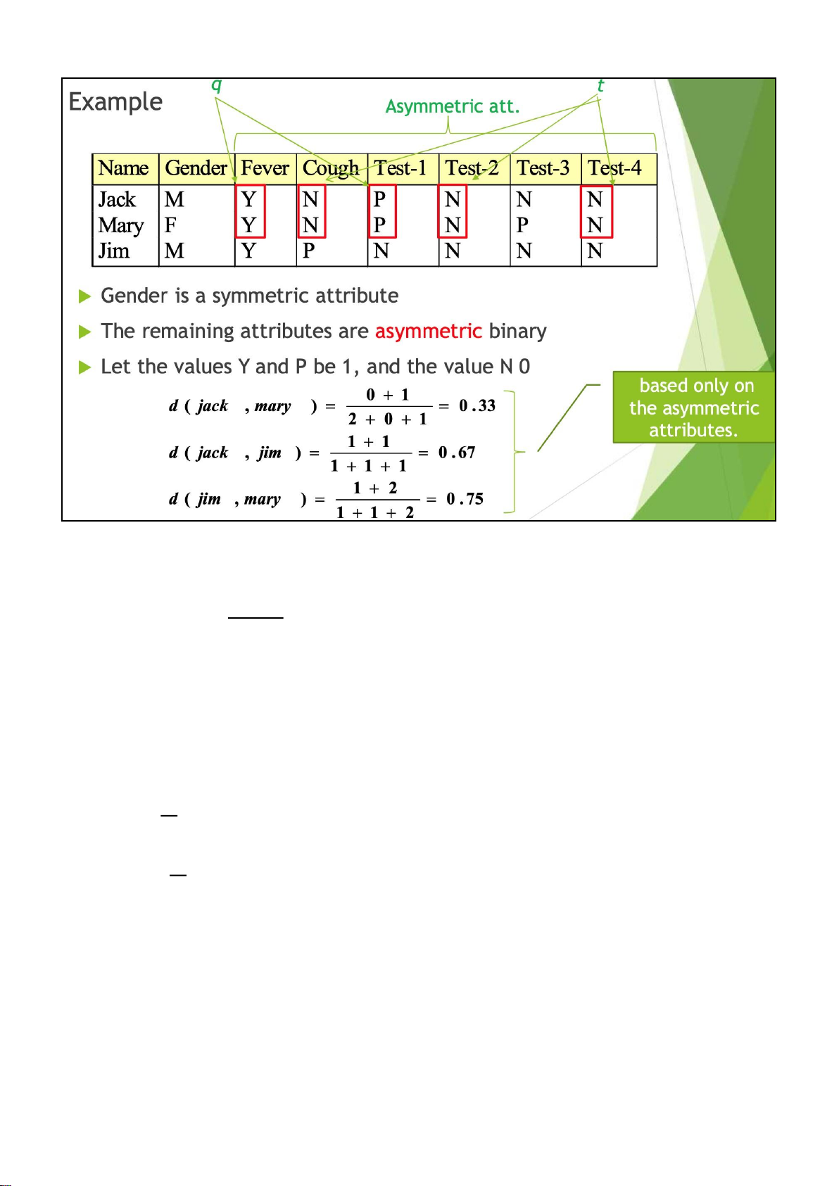
Proximity Measure for Nominal Att.
Def - can take 2 or more state ( example: red ; yellow ; blue ; green ) Method
- Simple matching. d(i, j) = p −p m lOMoAR cPSD| 23136115
Proximity Measure for Binary Att. •
A contingency table for binary data •
Distance measure for symmetric binary variables: d(i, j) = q +rr ++ss + t •
Distance measure for asymmetric binary variables: d(i, j) = q +r +r +s s •
Jaccard coefficient (similarity measure for asymmetric binary variables): q
simjaccard(i, j) = q + r + s •
Note: Jaccard coefficient is the same as “coherence”:
coherence(i, j) = sup(i) + ssuupp((ij,)j−) sup(i, j) = (q + r) +qq + s − q lOMoAR cPSD| 23136115
Standardizing Numeric Data
• Z-score: z = x −σμ
• X: raw score to be standardized, μ: mean of the population, σ: standard deviation
• Alternative way: calculate the mean absolute deviation : 1
sf = n(|x1f − mf | + |x2f − mf | + ... + |xnf − mf |) where mf =
1n(x1f + x2f + ... + xnf) lOMoAR cPSD| 23136115
• Standardized measure (Z-Score): zif = xif −sf mf
• Using mean absolute deviation is more robust than using standard deviation Orbital Variables
An ordinal variable can be discrete or continuous
Order is important, e.g., rank Can be treated
like interval-scaled replace Xif by their rank rif
ϵ(1,...,Mf ) map the range of each variable
onto [0, 1] by replacing i-th object in the f-th variable by
zif = Mriff −−11
compute the dissimilarity using methods for interval- scaled variables Cosine Similarity
• A document can be represented by thousands of attributes, each recording the
frequency of a particular word (such as keywords) or phrase in the document.
• Other vector objects: gene features in micro-arrays, ...
• Applications: information retrieval, biologic taxonomy, gene feature mapping, ... •
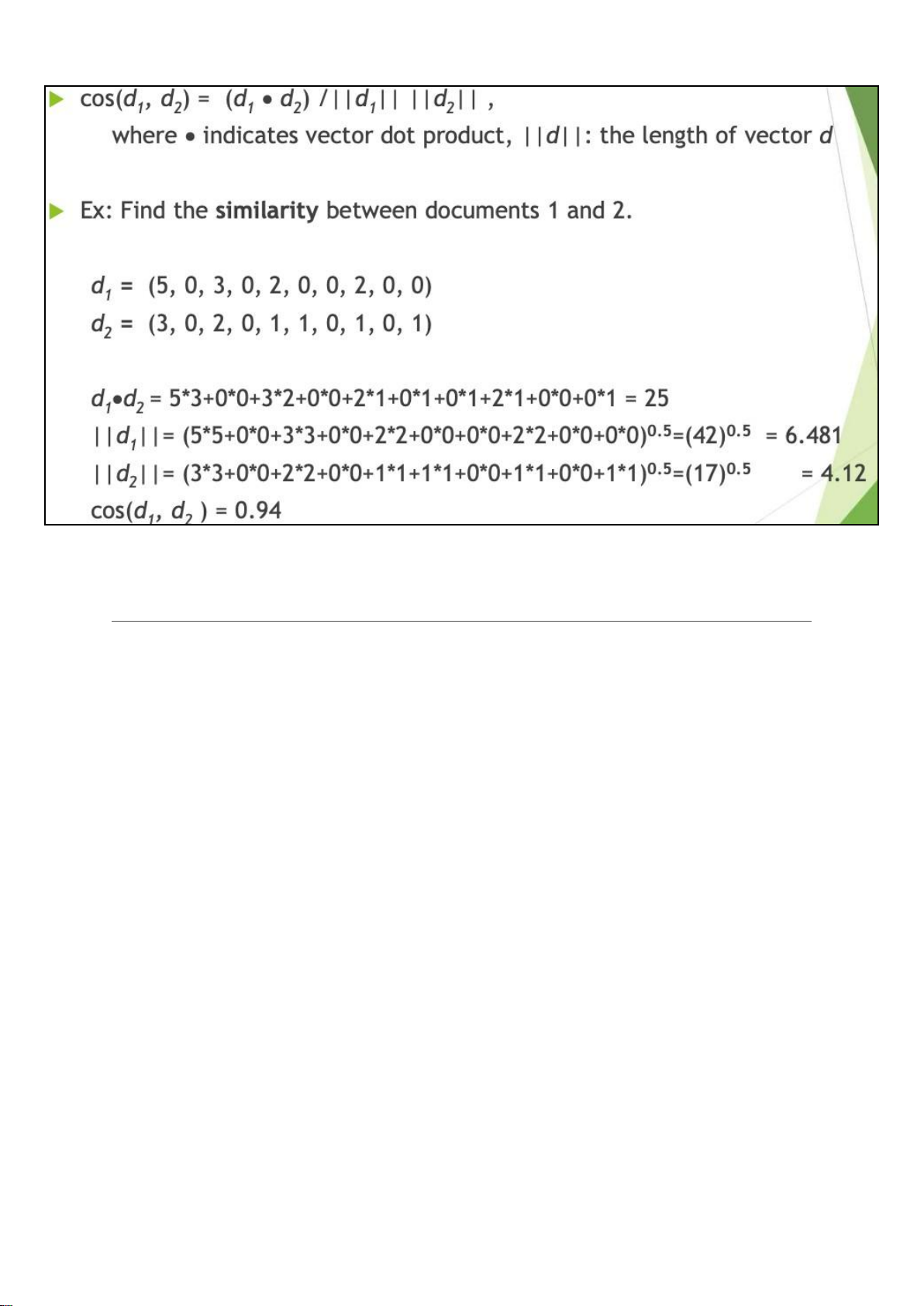
Cosine measure: If d1 and d2 are two vectors (e.g., term-frequency vectors), then:
cos(d1,d2) = (d1 ∙ d2)/||d1||||d2|| where • indicates vector dot product, || d||: the length of vector d lOMoAR cPSD| 23136115
Chapter 3 : Data Preprocessing
Data quality : Why preprocess the data
1. Measures for data quality: A multidimensional view
2. Accuracy: correct or wrong, accurate or not
3. Completeness: not recorded, unavailable, ...
4. Consistency: some modified but some not, dangling, ...
5. Timeliness: timely update?
6. Believability: how trustable the data are correct?
7. Interpretability: how easily the data can be understood?
Major task in Data Preprocessing
1. Data cleaning - Fill in missing values, smooth noisy data, identify or remove
outliers, and resolve inconsistencies
2. Data integration - Integration of multiple databases, data cubes, or files lOMoAR cPSD| 23136115 3. Data reduction • Dimensionality reduction • Numerosity reduction • Data compression
4. Data transformation and data discretization • Normalization
• Concept hierarchy generation Data Cleaning
Data in the Real World Is Dirty: Lots of potentially incorrect data, can fall into these
category : Incomplete ; Noisy ; Inconsistent ; Intentional.
Example: instrument faulty, human or computer error, transmission error
1. Incomplete (Missing) data - lacking attribute values, lacking certain attributes of
interest, or containing only aggregate data. Cause may be due to : 1. Equipment malfunction
2. Inconsistent with other recorded data and thus deleted
3. Data not entered due to misunderstanding
4. Certain data may not be considered important at the time of entry
5. Not register history or changes of the data
Example: Occupation = “ ” (missing data)
2. Noisy Data - containing noise, errors, or outliers. To be more specific is random
error or variance in a measured variable. Cause may be due to :
1. Faulty data collection instruments 2. Data entry problems 3. Data transmission problems 4. Technology limitation
5. Inconsistency in naming convention
• Other Data Problem which require data cleaning : Duplicate records lOMoAR cPSD| 23136115 Incomplete data Inconsistent data
Example: Salary = “−10” (an error)
3. Inconsistent Data - containing discrepancies in codes or names
Example: Age = “42”, Birthday = “03/07/2010” ; Was rating “1, 2, 3”, now rating “A, B,
C” ; discrepancy between duplicate records.
4. Intentional Data - also know as Disguised missing Data Example: Jan. 1
as everyone’s birthday?
How to Handle Missing Data
1. Ignore the tuple: usually done when class label is missing (when doing
classification) not effective when the % of missing values per attribute varies considerably
2. Fill in the missing value manually: tedious + infeasible?
3. Fill in it automatically with
• A global constant : e.g., “unknown”, a new class?! • The attribute mean
• The attribute mean for all samples belonging to the same class: smarter
• The most probable value: inference-based such as Bayesian formula or decision tree
How to Handle Noisy Data 1. Binning
First sort data and partition into (equal-frequency) bins
Then one can smooth by bin means, smooth by bin median, smooth by bin boundaries. 2. Regression
Smooth by fitting the data into regression functions 3. Clustering Detect and remove outliers lOMoAR cPSD| 23136115
4. Combined computer and human inspection
Detect suspicious values and check by human (e.g., deal with possible outliers) Data Cleaning as a Process
Data discrepancy detection
1. Use metadata (e.g., domain, range, dependency, distribution) 2. Check field overloading
3. Check uniqueness rule, consecutive rule and null rule 4. Use commercial tools
Data scrubbing: use simple domain knowledge (e.g., postal code, spellcheck)
to detect errors and make corrections
Data auditing: by analyzing data to discover rules and relationship to
detect violators (e.g., correlation and clustering to find outliers) Data migration and integration
1. Data migration tools: allow transformations to be specified
2. ETL (Extraction/Transformation/Loading) tools: allow users to specify
transformations through a graphical user interface
Integration of the two processes
3. Iterative and interactive (e.g., Potter’s Wheels) Data Integration
Def : Combines data from multiple sources into a coherent store • Schema
integration - Integrate metadata from different sources ( Example:
A .cust − id ≡ B.cust − # )
• Entity identification problem:
• Identify real world entities from multiple data sources, e.g., Bill Clinton = William Clinton
• Detecting and resolving data value conflicts
• For the same real-world entity, attribute values from different sources are different
• Possible reasons: different representations, different scales, e.g., metric vs. British units lOMoAR cPSD| 23136115
Handling Redundancy in Data Integration
• Redundant data occur often when integration of multiple databases
1. Object identification: The same attribute or object may have different names in different databases
2. Derivable data: One attribute may be a “derived” attribute in another table, e.g., annual revenue
• Redundant attributes may be able to be detected by correlation analysis and covariance analysis
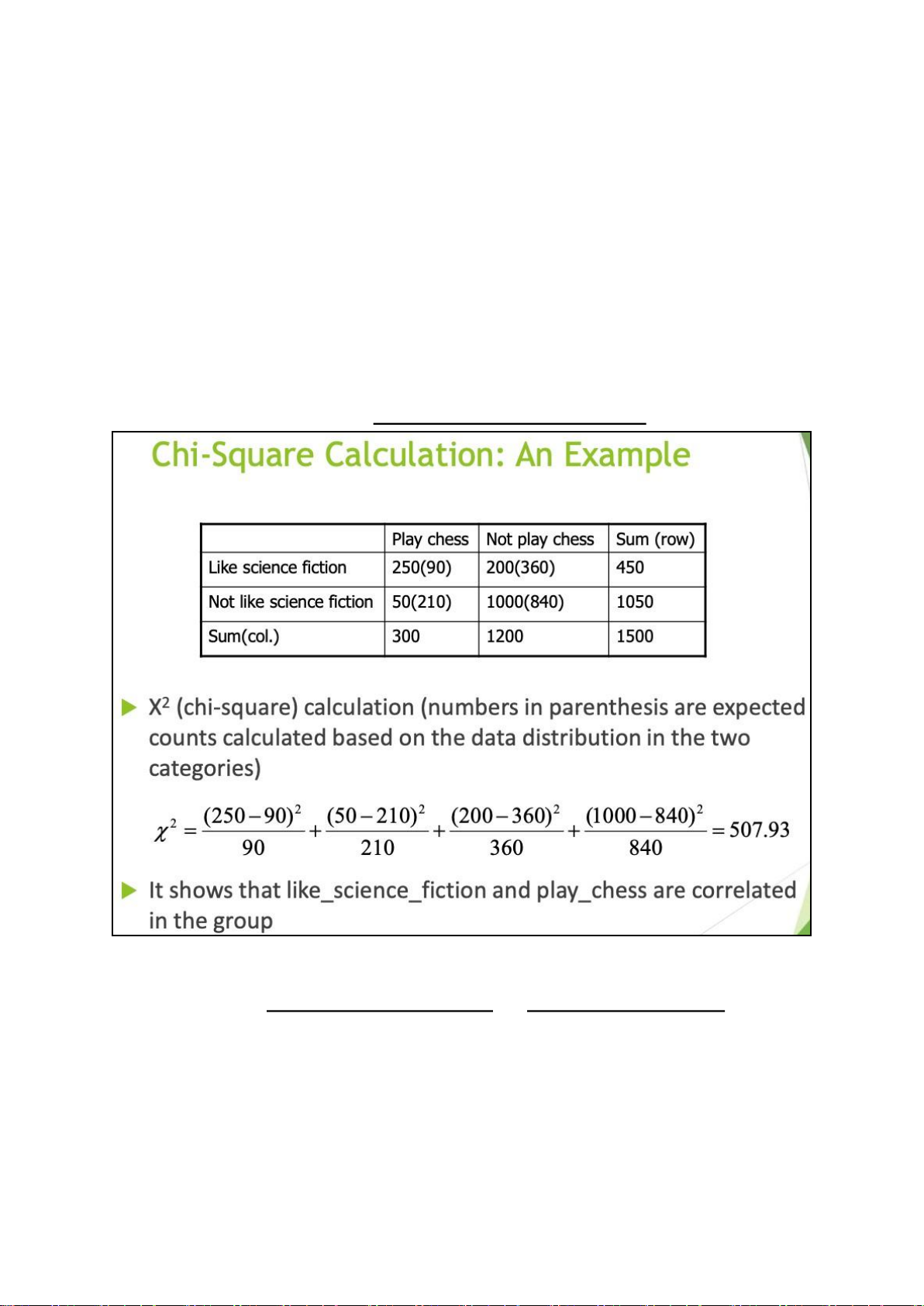
Correlation Analysis (Nominal Data)
X2 = ∑ (ObservEexdp−ecEtexdpected)2
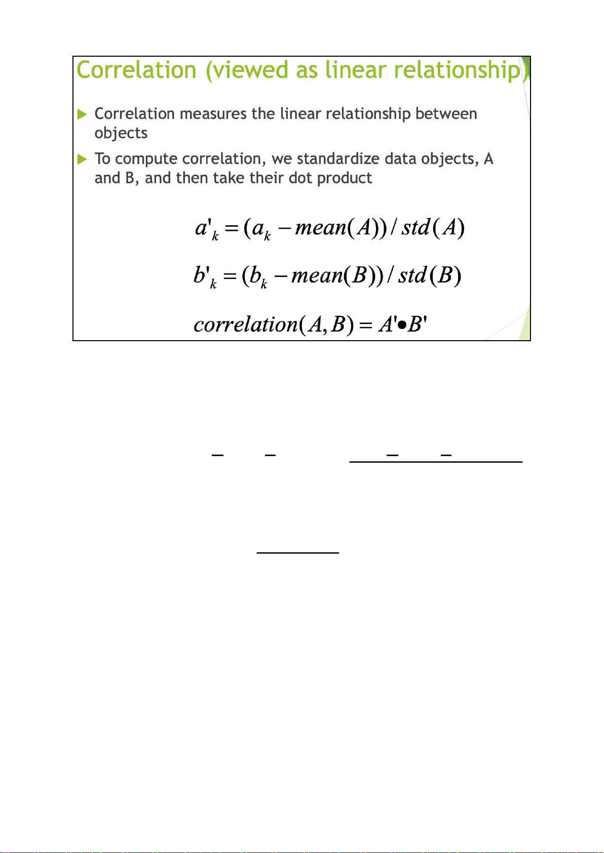
Correlation Analysis (Numeric Data)
rA,B = nσAσB=
i=1 (naiσbAiσ)B− nA¯B¯ ∑ni=1 (ai − A¯)(bi − B¯) ∑n
• If rA,B > 0, A and B are positively correlated (A’s values increase as B’s). The higher, the stronger correlation.
• rA,B = 0: independent;rAB < 0: negatively correlated lOMoAR cPSD| 23136115
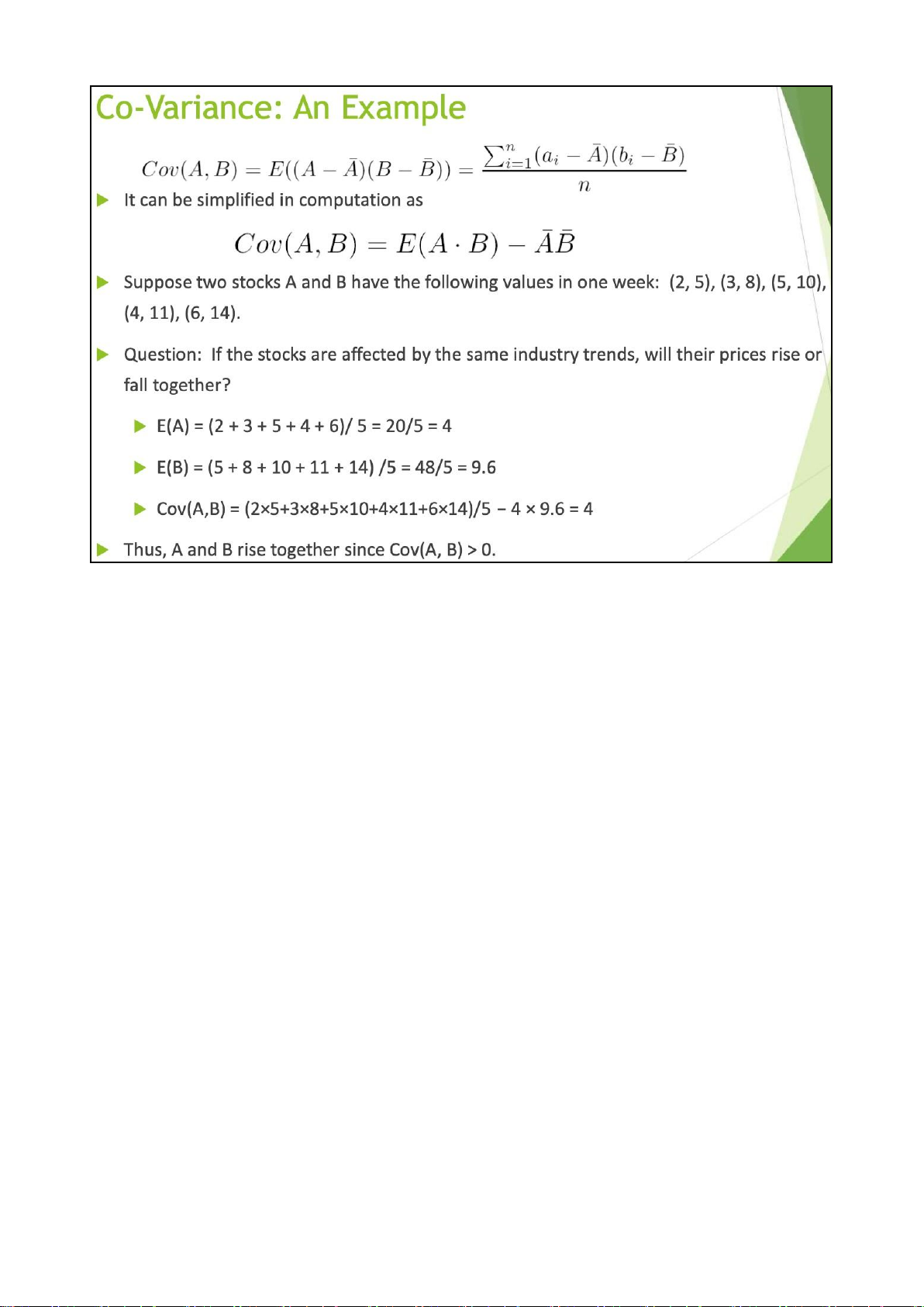
Covariance (Numeric Data)
Covariance is similar to correlation
Cov(A,B) = E[(A − A)(B − B)] = ∑ni=1 (ai −nA)(bi − B)
Correlation Coefficient : rA,B = CoσvA(σAB,B)
• Positive covariance: If CovA,B > 0, then A and B both tend to be larger than their expected values. lOMoAR cPSD| 23136115
• Negative covariance: If CovA,B < 0 then if A is larger than its expected value, B is
likely to be smaller than its expected value.
• Independence: CovA,B = 0 but the converse is not true.
Data Reduction Strategies
Data reduction: Obtain a reduced representation of the data set that is
much smaller in volume but yet produces the same (or almost the same) analytical results
Why data reduction? — A database/data warehouse may store terabytes
of data. Complex data analysis may take a very long time to run on the complete data set. The Strategies:
1. Dimensionality reduction -
1. Curse of Dimensionality - As the dimensionality of data increases,
the data becomes more sparse and the density and distance
between points, which are crucial for clustering and outlier analysis,