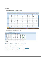
Phân Tích Hồi Quy & Logistic môn Thống kê trong kinh tế và kinh doanh | Trường Đại học Kinh tế Quốc dân

Table of Contents
Task 1: Regression Analysis------------------------------------------------------------------------------------- 2
1. Determine best predictor of Winnings................................................................................................2
2. The First Regression Model Analysis................................................................................................3
3. The Second Regression Model Analysis............................................................................................4
4. Determine the better Estimated Regression Equation.......................................................................5
TASK 2: Logistic regression analysis------------------------------------------------------------------------- 8
a. Determine the better Estimated Regression Equation.......................................................................8
b. Interpretation......................................................................................................................................8
c. MiniTab's Binary Logistic Regression...............................................................................................8
d. Test for overall significance of the model..........................................................................................9
e. Test for significance of independent variables.................................................................................10
f. Estimation Logistic Regression Model..............................................................................................11
g. Estimated Odds Ratio for the orientation program..........................................................................12
h. Reccomendation...............................................................................................................................12
Task 3:------------------------------------------------------------------------------------------------------------- 13
a.Use factor analysis to find the factors...............................................................................................13
b.Run regression model........................................................................................................................18 1 Task 1: Regression Analysis
a. Determine best predictor of Winnings.
Let ŷ is the predicted winnings and x1, x2, x3, x4 are the given number of poles won,
the number of wins, the number of top 5 finishes and number of top 10 finishes.
In order determine which of the four variables provide the best single predictor for
winnings, determine the estimated regression equation as well as the p value for each
single independent variables for the given data, do as follows:
Step 1. Open the web file NASCAR. Click the data tab on the ribbon.
Step 2. In the Analysis group, click Data Analysis.
Step 3. Choose Regression from the list of Analysis Tools.
Step 4. When the Regression dialog box appears enter the following:
Enter G1: G36 in the Input Y Range box.
Enter C1:F36 in the Input X Range box. Select Labels. Select Confidence Level box. Select Output Range.
Enter H3 in the output range box. Click OK.
Then we receive the output below: Regression Statistics Multiple R 0.905808159 R Square 0.820488422 Adjusted R Square 0.796553544 Standard Error 581382.1968 Observations 35 ANOVA 2 df SS MS F Significance F Regression 4 4.63473E+13 1.15868E+13 34.28003482 8.61942E-11 Residual 30 1.01402E+13 3.38005E+11 Total 34 5.64875E+13 Standard Coefficients Error t Stat P-value Lower 95% Upper 95% Intercept
3140367.087 184229.0243 17.04599533 5.59454E-17 2764121.225 3516612.949 Poles
-12938.9208 107205.0751 -0.12069317 0.904738802 -231880.892 206003.0513 Wins
13544.81269 111226.2163 0.12177716 0.90388757 -213609.425 240699.0507 Top 5
71629.39328 50666.86771 1.413732416 0.167734163 -31846.1550 175104.9416 Top 10
117070.5768 33432.88382 3.501659548 0.001470314 48791.51907 185349.6346
The estimated regression equation is as follows:
ŷ = 3140367.09 - 12938.92x1 - 13544.81x2 + 71629.39x3 + 117070.58x4
From the above output, it can be observed that the value corresponding to p � test
each of the individual variables, it has been found that Top ten finishes ( value- 0 ) p
making it the best predictor out of four.
b. The First Regression Model Analysis
The regression equation is obtained from the coefficient of the regression output which is highlighted in yellow
y = 3140367.09 - 12938.92 (Poles) + 13544.81 (Wins) + 71629.39 (Top 5) + 117070.58 (Top 10)
Checking the significance for each variable. For each beta coefficient we test the following hypothesis: Ho: ꞵi =0 H1: ꞵi 0 3
Next we check the value for the variable in the regression output and check if the p value is p
less than 0.05, if it is less than 0.05, then we reject the null hypothesis and conclude that the variable is significant.
We see that the value for Poles, p
Wins, Top 5 is greater than 0.05, hence these variables are not significant predictor of y. The
p value for Top 10 is less than 0.05, hence it is significant predictor of y
c. The Second Regression Model Analysis. The dummy variables Top2-5(x x
1) and Top 6-10( 2) is defined as follows:
x = 1 if the driver finishes between second and fifth place, 0 otherwise 1 Similarly,
x = 1 if the driver finishes between sixth and ten place, 0 otherwise 2
With this definition the, values corresponding to finishes are as follows: Finishes x x 1 2 Top 20 0 0 Top 2-5 1 0 Top 6-10 0 1
Using the dummy variables the multiple regression model turns out to be as follows: y = ꞵ x x 2 + ꞵ1 1 + ꞵ2 2 + ε
Now use the above steps with modifications in, Input Y range (11:136) and Input X range
(B1:H36). The table is as follows: Regression Statistics Multiple R 0.745528722 R Square 0.555813075 Adjusted R Square 0.496588152 Standard Error 914530.8939 4 Observations 35 ANOVA Significance df SS MS F F Regression 4
3.13965E+13 7.85E+12 9.384783 4.82729E-05 Residual 30 2.5091E+13 8.36E+11 Total 34 5.64875E+13 Coefficients Standard Error t Stat P-value Lower 95% Upper 95% Intercept 3716894.478 233988.0995 15.88499 3.78E-16 3239027.029 4194761.928 Poles 396521.5014
143131.9522 2.630594 0.013324 84209.46929 668833.3356 Wins 819078.2833 289239.414 2.831835 0.008188 228372.5969 1409783.97 Top 2-5 -690351.2587 864664.8253 -0.7984 0.430912 -2456232.41 1075529.892
Top 6-10 -1658939 .396 1639745 519 -1.0117 0 31997 -5009944.49 1689869.698
The estimated multiple regression equation is as follows: ŷ = 3716894.478+376521.5014x x x x
1 +819078.283 2 - 690351.259 3 -1658937.396 4
d. Determine the better Estimated Regression Equation. Model 1:
ŷ = 3140367.09 - 12938.92x1 - 13544.81x2 + 71629.39x3 + 117070.58x4 Df Coefficients Standard Error t Stat Pr > |t| Intercept 1 3140367.087 184229.0243 17.04599533 <.0001 Poles 1 -12938.9208 107205.0751 -0.120693174 0.9047 5 Wins 1 13544.81269 111226.2163 0.12177716 0.9039 Top 5 1 71629.39328 50666.86771 1.413732416 0.1677 Top 10 1 117070.5768 33432.88382 3.501659548 0.0015 Model 2: ŷ = 3716894.478+376521.5014x x x x
1 +819078.283 2 - 690351.259 3 -1658937.396 4 Df Coefficients Standard Error t Stat Pr > |t| Intercept 1 3716894.478 233988.0995 15.88499 <.0001 Poles 1 396521.5014 143131.9522 2.630594 0.9047 Wins 1 819078.2833 289239.414 2.831835 0.0325 Top 2-5 1 -690351.2587 864664.8253 -0.7984 <.0001 Top 6-10 1 -1658939 .396 1639745 519 -1.0117 0.0015
For unit increase in Top_2_5 that is for each additional increase in Top 2-5 finishes, there is
around 188700 dollars increase we can expect in winning dollars Wins
For each unit increase in the no. of wins, we can expect around 819078.2833
dollars increase in winning dollars Poles
As per the data, it looks like Poles and winnings are inversely related. i.e for every increase in
the poles there is around 12.9K dollars loss in the winning dollars
So, except poles all other variables are directly proportional to the winning dollars 6
Though the adjusted R-sqr for both the models is the same as 79%, the variables are most
significant and less correlated in model 2.
Hence Model 2 is preferred over Model 1
Interpretation of Regression coefficients for Model 2: Top_6_10
For unit increase in Top_6_10 that is for each additional increase in Top 6-10 finishes, there is
around 1658939 .396 dollars decrease we can expect in winning dollars Top_2_5
For unit increase in Top_2_5 that is for each additional increase in Top 2-5 finishes, there is
around 690351.2587 dollars decrease we can expect in winning dollars Wins
For each unit increase in the no. of wins, we can expect around 819078.2833
dollars increase in winning dollars Conclusion:
Model 2 which is based on the new variables is recommended than the first one.
1. Except poles, all the variables are significant and at a 5% level of significance and so
has an effect on the response variable;
Whereas in the first model except for Top10 all are insignificant
2. The maximum correlation that we can notice in model 2 variables is less than 50%.
But for model 1, all the variables are highly correlated with a max correlation of 90%
Though the adjusted R-sqr for both the models is the same as 79%, the variables are
most significant and less correlated in model 2. 7
Task 2: Logistic regression analysis
a. Determine the better Estimated Regression Equation.
The dependent variable y is defined as follows: Th
e logistic regression equation relating and to is:
Where is the constant term in a regression equation and are the coefficients of the independent variables , , …, b. Interpretation.
We know that = 0 means that the student did not attend the orientation program. Therefore, we have E(y) as follows:
Therefore, when = 0 then E(y) is the estimate of the probability that the student returns to
Lakeland for sophomore year, given that the student did not attend the orientation program,
which means = 0. This is still dependent on the value of or the student's GPA.
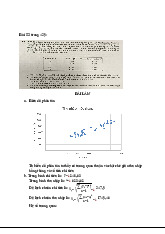
c. MiniTab's Binary Logistic Regression. Deviance Residuals: Min 1Q Median 3Q Max -1.9610 -0.4828 0.2848 0.5980 1.8154 Coefficients: 8 Predictor Coefficient Std. Error z p Constant -6.890 1.750 -3.94 0 GPA 2.539 0.673 3.77 0 Program 1.561 0.563 2.77 0.006
Null deviance: 128.207 on 99 degrees of freedom
Residual deviance: 80.338 on 97 degrees of freedom Log-Likelihood = - 40.169 => Logistic model: The estimated Logit model is:
d. Test for overall significance of the model.
The hypotheses for the test of overall significance are:
One or both of the parameters is not equal to zero.
Null deviance: 128.207 on 99 degrees of freedom
Residual deviance: 80.338 on 97 degrees of freedom
Calculate Chi-squared statistic: has 2 degrees of freedom. Since
Reject => The overall model is significant
Therefore, we can conclude that there is a significant relationship between the independent
variables and dependence variables. 9
e. Test for significance of independent variables.
A z-test can be used to determine whether each of the individual independent variables is
making a significant contribution to the overall model.
+) For the independent variable , the hypotheses are:
If the null hypothesis is true, the value of the estimated coefficient divided by its standard.
error follows a standard normal probability distribution.
Output for coefficients for Lakeland.
The corresponding p-value is 0.000161.
At � = .05, we reject , which mean is significant.
+) For the independent variable , the hypotheses are:
If the null hypothesis is true, the value of the estimated coefficient divided by its standard
error follows a standard normal probability distribution.
The corresponding p-value is 0.006.
At � = .05, we reject , which mean is significant.
Since at � = .05 we can reject both the hypotheses, we can conclude that both the independent
variables are statistically significant. 10
f. Estimation Logistic Regression Model. The estimated Logit model is:
The estimate of the probability that students with a 2.5 grade point average who did not attend
the orientation program will return to Lakeland for their sophomore year is obtained by substituting the values And
So the estimate of the probability that students with a 2.5 grade point average who did not attend
the orientation program will return to Lakeland for their sophomore year is 0.3668, which means 36.68%.
The estimate of the probability that students with a 2.5 grade point average who attended the
orientation program will return to Lakeland for their sophomore year is obtained by substituting the values And
So the estimate of the probability that students with a 2.5 grade point average who attended the
orientation program will return to for their sophomore year is 0.734, which means 73.4%.
g. Estimated Odds Ratio for the orientation program.
The estimated odds ratio measures the estimated impact on the probability when only one
independent variable is increased by one unit. This is given as estimated odds ratio=
The estimated odds ratio for the orientation program, is given by: 11
So, the estimated odds ratio for the orientation program is 4.763. The value 4.763 tells us that the
odds of students who attended the orientation program continuing are 4.763 times greater than
for students who did not attend the program. h. Reccomendation.
We can observe from part (e) that students who have participated in the orientation program have
substantially better chances of continuing.
As can be seen from section (f), the probability estimate for students with a 2.5-grade point
average is 0.37 percent of those who did not participate in the orientation session will return for their sophomore year.
And the estimated likelihood that students who participated in the orientation program and had a
2.5-grade point average would return for their sophomore year is 0.73.
The probabilities of students who participated in the orientation program returning as
sophomores are 1.76 times higher than the projected odds, as can also be shown in portion (g) above.
From the results obtained in part (f) and part (g), we can conclude that the orientation program is
of great value in making the students return for the sophomore year.
We have established that there is a significant relationship between the attendance to the
orientation program and the student's return to Lakeland for sophomore year. This means that the
attendance to the program significantly affects whether a student would return to Lakeland.
Additionally, the estimated odds ratio for the orientation program is 4.762. This means that
attendance to the program significantly affects the probability of a student returning to Lakeland
by 4.762 times, that is, if they attend the orientation program, they are more likely to return to
Lakeland. Hence, it would be a good recommendation to make the orientation a required activity
because it has a positive correlation with the student's return.
So, it is recommended that the orientation program must be a required activity. Task 3: Factor Analysis
a.Use factor analysis to find the factors
Table file “FA Table” attached is a questionnaire with data given in excel file “FA1”.
Use this data, first use factor analysis to find the factors. 12 FACTOR
/VARIABLES CSHT1 CSHT2 CSHT3 CSHT4 CSHT5 CSHT6 CSDT1 CSDT2 CSDT3
CSDT4 CSDT5 MTS1 MTS2 MTS3 MTS4 MTS5 MTS6 MTS7 LTDT1 LTDT2 LTDT3 LTDT4
NNL1 NNL2 NNL3 NNL4 NNL5 NNL6 CPCT1 CPCT2 CPCT3 CPCT4 SAT1 SAT2 SAT3 SAT4 SAT5 /MISSING LISTWISE
/ANALYSIS CSHT1 CSHT2 CSHT3 CSHT4 CSHT5 CSHT6 CSDT1 CSDT2 CSDT3 CSDT4
CSDT5 MTS1 MTS2 MTS3 MTS4 MTS5 MTS6 MTS7 LTDT1 LTDT2 LTDT3 LTDT4 NNL1
NNL2 NNL3 NNL4 NNL5 NNL6 CPCT1 CPCT2 CPCT3 CPCT4 SAT1 SAT2 SAT3 SAT4 SAT5 /PRINT INITIAL EXTRACTION
/CRITERIA MINEIGEN(1) ITERATE(25) /EXTRACTION PC /ROTATION NOROTATE /METHOD=CORRELATION. Factor Analysis Communalities Initial Extraction CSHT1 1,000 0,766 CSHT2 1,000 0,862 CSHT3 1,000 0,656 CSHT4 1,000 0,657 CSHT5 1,000 0,835 CSHT6 1,000 0,748 CSDT1 1,000 0,713 CSDT2 1,000 0,625 CSDT3 1,000 0,655 CSDT4 1,000 0,611 CSDT5 1,000 0,735 13 MTS1 1,000 0,487 MTS2 1,000 0,766 MTS3 1,000 0,776 MTS4 1,000 0,763 MTS5 1,000 0,802 MTS6 1,000 0,566 MTS7 1,000 0,654 LTDT1 1,000 0,840 LTDT2 1,000 0,791 LTDT3 1,000 0,678 LTDT4 1,000 0,781 NNL1 1,000 0,860 NNL2 1,000 0,661 NNL3 1,000 0,776 NNL4 1,000 0,519 NNL5 1,000 0,687 NNL6 1,000 0,664 CPCT1 1,000 0,919 CPCT2 1,000 0,778 CPCT3 1,000 0,827 CPCT4 1,000 0,714 SAT1 1,000 0,837 SAT2 1,000 0,831 SAT3 1,000 0,646 SAT4 1,000 0,625 SAT5 1,000 0,786
Extraction Method: Principal Component Analysis. Total Variance Explained Component Initial Eigenvalues Extraction Sums of Squared Loadings 14 Total % of
Variance Cumulative % Total % of Variance Cumulative % 1 8,362 22,600 22,600 8,362 22,600 22,600 2 4,682 12,654 35,254 4,682 12,654 35,254 3 3,162 8,545 43,799 3,162 8,545 43,799 4 2,392 6,466 50,265 2,392 6,466 50,265 5 1,996 5,394 55,659 1,996 5,394 55,659 6 1,942 5,248 60,908 1,942 5,248 60,908 7 1,714 4,633 65,541 1,714 4,633 65,541 8 1,371 3,704 69,246 1,371 3,704 69,246 9 1,273 3,441 72,686 1,273 3,441 72,686 10 0,883 2,386 75,072 11 0,859 2,322 77,394 12 0,784 2,120 79,513 13 0,719 1,944 81,458 14 0,617 1,668 83,126 15 0,605 1,634 84,760 16 0,536 1,448 86,208 17 0,478 1,291 87,499 18 0,441 1,193 88,692 19 0,421 1,137 89,829 20 0,398 1,076 90,905 21 0,370 1,001 91,906 22 0,363 0,980 92,886 23 0,314 0,847 93,734 24 0,293 0,793 94,526 25 0,276 0,747 95,273 26 0,249 0,672 95,946 27 0,246 0,666 96,611 28 0,205 0,553 97,165 29 0,186 0,501 97,666 30 0,160 0,433 98,099 15 31 0,148 0,400 98,499 32 0,143 0,385 98,884 33 0,116 0,314 99,198 34 0,096 0,258 99,457 35 0,076 0,205 99,662 36 0,064 0,174 99,835 37 0,061 0,165 100,000
Extraction Method: Principal Component Analysis. Component Matrixa Component 1 2 3 4 5 6 7 8 9 CSHT1 0,507
-,458 0,135 0,089 -,360 -,229 -,212 0,060 0,203 CSHT2 0,632 -,489 0,308 0,078 -,265 -,181 -,075 0,115 0,029 CSHT3 0,431
-,279 -,053 0,227 -,348 -,342 0,051 0,000 0,313 CSHT4 0,325
0,614 -,247 0,134 -,106 0,034 0,068 0,260 0,104 CSHT5 0,417
0,638 -,296 0,255 -,002 0,146 -,020 0,259 0,111 CSHT6 0,560
-,435 0,351 0,015 -,220 -,227 -,094 0,067 0,092 CSDT1 0,527
0,051 0,227 -,041 -,067 0,247 0,086 -,457 0,314 CSDT2 0,486
0,201 0,215 -,047 0,167 0,032 0,274 -,343 0,278 CSDT3 0,197
0,622 0,074 0,077 0,144 0,027 0,180 0,178 0,363 CSDT4 -,103
0,318 0,551 -,174 -,007 0,249 0,270 -,172 0,009 CSDT5 0,598 0,463 -,303 ,086 -,007 -,154 -,194 0,049 -,024 MTS1 0,503 -,103 -,003 0,146 -,319 -,114 -,158 -,175 0,178 MTS2 0,345
-,420 0,352 -,343 0,155 0,076 -,158 0,328 0,258 MTS3 0,235 0,115 0,621 -,357 0,060 -,146 0,038 0,340 -,227 MTS4 0,626
0,315 0,276 -,051 -,086 -,177 ,210 -,095 -,319 MTS5 0,650 0,056 0,264 -,322 0,122 -,172 0,087 0,246 -,302 MTS6 0,271 0,123 0,560 -,275 0,003 -,055 0,196 0,159 0,145 MTS7 0,421
0,464 -,052 0,270 -,083 0,079 0,060 0,342 0,230 LTDT1 0,394
-,363 0,055 0,383 0,583 -,220 0,031 -,071 -,094 LTDT2 0,305 -,431 -,030 0,484 0,455 -,257 -,057 ,009 -,026 16 LTDT3 0,369
-,280 0,088 0,136 0,593 -,226 0,150 -,101 0,027 LTDT4 0,630 ,444 0,011 -,184 -,230 -,071 0,216 -,199 -,093 NNL1 0,361
-,568 -,052 0,126 -,246 0,458 0,283 -,034 -,192 NNL2 0,330
-,452 -,042 0,062 -,188 0,432 0,264 0,068 -,216 NNL3 0,421
-,483 -,160 0,227 -,178 0,378 0,312 0,129 0,008 NNL4 0,201
-,107 -,060 0,397 0,091 0,310 0,182 0,381 -,150 NNL5 0,315 0,353 -,165 ,351 -,160 -,396 0,253 -,160 -,202 NNL6 0,501
0,217 -,250 -,012 -,239 -,351 0,109 -,006 -,333 CPCT1 0,537
-,282 -,568 -,441 0,106 0,007 0,133 -,041 ,055 CPCT2 0,557 -,233 -,483 -,409 0,054 ,030 0,080 -,034 0,036 CPCT3 0,506 ,034 -,418 -,539 ,271 -,062 0,106 0,090 0,092 CPCT4 0,480
-,251 -,540 -,328 0,121 0,021 0,029 -,043 0,062 SAT1 0,577
0,083 0,064 -,042 0,045 0,317 -,619 0,040 -,069 SAT2 0,659 0,140 -,022 0,034 -,043 0,150 -,527 -,160 -,215 SAT3 0,654
0,161 0,004 0,214 0,272 0,247 -,081 0,014 0,070 SAT4 0,538
0,117 0,336 0,281 0,214 0,209 0,128 -,154 -,023 SAT5 0,596
0,319 0,172 -0,056 0,088 0,300 -0,356 -0,214 -0,162
Extraction Method: Principal Component Analysis. a. 9 components extracted. b.Run regression model
Use these factor to run regression model to investigate which factors have impact on the satisfaction of investors. REGRESSION /MISSING LISTWISE
/STATISTICS COEFF OUTS R ANOVA /CRITERIA=PIN(.05) POUT(.10) /NOORIGIN /DEPENDENT MSO 17
/METHOD=ENTER CSHT1 CSHT2 CSHT3 CSHT4 CSHT5 CSHT6 CSDT1 CSDT2 CSDT3
CSDT4 CSDT5 MTS1 MTS2 MTS3 MTS4 MTS5 MTS6 MTS7 LTDT1 LTDT2 LTDT3 LTDT4
NNL1 NNL2 NNL3 NNL4 NNL5 NNL6 CPCT1 CPCT2 CPCT3 CPCT4 SAT1 SAT2 SAT3 SAT4 SAT5. Regression Variables Entered/Removeda Model Variables Entered Variables Removed Method 1 SAT5, NNL3, MTS6, NNL5, LTDT3, CPCT3, NNL4, CSHT3, CSHT4, CSDT4, MTS3, CSDT2, NNL6, MTS1, NNL2, CSDT3, LTDT2, MTS7, CSHT6, . Enter CSDT1, SAT4, CPCT4, MTS2, SAT1, SAT3, CSHT1, CPCT2, MTS4, CSDT5, LTDT1, MTS5, SAT2, NNL1, LTDT4, CSHT5, CSHT2, CPCT1b a. Dependent Variable: MSO
b. All requested variables entered. Model Summary Adjusted R Std. Error of Model R R Square Square the Estimate 1 0,645a0,416 0,301 54,6551 18
a. Predictors: (Constant), SAT5, NNL3, MTS6, NNL5, LTDT3, CPCT3, NNL4, CSHT3, CSHT4,
CSDT4, MTS3, CSDT2, NNL6, MTS1, NNL2, CSDT3, LTDT2, MTS7, CSHT6, CSDT1,
SAT4, CPCT4, MTS2, SAT1, SAT3, CSHT1, CPCT2, MTS4, CSDT5, LTDT1, MTS5, SAT2,
NNL1, LTDT4, CSHT5, CSHT2, CPCT1 ANOVAa Sum of Mean Model Squares df Square F Sig. Regression 400323,0 03 37 10819,54 13,622 ,000b Residual 561589,4 97 188 2987,178 Total 961912,500 225 a. Dependent Variable: MSO
b. Predictors: (Constant), SAT5, NNL3, MTS6, NNL5, LTDT3, CPCT3, NNL4, CSHT3, CSHT4,
CSDT4, MTS3, CSDT2, NNL6, MTS1, NNL2, CSDT3, LTDT2, MTS7, CSHT6, CSDT1,
SAT4, CPCT4, MTS2, SAT1, SAT3, CSHT1, CPCT2, MTS4, CSDT5, LTDT1, MTS5, SAT2,
NNL1, LTDT4, CSHT5, CSHT2, CPCT Coefficientsa Standardi zed Unstandardized Coefficie Coefficients nts Model B Std. Error Beta t Sig. 1 (Constant) 61,394 62,449 ,983 ,327 CSHT1 34,813 13,001 ,287 2,678 ,008 CSHT2 -26,525 14,014 -,308 -1,893 ,060 CSHT3 -5,638 8,681 -,053 -,650 ,517 CSHT4 8,793 8,097 ,098 1,086 ,279 CSHT5 -21,114 11,191 -,261 -1,887 ,061 19 CSHT6 11,142 10,102 ,125 1,103 ,271 CSDT1 18,419 10,220 ,157 1,802 ,073 CSDT2 -1,033 8,683 -,009 -,119 ,905 CSDT3 7,418 7,253 ,098 1,023 ,308 CSDT4 -4,731 4,982 -,085 -,950 ,344 CSDT5 30,176 10,155 ,338 2,971 ,003 MTS1 11,946 7,851 ,114 1,522 ,130 MTS2 -10,850 9,119 -,111 -1,190 ,236 MTS3 -16,607 7,668 -,235 -2,166 ,032 MTS4 -1,921 7,260 -,028 -,265 ,792 MTS5 23,886 11,002 ,275 2,171 ,031 MTS6 14,392 8,125 ,176 1,771 ,078 MTS7 2,736 6,673 ,035 ,410 ,682 LTDT1 13,942 10,594 ,148 1,316 ,190 LTDT2 6,390 8,440 ,077 ,757 ,450 LTDT3 23,372 10,496 ,197 2,227 ,027 LTDT4 4,037 11,241 ,047 ,359 ,720 NNL1 15,504 9,274 ,212 1,672 ,096 NNL2 -10,195 8,869 -,095 -1,150 ,252 NNL3 -22,947 8,540 -,282 -2,687 ,008 NNL4 -9,233 3,897 -,161 -2,369 ,019 NNL5 -15,209 8,410 -,169 -1,808 ,072 NNL6 -18,491 7,540 -,234 -2,452 ,015 CPCT1 13,313 12,988 ,186 1,025 ,307 CPCT2 9,686 9,638 ,113 1,005 ,316 CPCT3 -11,338 8,197 -,173 -1,383 ,168 CPCT4 -10,631 9,913 -,112 -1,073 ,285 SAT1 -4,267 13,368 -,043 -,319 ,750 SAT2 -4,303 11,743 -,047 -,366 ,714 20