lOMoAR cPSD| 46988474 NBER WORKING PAPER SERIES
COMPARING PAST AND PRESENT INFLATION Marijn A. Bolhuis Judd N. L. Cramer Lawrence H. Summers Working Paper 30116
http://www.nber.org/papers/w30116
NATIONAL BUREAU OF ECONOMIC RESEARCH 1050 Massachusetts Avenue Cambridge, MA 02138 June 2022
The views expressed herein are those of the authors and do not necessarily reflect the views of the
National Bureau of Economic Research, IMF, its Executive Board, or IMF management.
NBER working papers are circulated for discussion and comment purposes. They have not been
peerreviewed or been subject to the review by the NBER Board of Directors that accompanies official NBER publications. lOMoAR cPSD| 46988474
© 2022 by Marijn A. Bolhuis, Judd N. L. Cramer, and Lawrence H. Summers. All rights reserved.
Short sections of text, not to exceed two paragraphs, may be quoted without explicit permission
provided that full credit, including © notice, is given to the source.
Comparing Past and Present Inflation
Marijn A. Bolhuis, Judd N. L. Cramer, and Lawrence H. Summers NBER Working Paper No. 30116 June 2022 JEL No. C43,E21,E31,E37 ABSTRACT
There have been important methodological changes in the Consumer Price Index (CPI) over time.
These distort comparisons of inflation from different periods, which have become more prevalent
as inflation has risen to 40-year highs. To better contextualize the current run-up in inflation, this
paper constructs new historical series for CPI headline and core inflation that are more consistent
with current practices and expenditure shares for the post-war period. Using these series, we find
that current inflation levels are much closer to past inflation peaks than the official series would
suggest. In particular, the rate of core CPI disinflation caused by Volcker-era policies is significantly
lower when measured using today’s treatment of housing: only 5 percentage points of decline
instead of 11 percentage points in the official CPI statistics. To return to 2 percent core CPI inflation
today will thus require nearly the same amount of disinflation as achieved under Chairman Volcker. Marijn A. Bolhuis Lawrence H. Summers International Monetary Fund
Harvard Kennedy School of Government mbolhuis@imf.org 79 JFK Street Cambridge, MA 02138
Judd N. L. Cramer judd.cramer@gmail.com and NBER lhs@harvard.edu
Full series of headline and core inflation with OER correction and constant weights for different years is
available at: http://larrysummers.com/category/inflation/
1. Introduction
As concerns about US inflation have grown, the Consumer Price Index (CPI) has come under closer
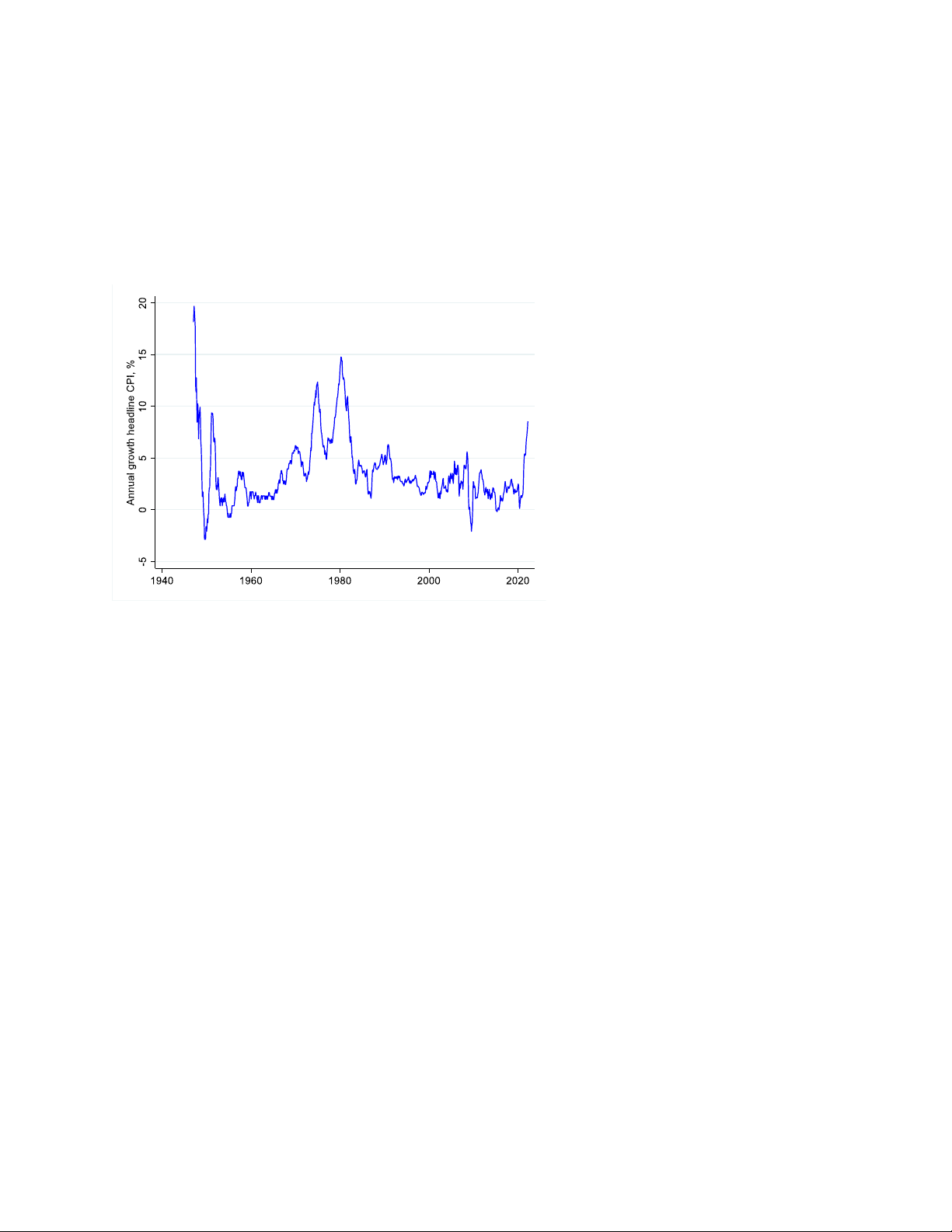
scrutiny.1 The CPI grew 8.3 percent in the twelve months ending in April, down slightly from the
previous month but still well above any other period since 1981 (Figure 1). While a worrying figure,
this remains far below the official March 1980 peak of 14.8 percent. That the headline number had
already fallen to 2.5 percent by July 1983, following the policy decisions of Federal Reserve Board
1 Throughout this paper we use CPI as a shorthand for CPI-U, the Consumer Price Index for All Urban Consumers. lOMoAR cPSD| 46988474
Chairman Paul Volcker, has served as the exemplum of the power of hawkish monetary policy
(Goodfriend and King 2005). Since much less of a decline is needed to return to trend today, some
commenters have suggested that policymakers might be able to decrease inflation towards desired
levels without large macroeconomic consequences (DeLong 2022; Krugman 2022). Yet,
methodological changes in the CPI over time make drawing conclusions from these types of
intertemporal comparisons fraught.
This paper shows that using the movement of the published CPI during past disinflationary
periods to explore the current situation can lead researchers astray. For example, in arguing
against policymakers falling showed that today9s gap between core inflation4which removes volatile food and energy prices4
and real interest rates is approaching about 70 percent of the 1975 gap. We argue against using
official CPI inflation to assess this gap. Most importantly, prior to 1983 measurement of shelter
inflation was mechanically responsive to Federal Reserve interest rate policy via mortgage rates.
This method made pre-1983 peak CPI inflation measures, especially lOMoAR cPSD| 46988474
during the Volcker-era, artificially high at the beginning of the tightening cycle, and declines look artificially fast.
Figure 1: Headline CPI inflation, 1946-present
Source: Bureau of Labor Statistics.
Note: Percent change from 12 months earlier.
To better contextualize the current run-up in inflation, this paper constructs new historical series
for CPI headline and core inflation that are more consistent with current practices and
expenditure shares for the entirety of the post-war period. Using publicly available Bureau of
Labor Statistics (BLS) data for the post-war period, we develop new estimates of CPI headline
and core inflation that can be better compared across time. The full series is available on our
website at http://larrysummers.com/category/inflation/. Our analysis reveals that current
inflation, especially core inflation, is considerably closer to previous peaks than in the official
series. Official core CPI inflation peaked at 13.6 percent in June 1980, whereas we estimate that lOMoAR cPSD| 46988474
core inflation was 9.1 percent in that same month when adjusting for the treatment of shelter
inflation. Our estimates also suggest that the local trough of core CPI inflation in 1983 was
considerably higher than originally reported. Overall, these estimates imply that the rate of core
CPI disinflation caused by Volcker-era policies is significantly lower when measured using the
current treatment of housing: only 5 percentage points of decline instead of 11 percentage
points in the official CPI statistics. To return to 2 percent core CPI today, we thus need
disinflation of a similar magnitude as Chairman Volcker achieved.
Similar issues affect conclusions drawn from comparisons of current inflation with other periods
of elevated inflation. Recent work suggests that the years following World War II have strong
similarities to the current inflation environment (e.g., Rouse et al., 2021; DeLong, 2022). We
show that due to the greater weight of transitory goods components 4especially food and
apparel4 in the index of the 1940s and 1950s, past inflation spikes were higher and more
shortlived than today9s. When using current weights, we estimate that the peak of core CPI
inflation in June 1951 falls from 7.2 to 5 percent, and the peak of headline CPI inflation falls
from 9.4 to just 3.3 percent. These two points serve as a caution against overly optimistic
forecasts of an inexpensive disinflation in the current cycle 4the disinflation that needs to be
achieved now is large by historical standards.
The rest of this paper is structured as follows. Section 2 reviews the methodology used by the
Bureau of Labor Statistics (BLS) informing homeownership costs before and after the changes
introduced in 1983 and suggests that it is natural to expect that past inflation would be lower
using current methods. Section 3 describes the data we employ and different statistical models
we use for creating more consistent CPI measures both to deal with the measurement of 4 lOMoAR cPSD| 46988474
housing and the relatively more estimates for the post-war inflations and disinflations using our measures and shows the current
situation is of a similar magnitude with past episodes. Section 5 offers some concluding observations. lOMoAR cPSD| 46988474
2. Measuring Housing Inflation
Housing is both an investment and a consumption good. On the one hand, it is the largest fixed
investment that most Americans make in their lives.2 On the other hand, it provides a service,
shelter, that is consumed daily. Between 1953 and 1983, the Bureau of Labor Statistics (BLS)
valued homeownership costs for the CPI without disentangling these two qualities. It produced
a measure that broadly captured changes in the expenses of homeowners, taking house prices,
mortgage interest rates, property taxes and insurance, and maintenance costs as inputs. More
specifically, the home-purchase expenditure weight was the net purchase of owner-occupied
houses in the survey period, and the mortgage-interest expenditure weight was the total
interest (undiscounted) that would be paid over half the term on all mortgages incurred during
the survey period (Duggan et al. 1997). Shelter costs were thus directly affected by monetary
policy, due to the effect of the federal funds rate on mortgage rates. This methodology was
without conceptual foundation and its use resulted in a substantial upward bias in the CPI (Gillingham 1980;
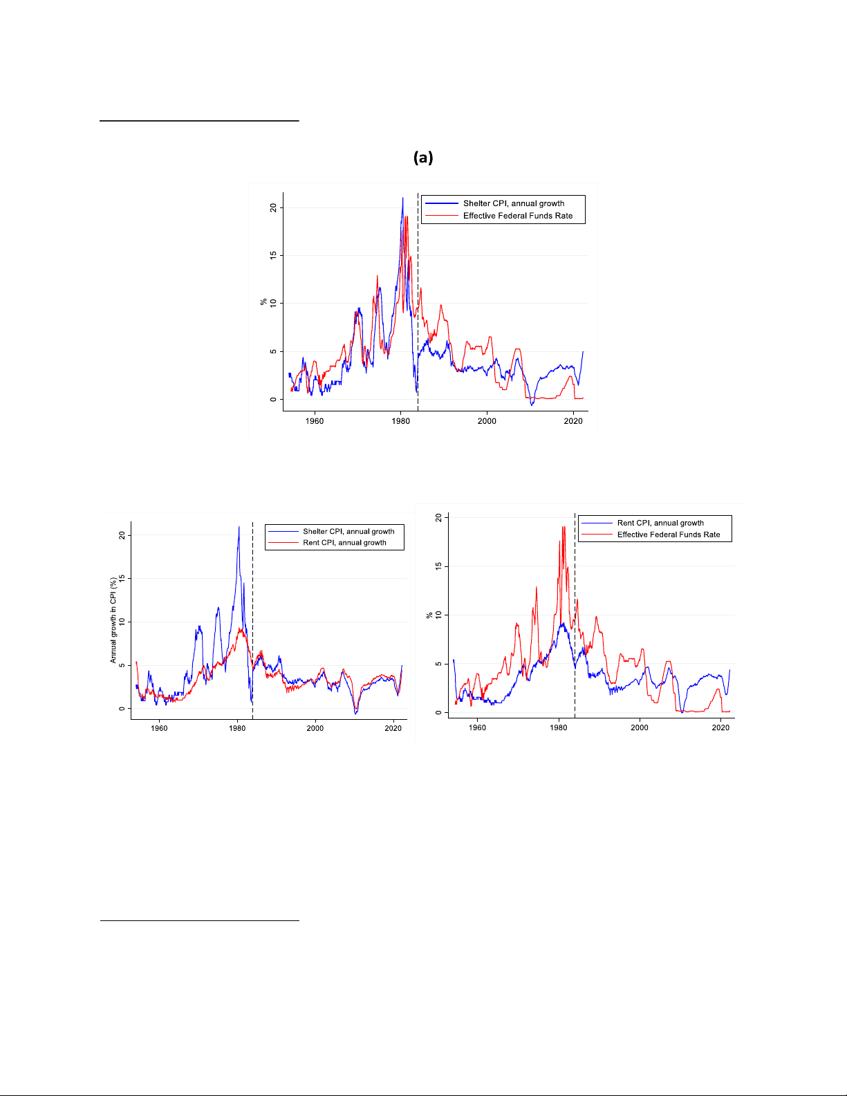
Gillingham 1983). The approach produced a volatile shelter series pre-1983, as shown in Figure
2(a), that moved almost in step with the federal funds rate until 1983. Much more so than rents,
these estimates were responsive to changes in interest rates as seen in the pre-1983 period of
Figure 2(c). During the tightening cycles of 1967-1969, 1972-1974, and 1977-1981, shelter
inflation increased sharply, only to fall precipitously when the pace of tightening slowed down.3
2 This has been the case throughout American history. See, for example, Shelton (1966).
3 Besides the mechanical relationship between monetary policy and homeownership costs, the old approach
faced several other criticisms. Other forms of interest payments, such as credit card spending, were not part 6 lOMoAR cPSD| 46988474
Figure 2: Shelter CPI inflation and the Federal Funds Rate, 1954-present (b) (c)
Source: Bureau of Labor Statistics.
Notes: Percent change from 12 months earlier. Change in OER initiated January 1983.
of the consumer basket. Moreover, consumers either paid for the home purchase price or the mortgage
payments, but not both. Including both led to a larger share of housing in the consumption basket.
Furthermore, the old methodology assumed all homeowners had the same 30-year fixed-rate mortgage. lOMoAR cPSD| 46988474
In 1983, after ten years of study, the BLS exchanged homeownership costs for owners9
equivalent rent (OER) (Gillingham and Lane 1982). By estimating what a homeowner would
receive for their home on the rental market, the BLS stripped away the investment aspect of
housing to isolate owner-occupiers9 consumption of residential services. Since this 1983 shift,
shelter CPI has been much less volatile and much more correlated with rent CPI (Figure 2(b)). Of
course, this shadow price of owner-occupied shelter is not observed. The BLS uses statistical
techniques to infer OER using rental prices for similar units in the area.4 In particular, the
estimated average OER value is determined by a linear regression of imputed rents on property
value, income, and number of rooms from the Consumer Expenditure Survey.5 This procedure is
done for all units, not just newly signed leases or newly purchased houses, with housing units in
the sample queried every six months. Estimated OER will therefore lag spot prices and is
mechanically correlated with rents.6
The 1983 housing changes had large effects on both headline and core measures of inflation. In
December 1982, For the core CPI, it was a full 36.1 percent. In its last month, homeownership costs were reported
4 For a recent discussion of methods see Gindelsky et al. (2019).
5 For complete details, see Chapter 17 of the BLS handbook of methods. The linear regression coefficients are
then applied to decennial census values for the same independent variables to estimate the average owners9
equivalent rent for each segment via the nonlinear regression
㕂㔸㕅 = 㗽Ā + (㗽1 × āÿĀā㕣㕎ý) + (㗽2 × āÿĀā㕣㕎ý2 )+ (㗽3 × 㕖ÿ㕐Āþ㕒)+ (㗽4 × ÿĀĀþĀ) ,
where OER is the predicted value that the home would rent for, propval is the market value of the home,
income is the income of the consumer unit, and rooms is the number of rooms in the house. The BLS repeats
this procedure across different geographic areas. After the modelling process, CPI weights are then
determined by surveys of homeowners.
6 For further discussion of this lag structure, see Bolhuis et al. (2022) 8 lOMoAR cPSD| 46988474
to have declined by 1.7 percent from November to December as the financing, taxes, and
insurance component, which mostly varied with mortgage rates, declined 3.7 percent. In January
1983, owners9 equivalent rent of residence (OER) accounted for only 13.5 percent of the weight
for the overall CPI in its first month of existence. It was reported to have grown 0.7 percent from
December 1982. The BLS was aware that there would be a large discontinuity in the published
weights and measures with the change in methodology. To allow the public and researchers to
better prepare for the transition, beginning in 1978, the BLS started publishing the CPI-U-X1 series
which used the OER concepts to create an alternative, overlapping series. This allowed for
comparison of the OER effect prior to the redesign, with investigations showing a lower peak for
the alternate series (DeLong 1997). Following the changeover of the official CPI-U to its current
OER approach in 1983, the CPI has undergone numerous other changes, from quality adjustments
for used cars, to using geometric means to calculated price changes for subcomponents, and more.7
To keep track of all these changes, and their possible effects, the CPI publishes a CPI for all Urban
Consumers Research Series (CPI-U-RS) which seeks to answer the question: been the measured rate of inflation from 1978 forward had the methods currently used in
calculating the CPI-U been in use since 1978.=8 As we explore our own measures, which seek to
answer slightly different questions, we also investigate the CPI-U-RS and show that it leads us to
similar though slightly more conservative conclusions. Because the CPI-U-RS is only published from 1978 forward, we must
7 For full list see: https://www.bls.gov/cpi/research-series/r-cpi-u-rs-changes.htm.
8 These series are available at https://www.bls.gov/cpi/research-series/r-cpi-u-rs-home.htm. lOMoAR cPSD| 46988474
3. New Estimates of Historical CPI Inflation
Basic CPI Methodology
In the CPI, the urban areas of the United States are divided into 32 geographic areas, called
index areas.9 The set of all goods and services purchased by consumers is divided into 211
categories called item strata: 209 Commodities and Services item strata, plus the 2 housing item
strata that are the main focus of this paper. This results in over 7,000 item-area combinations.
We abstract away from this level of detail and focus on the nationwide groups that are most
consistent from 1946 to present. It is the evolution of the weights assigned to different
components over time and their varied performances on which we focus for our second major
adjustment to past CPI measures.
9 This discussion borrows largely from the BLS9s Handbook of Methods, last updated in November of 2020. 10 lOMoAR cPSD| 46988474
Aggregation and Reweighting
Once sampling and analysis are used to produce a measured price increase for each of the 7,000
plus indexes, a modified Laspeyres price index is used to aggregate basic indexes into the
published CPI-U. The Laspeyres index uses estimated quantities from the predetermined
expenditure reference period to weight each basic item-area index. These quantity weights
currently remain fixed for a two-year period, and are replaced in January of each even-numbered
year when the aggregation weights are updated. In a Laspeyres aggregation, consumer
substitution between items is assumed to be zero. The CPI is not a pure Laspeyres index as the goods basket
has evolved significantly over time with new inventions and higher income levels. We describe
the full reweighting schedule in the Appendix. Data
We use public data from the BLS over time to explore the change in the nature of inflation during
the post-war period. Our dataset contains 32 components that cover around 90 percent of the
overall CPI since 1946, as listed in Appendix Table 1. Figure A.1 in the Appendix plot the inflation rate of components over time. lOMoAR cPSD| 46988474
We also collect data on quantity weights and relative importance of CPI components over time.10
In Appendix Figure A.2, we plot the evolution of relative importance ratios of the components
over time. Since the 1940s, consumer spending has shifted from goods to services. As a result,
the weights and relative importance of goods components has fallen over time, mainly driven by
a decline in the importance of food and apparel. The mirror image of this trend is that the
weights and relative importance of housing, medical care, education, and personal care have
increased since the start of the post-war period.
Using our data on inflation rates and weights of the 32 components, we construct two new
measures of CPI inflation. First, we replicate the official headline and core CPI inflation rate. To
ensure our bottom-up estimate of official headline CPI equals the published series, we add a
residual CPI component. This residual component mainly covers recreation and information. We
then adjust CPI inflation pre-1983 by estimating OER using the CPI rent series. We backcast what
we think that OER inflation would have been pre-1983 had the post-1983 method been used.
We do this by regressing OER on rental inflation post-1983. For 1979 to 1983, we check our
estimates against the retroactive CPI-U-RS series of the BLS that measures CPI inflation
consistently using current methods. Finally, to assess the importance of differences in the
volatility of CPI components for overall inflation, we create a second version of the estimated
CPI series that uses 2022 quantity weights over the entire period while also adjusting the
10 The relative importance of a component is its expenditure or value weight. When the quantity weights are
collected, they represent average annual expenditures. For years other than the base year, relative importance
ratios represent an estimate of how consumers would distribute their expenditures as prices change over time,
but consumers do not change their real consumption patterns. Note that weights are estimated using micro
data on expenditures, whereas relative importance ratios are not directly observed. 12 lOMoAR cPSD| 46988474
pre1983 data with estimated OER. Our online dataset also includes series that use constant
weights from other time periods. 4. Findings
Our estimates suggest that the current inflation rate is closer to the peak of other cycles than
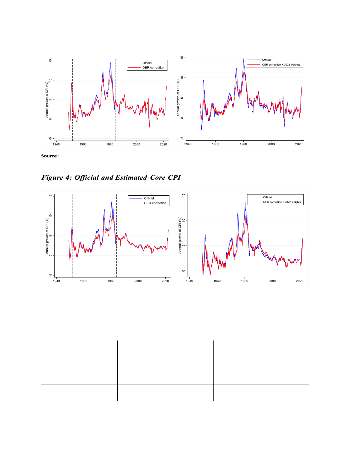
the official CPI data suggest. Figure 3 shows that the peak of the Volcker-era inflation (March
1980), currently understood to have been at 14.8 percent, is only 11.4 percent when adjusted
for the switch from homeownership costs to OER. The growth in core CPI at its peak in June
1980 falls from 13.6 percent to 9.1 percent when measured using the OER method as seen in
Figure 4. The large differences between the official and adjusted series reflect both the
substantial weight of OER in the index, especially in core CPI, and the lower peaks of estimated
OER relative to homeownership costs. From a low of 14.5 percent weight in 1983, as Americans
have shifted more of their consumption towards housing, OER has risen to represent 24.3
percent of overall CPI and 30.6 percent of core CPI in 2022. While past inflation peaks are lower
using the consistent methodology, the average inflation rate pre-1983 would also have been
lower. Our estimates show that the mean headline inflation rate between 1949 and 1983 is 0.4
percentage points lower when accounting for the shift to OER. lOMoAR cPSD| 46988474
Figure 3: Official and Estimated Headline CPI
Bureau of Labor Statistics, authors9 calculations
Notes: Percent change from 12 months earlier. Left-hand side: Homeownership costs are replaced with estimated OER pre-1983. Righthand side:
Homeownership costs are replaced with estimated OER pre-1983 and quantity weights are fixed at 2022 levels.
Source: Bureau of Labor Statistics, authors9 calculations
Notes: Percent change from 12 months earlier. Left-hand side: Homeownership costs are replaced with estimated OER pre-1983. Righthand side: Homeownership
costs are replaced with estimated OER pre-1983 and quantity weights are fixed at 2022 levels.
Table 1: Past Inflation Cycles and Today Headline CPI Core CPI Official Official Today9s Today9s Today9s Today9s Basis Basis and Basis Basis and weights weights -2.9 0.1 0.4 -0.2 0.3 1949-541 Start -2.9 14 lOMoAR cPSD| 46988474 Peak 9.4 9.4 3.3 7.2 6.9 5.0 End -0.7 -0.7 -0.5 -0.4 -0.4 -0.6 Reflation 12.3 12.3 3.2 6.8 7.1 4.7 Disinflation 10.1 10.1 3.8 7.6 7.3 5.6 1972-762 Start 2.7 2.4 2.2 2.8 2.2 2.1 Peak 12.3 11.0 9.1 11.7 9.5 7.8 End 4.9 5.1 5.9 6.1 6.3 6.1 Reflation 9.6 8.6 6.9 8.9 7.3 5.7 Disinflation 7.4 5.9 3.2 5.6 3.2 1.7 1978-833 Start 6.5 5.7 5.6 6.5 5.0 4.9 Peak 14.8 11.6 11.4 13.6 9.1 9.8 End 2.5 3.4 3.4 3.0 4.3 3.6 Reflation 8.3 5.9 5.8 6.1 4.1 4.9 Disinflation 12.3 8.2 8.0 10.6 4.8 6.2 Today11 Start 0.1 0.1 0.1 1.2 1.2 1.2 Peak 8.5 8.5 8.5 6.5 6.5 6.5 Reflation 8.4 8.4 8.4 5.3 5.3 5.3 Disinflation (to 6.5 6.5 6.5 4.5 4.5 4.5 2% target)
Sources: Bureau of Labor Statistics, Authors9 calculations
Notes: We define 8Start9 and 8End9 as the local minima of official annual headline CPI growth at the start and end of each cycle. We define 8Peak9
as the local maximum of official annual headline CPI and core CPI growth for each cycle. For official core CPI, we use the CPI less food series for the
period before 1958. Today9s basis: Homeownership costs are replaced with estimated OER pre-1983. Today9s basis and weights: Homeownership costs
are replaced with estimated OER pre-1983 and quantity weights are fixed at 2022 levels. 1
Start: July 1949. Peak: February 1951 for headline and June 1951 for core. End: October 1954. 2 Start: June 1972. Peak:
December 1974 for headline and February 1975 for core. End: December 1976. 3 Start: April 1978. Peak: March 1980 for
headline and June 1980 for core. End: July 1983.
More broadly speaking, past inflationary cycles would have been less volatile using the
consistent methodology that uses OER. The pace of reflation during the cycle upswings, and the
11 Start: May 2020. Peak: March 2022 for both headline and core. lOMoAR cPSD| 46988474
pace of disinflation during the cycle downswings are lower under today9s methodology, as
summarized in Table 1. These differences imply that the responsiveness of the CPI to monetary
policy was considerably lower during the 1960s and 1970s than the official CPI statistics suggest.
We stress that any consequences of the difference in measurement are larger for core CPI than
for headline CPI, due to the considerably larger weight of OER in core CPI.
Our estimates align with the retroactive CPI-U-RS series of the BLS that measures CPI inflation
consistently using current methods. Figure A.3 in the Appendix plots the CPI-U-RS series for
headline and core inflation, which overlap with our estimates for the period 1979-1983.
Whereas the CPI-U-RS series estimates the peak of headline inflation during the Volcker-era in
March 1980 at 11.8 percent, we estimate our peak in the same month at 11.6 percent. For core
inflation, both our adjusted series and the CPI-U-RS peak at 9.9 percent in December 1980, well
below the officially reported number of 12.2 percent for that month.
An alternative approach to making CPI more comparable is to attempt to apply pre-1983
techniques to this moment. This has been pursued Lee and Barton (2022), which extends work of
Hazell et al. (2020). After performing the complementary process, they also find that past and
present inflation look more similar than originally reported, with current levels higher than official
series due to the recent increase in mortgage rates.
Our estimates also indicate that past inflation cycles look more volatile than today9s due to the
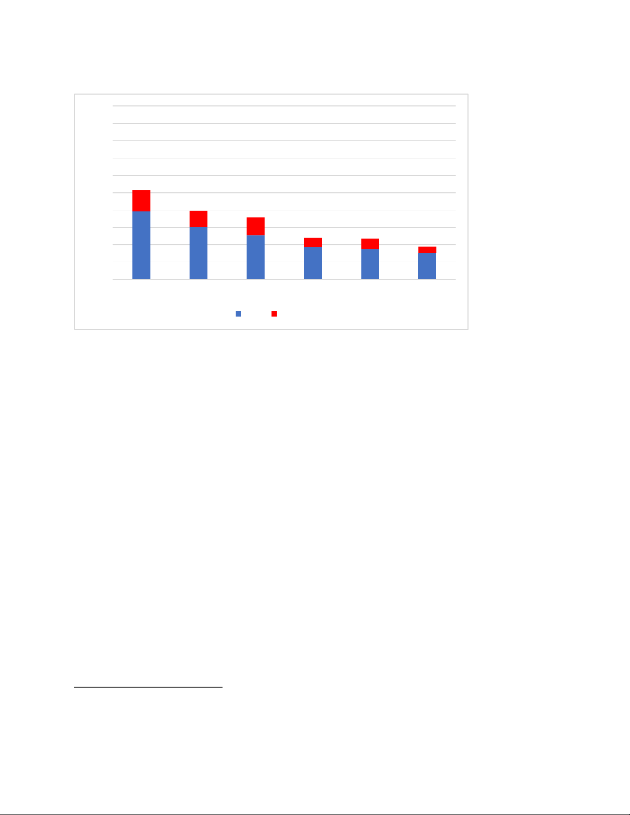
greater weight of transitory goods components in past measurements. In the early 1950s, for
example, food and apparel accounted for close to 50 percent of the headline CPI index (Figure
5). After the growth rate of these components shot above 10 percent due to Korean war-induced
shortages, headline inflation fell from 9 to 2 percent within a year. Today, however, food and 16 lOMoAR cPSD| 46988474
apparel only receive 17 percent of the weight of headline CPI. We estimate that the peak of
headline CPI inflation in 1951 would have been 3.3 percent, instead of 9.4 percent, when
measuring CPI using today9s weights. Our adjusted peak of core CPI inflation in 1951 is 5 percent,
compared to an official peak of 7.2 percent.
During the inflation cycle of the early 1970s, both the treatment of shelter inflation and the
greater weight of volatile goods components pushed up official CPI inflation compared to current
methods. When adjusting for the treatment of OER, our estimate of the peak of core CPI inflation
in February 1975 falls from 11.7 to 9.5 percent. We estimate that the peak of core CPI inflation in
1974 would have been only 7.8 percent when using today9s weights coupled with the
OER correction. The pre-Volcker adjusted trough was still 5.9 percent, suggesting the lessons
from the early 1970s for decreasing currently elevated inflation to around 2 percent are limited.
The index bears witness to this shift from transitory goods components to less volatile services,
with sticky industries gaining weight in the CPI across the board (Bryan and Meyer, 2010). The
current approach renders housing inflation particularly sticky (Bolhuis et al., 2022). Such
changes in measurement methods complicate comparisons between CPI rates from different
periods. By constructing CPI series using constant weights, we aim to improve the comparisons of CPI inflation over time. lOMoAR cPSD| 46988474
Figure 5: Average Food and Apparel Weight in Headline CPI by Revision 100% 90 % 80 % 70 % 60 % 50 % 40 % 30 % 20 % % 10 % 0 1946-1953 1954-1963 1964-1977 1978-1987 1988-1997 After 1997 Food Apparel
Source: Bureau of Labor Statistics, authors9 calculations
Note: Arithmetic mean of relative weight during each period.
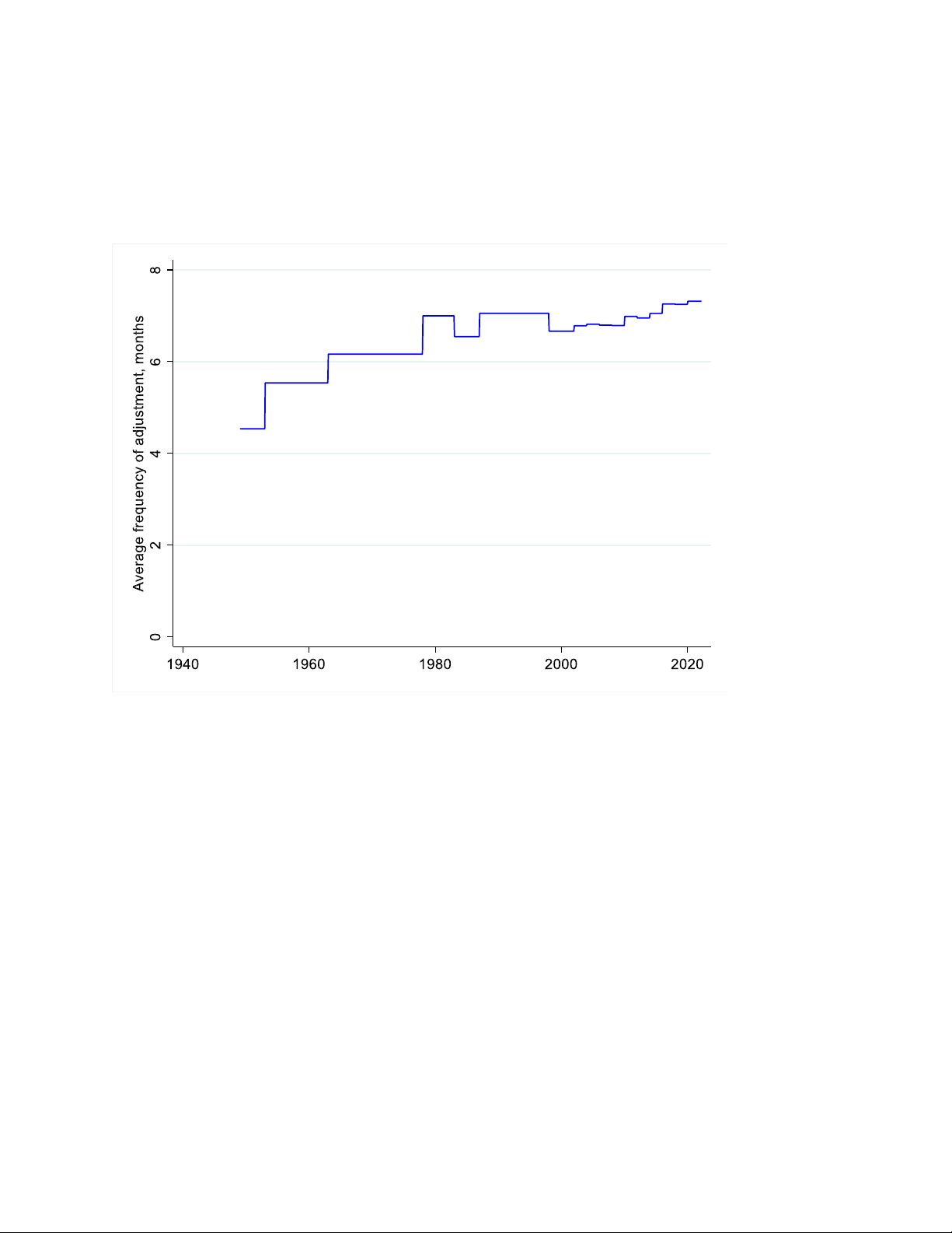
We formalize this shift towards sticky components of the CPI by constructing a time-varying
measure that reflects the average frequency of price adjustment, weighing each component by
its quantity weight. We take data on price adjustment from Bryan and Meyer (2010). Figure 6
plots the evolution of this measure over time. We estimate that the average frequency of price
adjustment has increased from 4.5 months in the late 1940s to 7.3 months in 2022. This secular
change is mainly driven by the increase in the weights of more sticky services components at
the expense of more transitory goods components such as food and apparel.12 12 18 lOMoAR cPSD| 46988474
Appendix Table A.2 contains the estimated frequency of adjustment from Bryan and Meyer (2010) by
component. Most food and apparel components have adjustment frequencies below five months, whereas the
frequency of price adjustment of most services components is above 10 months.
Figure 6: Average Frequency of Price Adjustment, Headline CPI Components
Source: Bureau of Labor Statistics, Bryan and Meyer (2010), authors9 calculations
Finally, we assess the implications of our new estimates of headline CPI inflation for real interest
rates and the monetary policy stance over time. Much has been made of the discrepancy
between high inflation and the low real monetary policy rate in the United States (e.g., Dudley,
2022). Recently, Blanchard (2022) emphasizes the similarities between the 1975-1983 inflation
cycle and the current one. During both inflationary upswings, the real federal funds rate
4measured as the nominal federal funds rate minus the annual core CPI inflation rate- has fallen
sharply below zero. And during both periods, a 8policy gap9 4measured as the difference