Solution for Linear Algebra
Tài liệu học tập môn Applied Linear Algebra tại Trường Đại học Quốc tế, Đại học Quốc gia Thành phố Hồ Chí Minh. Tài liệu gồm 203 trang giúp bạn ôn tập hiệu quả và đạt điểm cao! Mời bạn đọc đón xem!
Môn: Applied Linear Algebra 10 tài liệu
Trường: Trường Đại học Quốc tế, Đại học Quốc gia Thành phố Hồ Chí Minh 2 K tài liệu
Tác giả:


Preview text:
lOMoAR cPSD| 35974769
Instructor’s Solutions Manual Elementary Linear Algebra with Applications Ninth Edition Bernard Kolman Drexel University David R. Hill Temple University
Editorial Director, Computer Science, Engineering, and Advanced Mathematics: Marcia J. Horton Senior Editor: Holly Stark
Editorial Assistant: Jennifer Lonschein
Senior Managing Editor/Production Editor: Scott Disanno
Art Director: Juan Lo´pez
Cover Designer: Michael Fruhbeis
Art Editor: Thomas Benfatti
Manufacturing Buyer: Lisa McDowell
Marketing Manager: Tim Galligan
Cover Image: (c) William T. Williams, Artist, 1969 Trane, 1969 Acrylic on canvas, 108!! ×84!!.
Collection of The Studio Museum in Harlem. Gift of Charles Cowles, New York. lOMoAR cPSD| 35974769
"c 2008, 2004, 2000, 1996 by Pearson Education, Inc. Pearson Education, Inc.
Upper Saddle River, New Jersey 07458
Earlier editions "c 1991, 1986, 1982, by KTI; 1977, 1970 by Bernard Kolman
All rights reserved. No part of this book may be reproduced, in any form or by any means, without permission in writing from the publisher.
Printed in the United States of America 10 9 8 7 6 5 4 3 2 1 ISBN 0-13-229655-1
Pearson Education, Ltd., London
Pearson Education Australia PTY. Limited, Sydney Pearson
Education Singapore, Pte., Ltd
Pearson Education North Asia Ltd, Hong Kong
Pearson Education Canada, Ltd., Toronto Pearson
Educaci´on de Mexico, S.A. de C.V. Pearson
Education—Japan, Tokyo
Pearson Education Malaysia, Pte. Ltd Contents Preface iii
1 Linear Equations and Matrices 1
1.1 Systems of Linear Equations . . . . . . . . . . . . . . . . . . . . . . . . . . . . . . . . . . . . . 1
1.2 Matrices . . . . . . . . . . . . . . . . . . . . . . . . . . . . . . . . . . . . . . . . . . . . . . . . 2 1.3 Matrix Multiplication
. . . . . . . . . . . . . . . . . . . . . . . . . . . . . . . . . . . . . . . . 3
1.4 Algebraic Properties of Matrix Operations . . . . . . . . . . . . . . . . . . . . . . . . . . . . . 7
1.5 Special Types of Matrices and Partitioned Matrices . . . . . . . . . . . . . . . . . . . . . . . . 9 lOMoAR cPSD| 35974769
1.6 Matrix Transformations . . . . . . . . . . . . . . . . . . . . . . . . . . . . . . . . . . . . . . . 14
1.7 Computer Graphics . . . . . . . . . . . . . . . . . . . . . . . . . . . . . . . . . . . . . . . . . . 16
1.8 Correlation Coefficient . . . . . . . . . . . . . . . . . . . . . . . . . . . . . . . . . . . . . . . . 18
Supplementary Exercises . . . . . . . . . . . . . . . . . . . . . . . . . . . . . . . . . . . . . . . 19
Chapter Review . . . . . . . . . . . . . . . . . . . . . . . . . . . . . . . . . . . . . . . . . . . . 24
2 Solving Linear Systems 27
2.1 Echelon Form of a Matrix . . . . . . . . . . . . . . . . . . . . . . . . . . . . . . . . . . . . . . 27
2.2 Solving Linear Systems . . . . . . . . . . . . . . . . . . . . . . . . . . . . . . . . . . . . . . . . 28
2.3 Elementary Matrices; Finding A−1 . . . . . . . . . . . . . . . . . . . . . . . . . . . . . . . . . 30 2.4 Equivalent Matrices
. . . . . . . . . . . . . . . . . . . . . . . . . . . . . . . . . . . . . . . . . 32
2.5 LU-Factorization (Optional) . . . . . . . . . . . . . . . . . . . . . . . . . . . . . . . . . . . . . 33
Supplementary Exercises . . . . . . . . . . . . . . . . . . . . . . . . . . . . . . . . . . . . . . . 33
Chapter Review . . . . . . . . . . . . . . . . . . . . . . . . . . . . . . . . . . . . . . . . . . . . 35 3 Determinants 37
3.1 Definition . . . . . . . . . . . . . . . . . . . . . . . . . . . . . . . . . . . . . . . . . . . . . . . 37
3.2 Properties of Determinants . . . . . . . . . . . . . . . . . . . . . . . . . . . . . . . . . . . . . 37
3.3 Cofactor Expansion . . . . . . . . . . . . . . . . . . . . . . . . . . . . . . . . . . . . . . . . . . 39
3.4 Inverse of a Matrix . . . . . . . . . . . . . . . . . . . . . . . . . . . . . . . . . . . . . . . . . . 41
3.5 Other Applications of Determinants . . . . . . . . . . . . . . . . . . . . . . . . . . . . . . . . 42
Supplementary Exercises . . . . . . . . . . . . . . . . . . . . . . . . . . . . . . . . . . . . . . . 42
Chapter Review . . . . . . . . . . . . . . . . . . . . . . . . . . . . . . . . . . . . . . . . . . . . 43
4 Real Vector Spaces 45
4.1 Vectors in the Plane and in 3-Space . . . . . . . . . . . . . . . . . . . . . . . . . . . . . . . . 45
4.2 Vector Spaces . . . . . . . . . . . . . . . . . . . . . . . . . . . . . . . . . . . . . . . . . . . . . 47
4.3 Subspaces . . . . . . . . . . . . . . . . . . . . . . . . . . . . . . . . . . . . . . . . . . . . . . . 48
4.4 Span . . . . . . . . . . . . . . . . . . . . . . . . . . . . . . . . . . . . . . . . . . . . . . . . . . 51
4.5 Span and Linear Independence . . . . . . . . . . . . . . . . . . . . . . . . . . . . . . . . . . . 52
4.6 Basis and Dimension . . . . . . . . . . . . . . . . . . . . . . . . . . . . . . . . . . . . . . . . . 54
4.7 Homogeneous Systems . . . . . . . . . . . . . . . . . . . . . . . . . . . . . . . . . . . . . . . . 56
4.8 Coordinates and Isomorphisms . . . . . . . . . . . . . . . . . . . . . . . . . . . . . . . . . . . 58
4.9 Rank of a Matrix . . . . . . . . . . . . . . . . . . . . . . . . . . . . . . . . . . . . . . . . . . . 62 ii CONTENTS lOMoAR cPSD| 35974769
Supplementary Exercises . . . . . . . . . . . . . . . . . . . . . . . . . . . . . . . . . . . . . . . 64
Chapter Review . . . . . . . . . . . . . . . . . . . . . . . . . . . . . . . . . . . . . . . . . . . . 69 5 Inner Product Spaces 71
5.1 Standard Inner Product on R2 and R3 . . . . . . . . . . . . . . . . . . . . . . . . . . . . . . . 71
5.2 Cross Product in R3 (Optional) . . . . . . . . . . . . . . . . . . . . . . . . . . . . . . . . . . . 74
5.3 Inner Product Spaces . . . . . . . . . . . . . . . . . . . . . . . . . . . . . . . . . . . . . . . . . 77
5.4 Gram-Schmidt Process . . . . . . . . . . . . . . . . . . . . . . . . . . . . . . . . . . . . . . . . 81
5.5 Orthogonal Complements . . . . . . . . . . . . . . . . . . . . . . . . . . . . . . . . . . . . . . 84
5.6 Least Squares (Optional) . . . . . . . . . . . . . . . . . . . . . . . . . . . . . . . . . . . . . . 85
Supplementary Exercises . . . . . . . . . . . . . . . . . . . . . . . . . . . . . . . . . . . . . . . 86
Chapter Review . . . . . . . . . . . . . . . . . . . . . . . . . . . . . . . . . . . . . . . . . . . . 90
6 Linear Transformations and Matrices 93
6.1 Definition and Examples . . . . . . . . . . . . . . . . . . . . . . . . . . . . . . . . . . . . . . . 93
6.2 Kernel and Range of a Linear Transformation . . . . . . . . . . . . . . . . . . . . . . . . . . . 96
6.3 Matrix of a Linear Transformation . . . . . . . . . . . . . . . . . . . . . . . . . . . . . . . . . 97
6.4 Vector Space of Matrices and Vector Space of Linear Transformations (Optional) . . . . . . . 99
6.5 Similarity . . . . . . . . . . . . . . . . . . . . . . . . . . . . . . . . . . . . . . . . . . . . . . . 102
6.6 Introduction to Homogeneous Coordinates (Optional) . . . . . . . . . . . . . . . . . . . . . . 103 Supplementary
Exercises . . . . . . . . . . . . . . . . . . . . . . . . . . . . . . . . . . . . . . . 105
Chapter Review . . . . . . . . . . . . . . . . . . . . . . . . . . . . . . . . . . . . . . . . . . . . 106
7 Eigenvalues and Eigenvectors 109
7.1 Eigenvalues and Eigenvectors . . . . . . . . . . . . . . . . . . . . . . . . . . . . . . . . . . . . 109
7.2 Diagonalization and Similar Matrices . . . . . . . . . . . . . . . . . . . . . . . . . . . . . . . . 115
7.3 Diagonalization of Symmetric Matrices . . . . . . . . . . . . . . . . . . . . . . . . . . . . . . . 120 Supplementary
Exercises . . . . . . . . . . . . . . . . . . . . . . . . . . . . . . . . . . . . . . . 123
Chapter Review . . . . . . . . . . . . . . . . . . . . . . . . . . . . . . . . . . . . . . . . . . . . 126
8 Applications of Eigenvalues and Eigenvectors (Optional) 129
8.1 Stable Age Distribution in a Population; Markov Processes . . . . . . . . . . . . . . . . . . . 129
8.2 Spectral Decomposition and Singular Value Decomposition
. . . . . . . . . . . . . . . . . . . 130
8.3 Dominant Eigenvalue and Principal Component Analysis . . . . . . . . . . . . . . . . . . . . 130
8.4 Differential Equations . . . . . . . . . . . . . . . . . . . . . . . . . . . . . . . . . . . . . . . . 131
8.5 Dynamical Systems . . . . . . . . . . . . . . . . . . . . . . . . . . . . . . . . . . . . . . . . . . 132
8.6 Real Quadratic Forms . . . . . . . . . . . . . . . . . . . . . . . . . . . . . . . . . . . . . . . . 133
8.7 Conic Sections . . . . . . . . . . . . . . . . . . . . . . . . . . . . . . . . . . . . . . . . . . . . 134
8.8 Quadric Surfaces . . . . . . . . . . . . . . . . . . . . . . . . . . . . . . . . . . . . . . . . . . . 135 10 MATLAB Exercises 137
Appendix B Complex Numbers 163
B.1 Complex Numbers . . . . . . . . . . . . . . . . . . . . . . . . . . . . . . . . . . . . . . . . . . 163 lOMoAR cPSD| 35974769
B.2 Complex Numbers in Linear Algebra . . . . . . . . . . . . . . . . . . . . . . . . . . . . . . . . 165 Preface
This manual is to accompany the Ninth Edition of Bernard Kolman and David R.Hill’s Elementary Linear Algebra
with Applications. Answers to all even numbered exercises and detailed solutions to all theoretical exercises are
included. It was prepared by Dennis Kletzing, Stetson University. It contains many of the solutions found in the
Eighth Edition, as well as solutions to new exercises included in the Ninth Edition of the text. lOMoAR cPSD| 35974769 Chapter 1
Linear Equations and Matrices Section 1.1, p. 8
2. x = 1, y = 2, z = −2. 4. No solution.
6. x = 13 + 10t, y = −8 − 8t, t any real number. 8. Inconsistent; no solution.
10. x = 2, y = −1. 12. No solution. 14. x = 1, y = 2, z = 2. 16. (a) For example: = 0
is one answer. (b) For example: s = 3, t = 4 is one answer. .
18. Yes. The trivial solution is always a solution to a homogeneous system.
20. x = 1, y = 1, z = 4. 22. r = −3.
24. If x1 = s1, x2 = s2, ..., xn = sn satisfy each equation of (2) in the original order, then those same numbers
satisfy each equation of (2) when the equations are listed with one of the original ones interchanged, and conversely.
25. If x1 = s1, x2 = s2, ..., xn = sn is a solution to (2), then the pth and qth equations are satisfied. That is, .
Thus, for any real number r,
(ap1 + raq1)s1 + ··· + (apn + raqn)sn = bp + rbq.
Then if the qth equation in (2) is replaced by the preceding equation, the values x1 = s1, x2 = s2, ..., xn = sn are
a solution to the new linear system since they satisfy each of the equations. lOMoAR cPSD| 35974769 2 Chapter 1 26. (a) A unique point.
(b) There are infinitely many points.
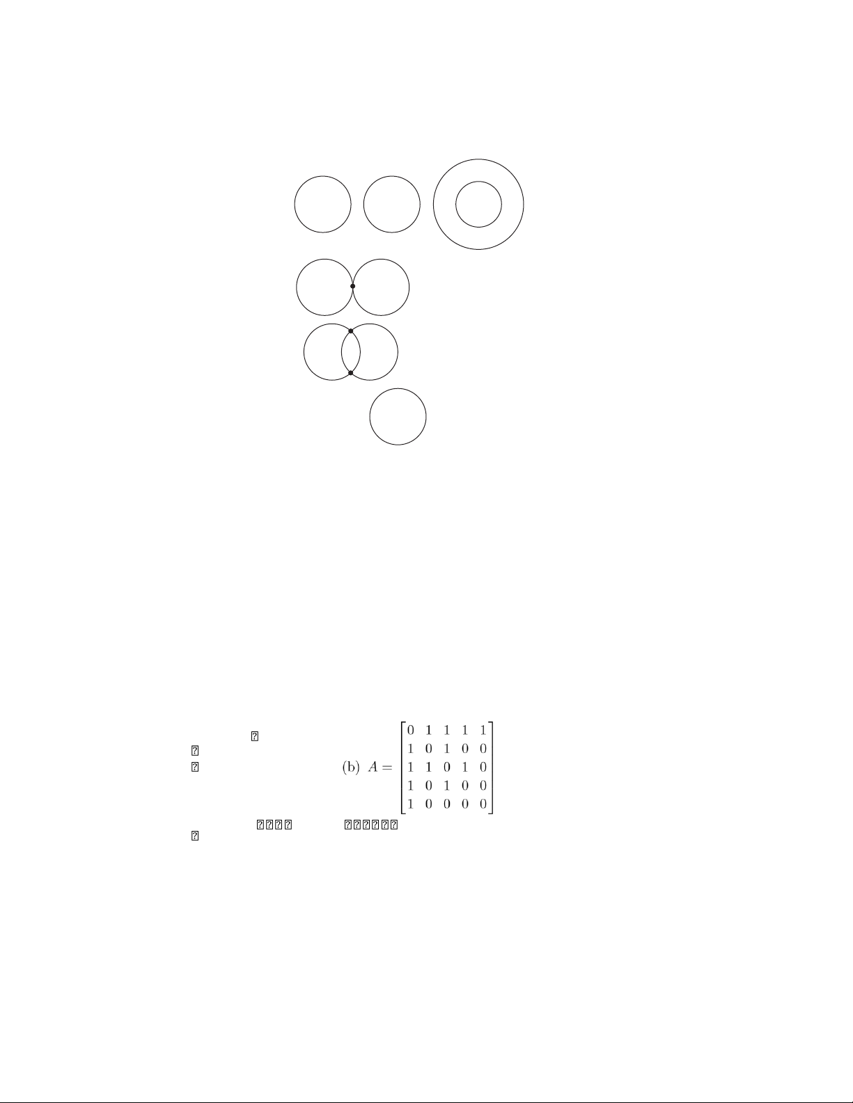
(c) No points simultaneously lie in all three planes. C 2
28. No points of intersection: C 1 C 2 C 1 One point of C 1 C 2 intersection: C 1 C 2 Two points of intersection: C 1 = C 2 Infinitely many points of intersection:
30. 20 tons of low-sulfur fuel, 20 tons of high-sulfur fuel.
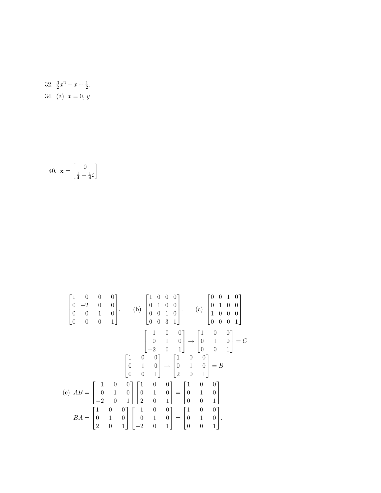
32. 3.2 ounces of food A, 4.2 ounces of food B, and 2 ounces of food C. 34.
(a) p(1) = a(1)22 + b(1) + c = a + b + c = −5
p(−1) = a(−1)2 + b(−1) + c = a − b + c = 1 p(2) =
a(2) + b(2) + c = 4a + 2b + c = 7.
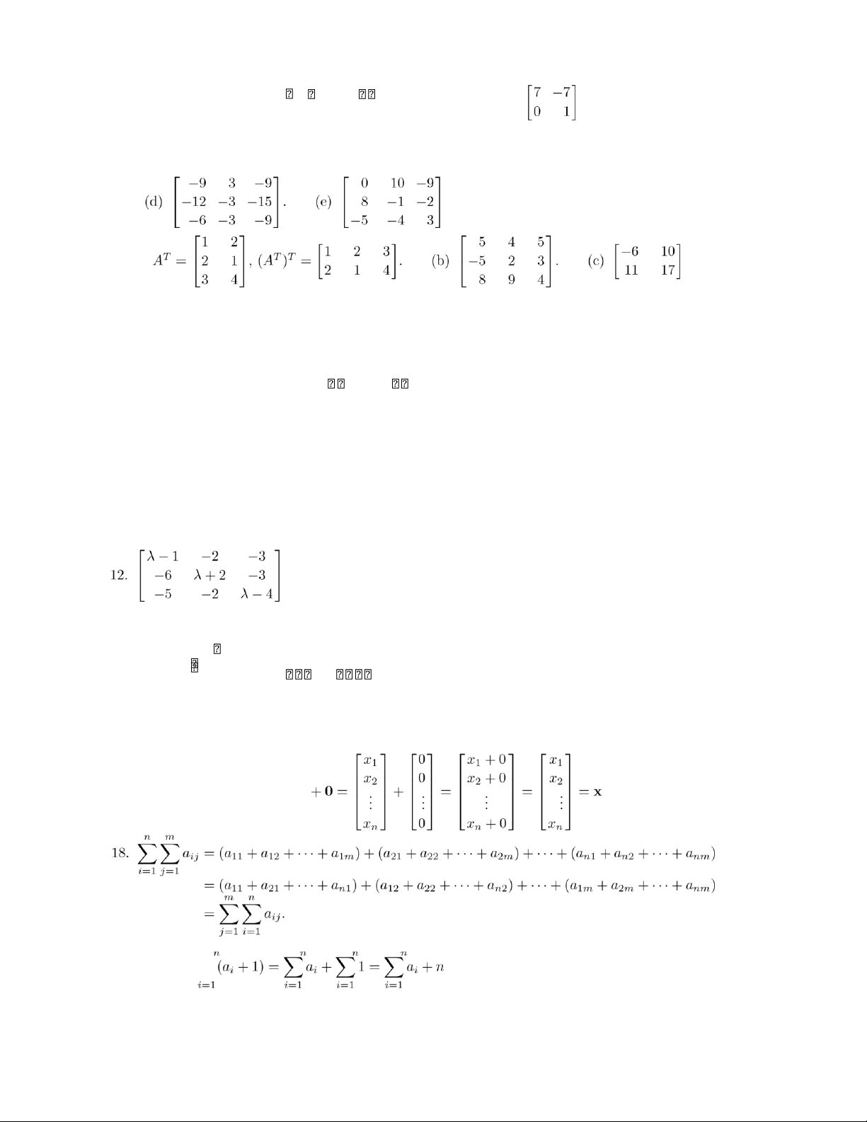
(b) a = 5, b = −3, c = −7. Section 1.2, p. 19 0 1 0 0 1 1 0 1 1 1 2. (a) A = 0 1 0 0 0 . 0 1 0 0 0 1 1 0 0 0
4. a = 3, b = 1, c = 8, d = −2. lOMoAR cPSD| 35974769 3 5 −5 8 6.
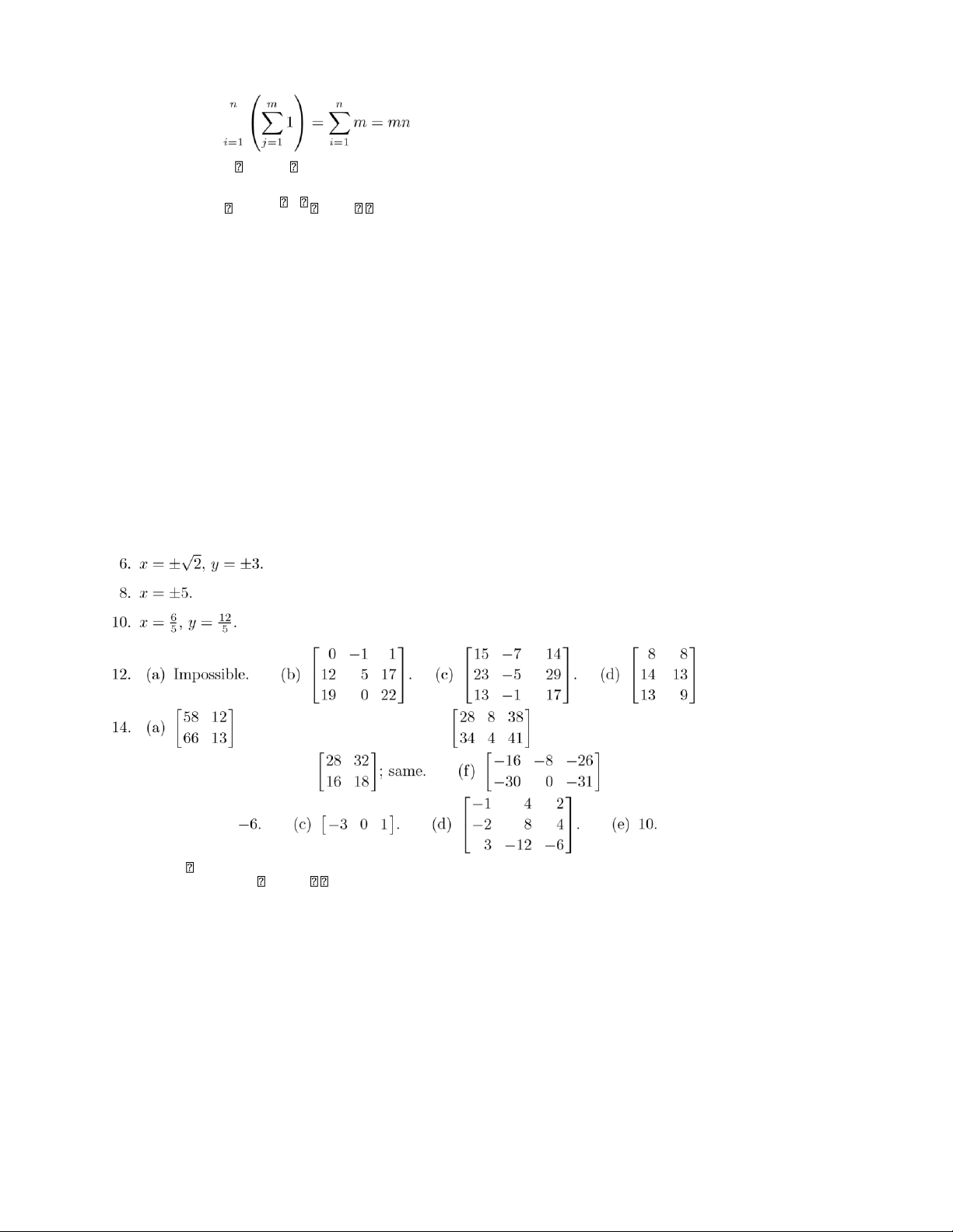
(a) C + E = E + C =4 2 9 . (b) Impossible. (c) . 5 3 4 . (f) Impossible. 8. ( a) . Section 1.3 ' 3 4 0 (d)−4(. (e) 6 3 . (f) ' 17 2(. 4 0 9 10 −16 6 1 0 1 0 3 0 '10. Y es: 2( + 1' ( = ' (. 0 1 0 0 0 2 .
14. Because the edges can be traversed in either direction. x1 16. Let x = ...2
be an n-vector. Then x xn x . 19. (a) True. ) . lOMoAR cPSD| 35974769 4 Chapter 1 (b) True. ) . (c) True. )i=1 ai )j=1 bj
= a1)j=1 bj + a2)j=1 bj + ··· + an)j=1 bj n m m m m m
= (a1 + a2 + ··· + an))j=1 bj n m m n
= )ai )bj = ).)aibj/ i=1 j=1 j=1 i=1
20. “new salaries” = u + .08u = 1.08u. Section 1.3, p. 30 2. (a) 4. (b) 0. (c) 1. (d) 1. 4. x = 5. . (e) Impossible. . (b) Same as (a). ( c) . (d) Same as (c). ( e) . 16. (a) 1. ( b) 9 0 −3 (f)0 0 0 . (g) Impossible. −3 0 1
18. DI2 = I2D = D. 0 0 ' 20.(. 0 0 lOMoAR cPSD| 35974769 5 1 0 14 18 0 3 22. (a). (b) . 13 13 11 −2 −1 2 1 −2 −1 24. col (AB) = 1 2 + 3 4
+ 2 3 ; col (AB) = −1 2 + 2 4 + 4 3 . 3 0 −2 3 0 −2 26. (a) −5. (b) BAT
28. Let A = 0aij1 be m × p and B = 0bij1 be p × n. ik
(a) Let the ith row of A consist entirely of zeros, so that a = 0 for k = 1,2,. .,p. Then the (i,j) entry in AB is )= 0
for j = 1,2,...,n.
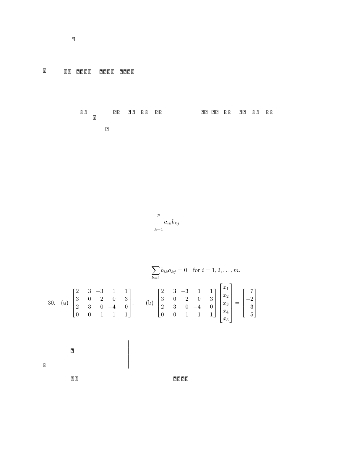
(b) Let the jth column of A consist entirely of zeros, so that akj = 0 for k = 1,2,...,m. Then the (i,j) entry in BA is m . Section 1.3 2 3 −3 1 17 (c) 23 30 021 −401 031−253 0 0 lOMoAR cPSD| 35974769 6 Chapter 1 32. '−2 3('x12( = '5(. 1 −5 x 4
2x1 + x2 + 3x3 + 4x4 = 0 34. (a)
3x1 − x2 + 2x3 = 3 (b) same as (a).
−2x1 + x2 − 4x3 + 3x4 = 2 ' 13( 2 ' 2( 3 '1( ' 4( 1 −1 2 1 3
36. (a) x1 + x −1 + x 4 = −2 .
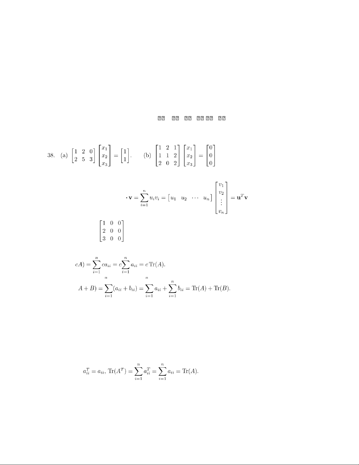
(b) x 32 + x −11 = −21 . . 39. We have u . 40. Possible answer: . 42. (a) Can say nothing. (b) Can say nothing. 43. (a) Tr( (b) Tr(
(c) Let AB = C = 0cij1. Then n n n n n
Tr(AB) = Tr(C) = )cii = ))aikbki = ))bkiaik = Tr(BA). i=1 i=1 k=1 k=1 i=1 (d) Since
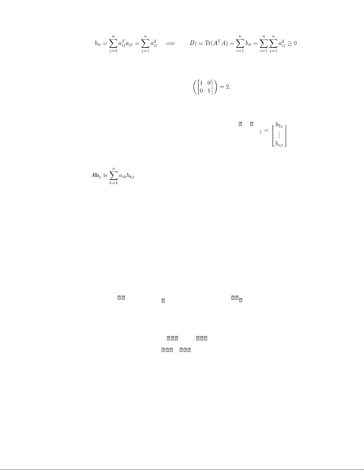
(e) Let ATA = B = 0bij1. Then lOMoAR cPSD| 35974769 7 Tr( . Hence, Tr(ATA) ≥ 0. 44. (a) 4. (b) 1. (c) 3.
45. We have Tr(AB − BA) = Tr(AB) − Tr(BA) = 0, while Tr ij ij b1j
46. (a) Let A = 0a 1 and B = 0b 1 be m × n and n × p, respectively. Then band the ith entry of
, which is exactly the (i,j) entry of AB. (b) ···
The ith row of AB is 04k aikbk1 4k aikbk2
4k aikbkn1. Since ai = 0ai1 ai2 ··· ain1, we have aib = 04k aikbk1
4k aikbk2 ··· 4k aikbkn1.
This is the same as the ith row of Ab.
47. Let A = 0aij1 and B = 0bij1 be m × n and n × p, respectively. Then the jth column of AB is (AB)j =
am111b11jj +
···... + a1mnnbnj
a b + ··· + a bnj = b1j m11... 1 + ··· + bnj ... a a1n a amn
= b1jCol1(A) + ··· + bnjColn(A).
Thus the jth column of AB is a linear combination of the columns of A with coefficients the entries in bj.
48. The value of the inventory of the four types of items.
50. (a) row1(A) · col1(B) = 80(20) + 120(10) = 2800 grams of protein consumed daily by the males. lOMoAR cPSD| 35974769 8 Chapter 1
(b) row2(A) · col2(B) = 100(20) + 200(20) = 6000 grams of fat consumed daily by the females.
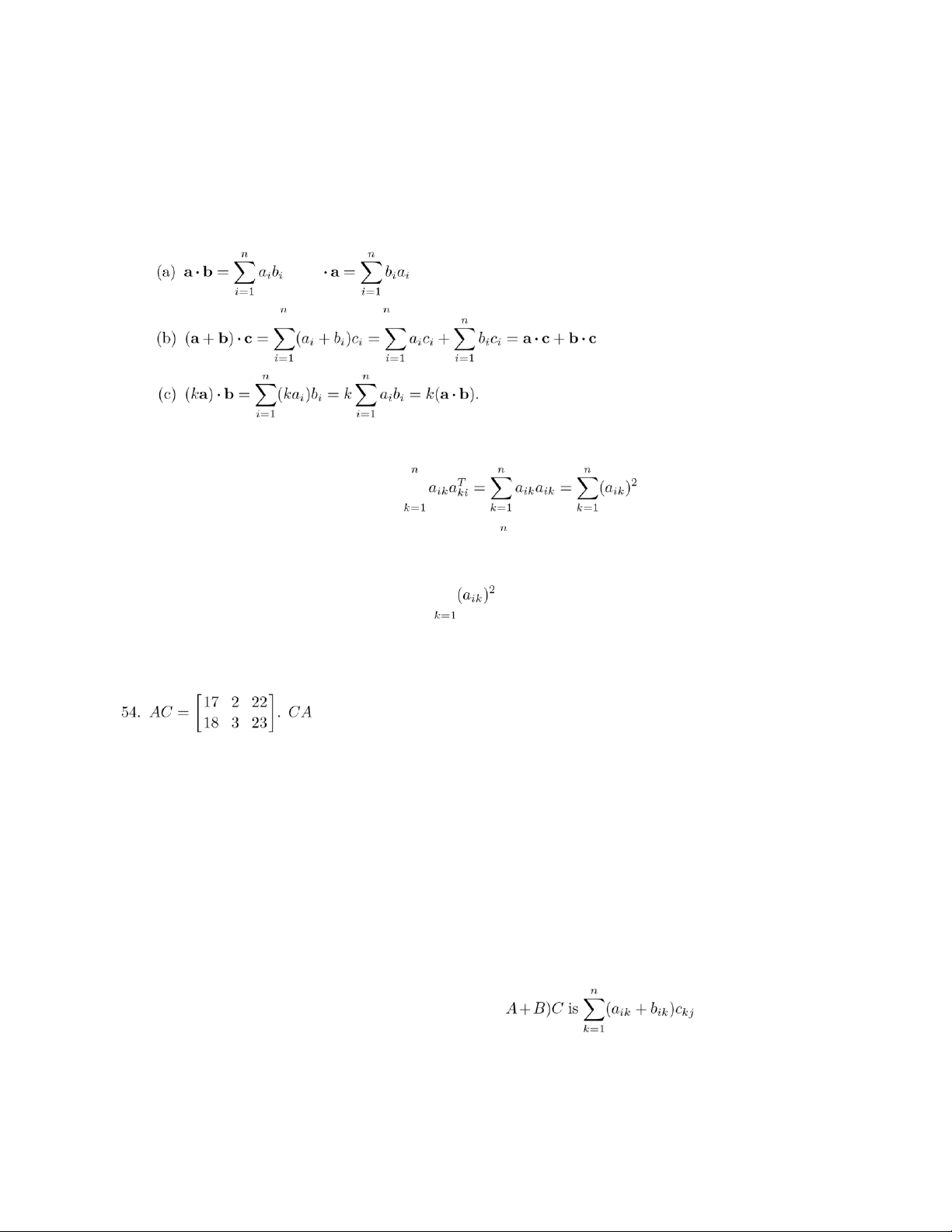
51. (a) No. If x = (x1,x2,...,xn), then x·x = x21 + x22 + ··· + x2n ≥ 0. (b) x = 0.
52. Let a = (a1,a2,. .,an), b = (b1,b2,. .,bn), and c = (c1,c2,. .,cn). Then and b
, so a·b = b·a. . Section 1.4
53. The i, ith element of the matrix AAT is ) .
Thus if AAT = O, then each sum of squares
) equals zero, which implies aik = 0 for each i and k. Thus A = O. cannot be computed.
55. BTB will be 6 × 6 while BBT is 1 × 1. Section 1.4, p. 40
1. Let A = 0aij1, B = 0bijij1, C ij= 0cijij1. Then the (i,j) entry of A + (B + C) is aij + (bij + cij) and that of (A + B) + C
is (a + b ) + c . By the associative law for addition of real numbers, these two entries are equal.
2. For A = 0aij1, let B = 0−aij1.
4. Let A = 0aij1, B = 0bij1, C = 0cij1. Then the (i,j) entry of ( and that of lOMoAR cPSD| 35974769 9
. By the distributive and additive associative laws for real numbers,
these two expressions for the (i,j) entry are equal.
, where aii = k and aij = 0 if i & = j, and let
. Then, if i &= j, the (i,j) entry of
, while if i = j, the (i,i) entry of
. Therefore AB = kB.
7. Let A = 0aij1 and C = 0c1 c2
··· cm1. Then CA is a 1 × n matrix whose ith entry is ) . a1j Sinceth entry of ) . 8. (a). − − −
(d) The result is true for p = 2 and 3 as shown in parts (a) and (b). Assume that it is true for p = k. Then coskθ sinkθ cosθ sinθ Ak+1 = AkA = ' (' (
−sinkθ coskθ −sinθ cosθ = '
coskθ cosθ − sinkθsinθ coskθ sinθ + sinkθ cosθ(
−sinkθ cosθ − coskθ sinθ coskθ cosθ − sinkθ sinθ
= ' (. cos(k + 1)θ sin(k + 1)θ
−sin(k + 1)θ cos(k + 1)θ Hence, it is
true for all positive integers k. 10. Possible answers:. 12. Possible answers:.
13. Let A = 0aij1. The (i,j) entry of r(sA) is r(saij), which equals (rs)aij and s(raij). lOMoAR cPSD| 35974769 10 Chapter 1 14. Let A =
aij . The (i,j) entry of (r + s)A is (r + s)aij, which equals raij + saij, the (i,j) entry of rA + sA.0 1
16. Let A = 0aij1, and B = 0bij1. Then r(aij + bij) = raij + rbij.
18. Let A = 0aij1 and B = 0bij1. The (i,j) entry of), which equals, the
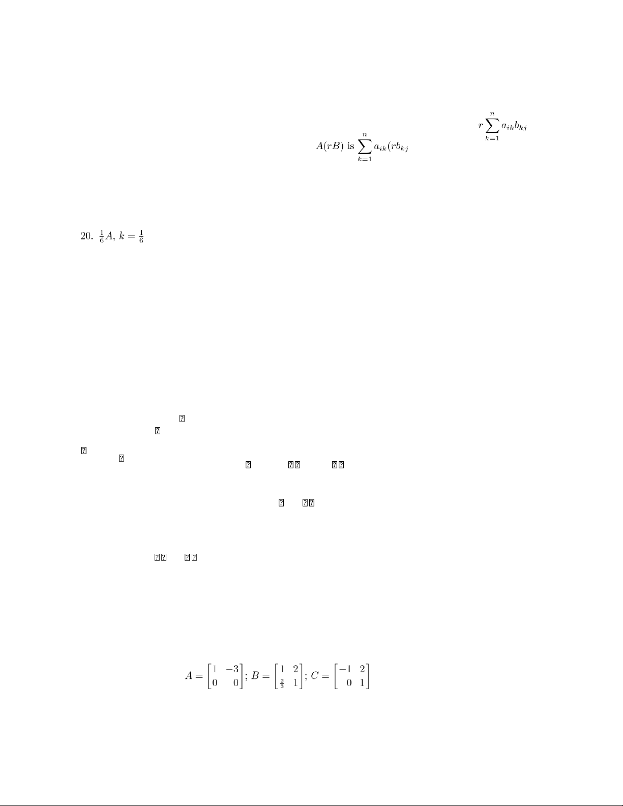
(i,j) entry of r(AB). . 22. 3.
24. If Ax = rx and y = sx, then Ay = A(sx) = s(Ax) = s(rx) = r(sx) = ry.
26. The (i,j) entry of (AT)T is the (j,i) entry of AT, which is the (i,j) entry of A.
27. (b) The (i,j) entry of (A + B) is the (j,i) entry of a + b , which is to say, a + b .
(d) Let A = 0aijij1 and let bij =T aji. Then the (i,j) entry of0 ij
ij(cA1 )T is the (j,i) entry ofji ji0caij1, which is to say, cb . 5 0 −4 −8
28. (A + B)T =5 2 , (rA)T = −12 −4 . 1 2 −8 12 −51 −51 T −34−34 30. (a)17 . (b) 17 .
(c) B C is a real number (a 1 × 1 matrix). 32. Possible answers: . lOMoAR cPSD| 35974769 11 .
33. The (i,j) entry of cA is caij, which is 0 for all i and j only if c = 0 or aij = 0 for all i and j. 34. Let
( be such that AB = BA for any 2 × 2 matrix B. Then in particular, ' (' ( = ' (' (
a b 1 0 1 0 a b c d 0 0 ' 0 0 c d ( = ' ( a 0 a b c 0 0 0 so . lOMoAR cPSD| 35974769 12 Chapter 1 Also ' (' ( = ' (' (
a 0 1 1 1 1 a 0 0 d 0 0 ' 0 0 0 d ( = ' (, a a a d 0 0 0 0
which implies that a = d. Thus ( for some number a. 35. We have
(A − B)T = (AT+ (−1)B)T
= AT + ((−1)BT)T T T = A + (−1)B = A − B by Theorem 1.4(d)).
36. (a) A(x1 + x2) = Ax1 + Ax2 = 0 + 0 = 0. (b) A(x1 − x2) = Ax1 − Ax2 = 0 − 0 = 0.
(c) A(rx1) = r(Ax1) = r0 = 0.
(d) A(rx1 + sx2) = r(Ax1) + s(Ax2) = r0 + s0 = 0.
37. We verify that x3 is also a solution:
Ax3 = A(rx1 + sx2) = rAx1 + sAx2 = rb + sb = (r + s)b = b.
38. If Ax1 = b and Ax2 = b, then A(x1 − x2) = Ax1 − Ax2 = b − b = 0. Section 1.5, p. 52
1. (a) Let Im = 0dij1 so dij = 1 if i = j and 0 otherwise. Then the (i,j) entry of ImA is )
(since all other d’s = 0) = aij (since dii = 1).
2. We prove that the product of two upper triangular matrices is upper triangular: Let with aij =
0 for i > j; let B = 0bij1 with bij = 0 for i > jik . Then AB = 0cij1 where kj . For lOMoAR cPSD| 35974769 Section 1.5 13
i > j, and each 1 ≤ckij≤is 0 and son, either i > kcij = 0(. Henceand so a0cij= 0)1 is upper triangular.or else k
≥ i > j (so b = 0). Thus every term in the sum for 3. Let
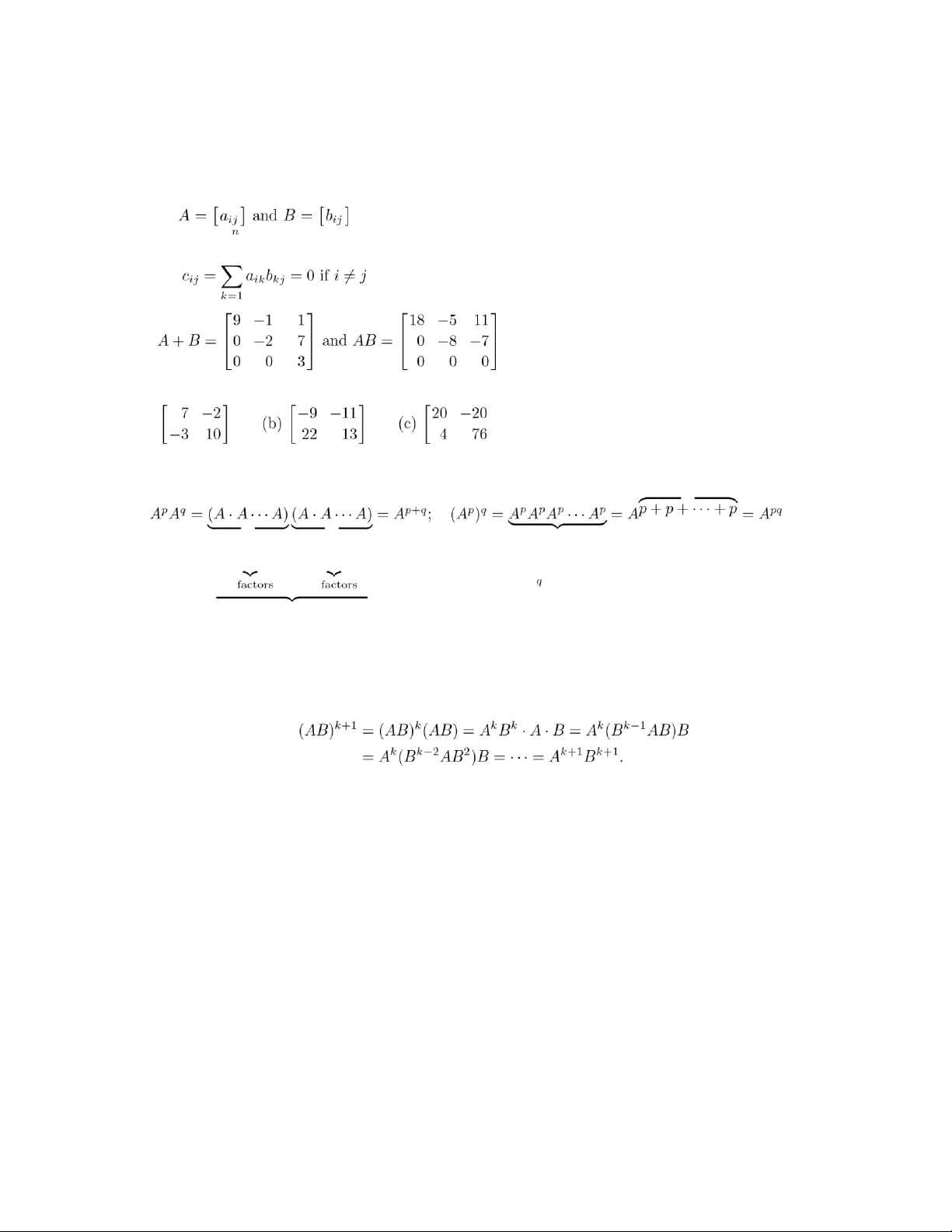
, where both aij = 0 and bij = 0 if i =& j. Then if AB = C = 0cij1, we have . 4. . 5. All diagonal matrices. 6. ( a) ( q summands 8. 85 . p q factors 5 p + q factors 8
9. We are given that AB = BA. For p = 2, (AB)2 = (AB)(AB) = A(BA)B = A(AB)B = A2B2. Assume that for p = k,
(AB)k = AkBk. Then
Thus the result is true for p = k + 1. Hence it is true for all positive integers p. For p = 0, (AB)0 = In = A0B0.
10. For p = 0, (cA)0 = In = 1 · In = c0 · A0. For p = 1, cA = cA. Assume the result is true for p = k: (cA)k = ckAk, then for k + 1:
(cA)k+1 = (cA)k(cA) = ckAk · cA = ck(Akc)A = ck(cAk)A = (ckc)(AkA) = ck+1Ak+1.
11. True for p = 0: (AT)0 = In = InT = (A0)T. Assume true for p = n. Then
(AT)n+1 = (AT)nAT = (An)TAT = (AAn)T = (An+1)T.
12. True for p = 0: (A0)−1 = In−1 = In. Assume true for p = n. Then
(An+1)−1 = (AnA)−1 = A−1(An)−1 = A−1(A−1)n = (A−1)n+1. lOMoAR cPSD| 35974769 14 Chapter 1 and ( . Hence, ( for
14. (a) Let A = kIn. Then AT = (kIn)T = kInT = kIn = A.
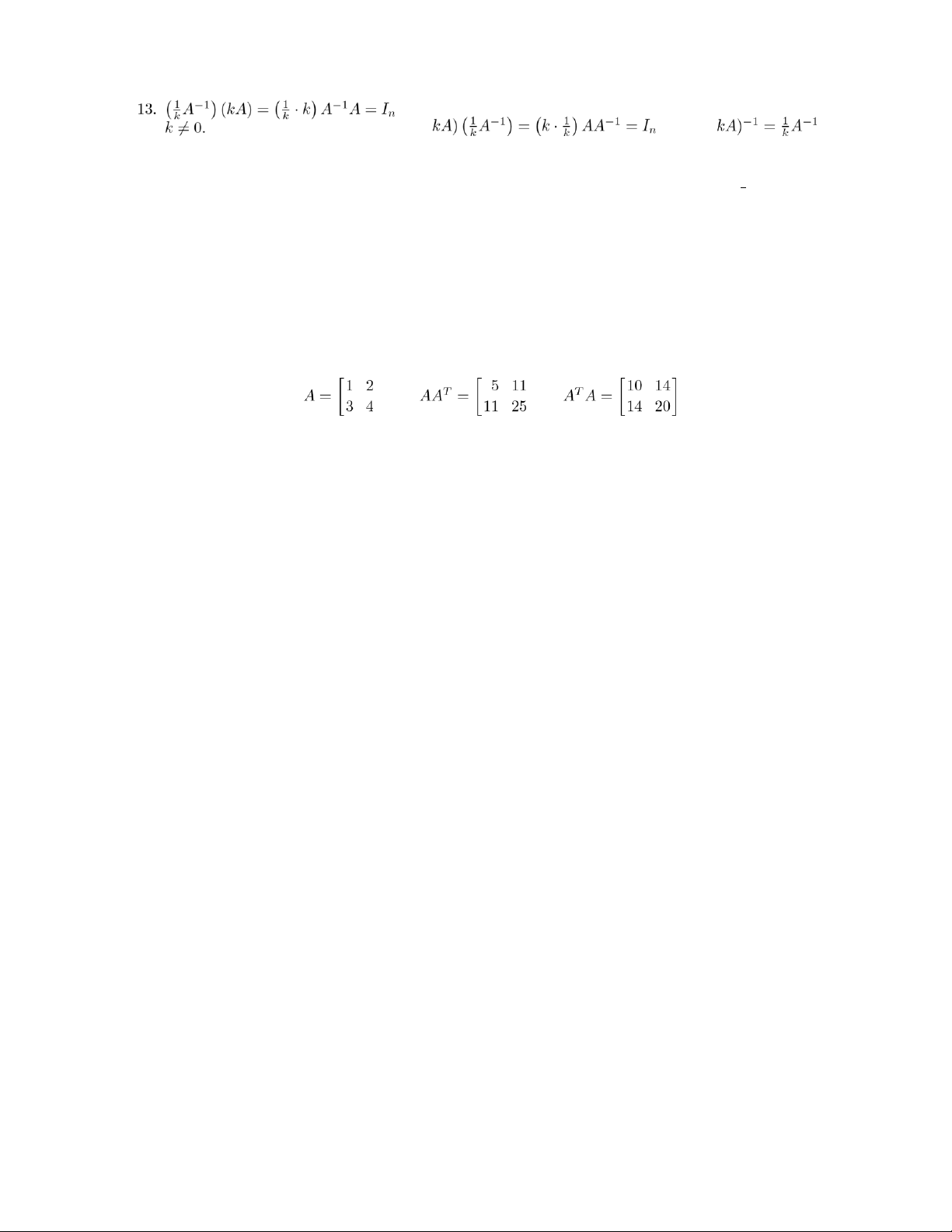
(b) If k = 0, then A = kIn = 0In = O, which is singular. If k &= 0 , then A−1 = (kA)−1 = k1A−1, so A is nonsingular.
(c) No, the entries on the main diagonal do not have to be the same. a b
' 16. Possible answers:(. Infinitely many. 0 a 17. The result is false. Let (. Then ( and .
18. (a) A is symmetric if and only if AT = A, or if and only if aij = aTij = aji.
(b) A is skew symmetric if and only if AT = −A, or if and only if aTij = aji = −aij.
(c) aii = −aii, so aii = 0.
19. Since A is symmetric, AT = A and so (AT)T = AT. 20. The zero matrix.
21. (AAT)T = (AT)TAT = AAT.
22. (a) (A + AT)T = AT + (AT)T = AT + A = A + AT.
(b) (A − AT)T = AT − (AT)T = AT − A = −(A − AT).
23. (Ak)T = (AT)k = Ak.
24. (a) (A + B)T = AT + BT = A + B.
(b) If AB is symmetric, then (AB)T = AB, but (AB)T = BTAT = BA, so AB = BA. Conversely, if AB = BA, then
(AB)T = BTAT = BA = AB, so AB is symmetric.
25. (a) Let A = 0aij1 be upper triangular, so that aij = 0 for i > j. Since AT = 0aijT1, where aTij = aji, we have aTij =
0 for j > i, or aTij = 0 for i < j. Hence AT is lower triangular.
(b) Proof is similar to that for (a).
26. Skew symmetric. To show this, let A be a skew symmetric matrix. Then AT = −A. Therefore (AT)T = A = −AT.
Hence AT is skew symmetric. lOMoAR cPSD| 35974769 Section 1.5 15
27. If A is skew symmetric, AT = −A. Thus aii = −aii, so aii = 0.
28. Suppose that A is skew symmetric, so AT = −A. Then (Ak)T = (AT)k = (−A)k = −Ak if k is a positive odd integer,
so Ak is skew symmetric.
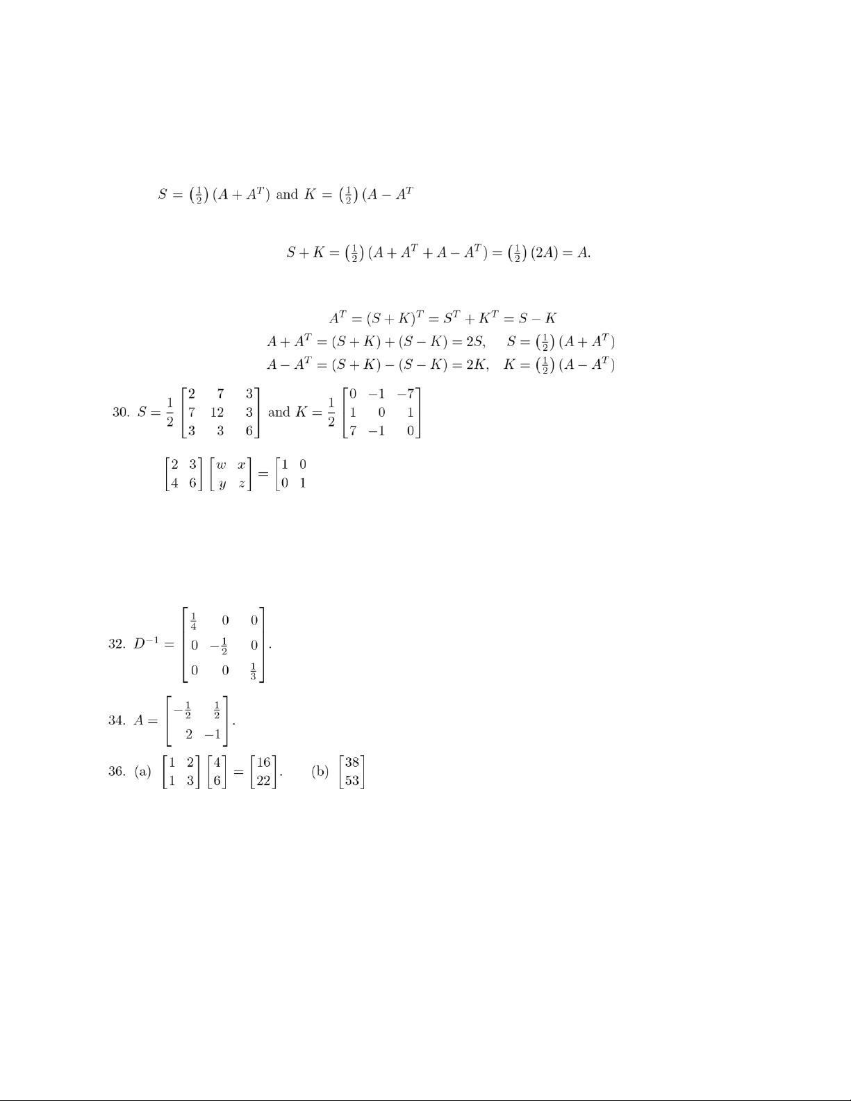
29. Let). Then S is symmetric and K is skew symmetric, by Exercise 18. Thus
Conversely, suppose A = S + K is any decomposition of A into the sum of a symmetric and skew symmetric matrix. Then , . 31. Form (. Since the linear systems
2w + 3y = 1 2x + 3z = 0 and 4w + 6y = 0 4x + 6z = 1
have no solutions, we conclude that the given matrix is singular. . lOMoAR cPSD| 35974769 Chapter 1 . 42. Possible answer: . 43. Possible answer: .
44. The conclusion of the corollary is true forconclusion is true for a sequence of r − 1 matrices. Thenr = 2, by Theorem 1.6.
Suppose r ≥ 3 and that the .
45. We have A−1A = In = AA−1 and since inverses are unique, we conclude that (A−1)−1 = A.
46. Assume that A is nonsingular, so that there exists an n×n matrix B such that AB = In. Exercise 28AB = In. in
Section 1.3 implies that AB has a row consisting entirely of zeros. Hence, we cannot have 47. Let , where aii = 0&
for i = 1,2,. .,n. Then as can be verified by computing 16 0 0 48. A4 = 0 81 0 . 0 0 625 lOMoAR cPSD| 35974769 Section 1.5 17 ap110p22 0 ··· 0 49. Ap = 0 a 0... ··· 0 . 0 0 ··· ··· apnn
50. Multiply both sides of the equation by A−1.
51. Multiply both sides by A−1. 52. Form
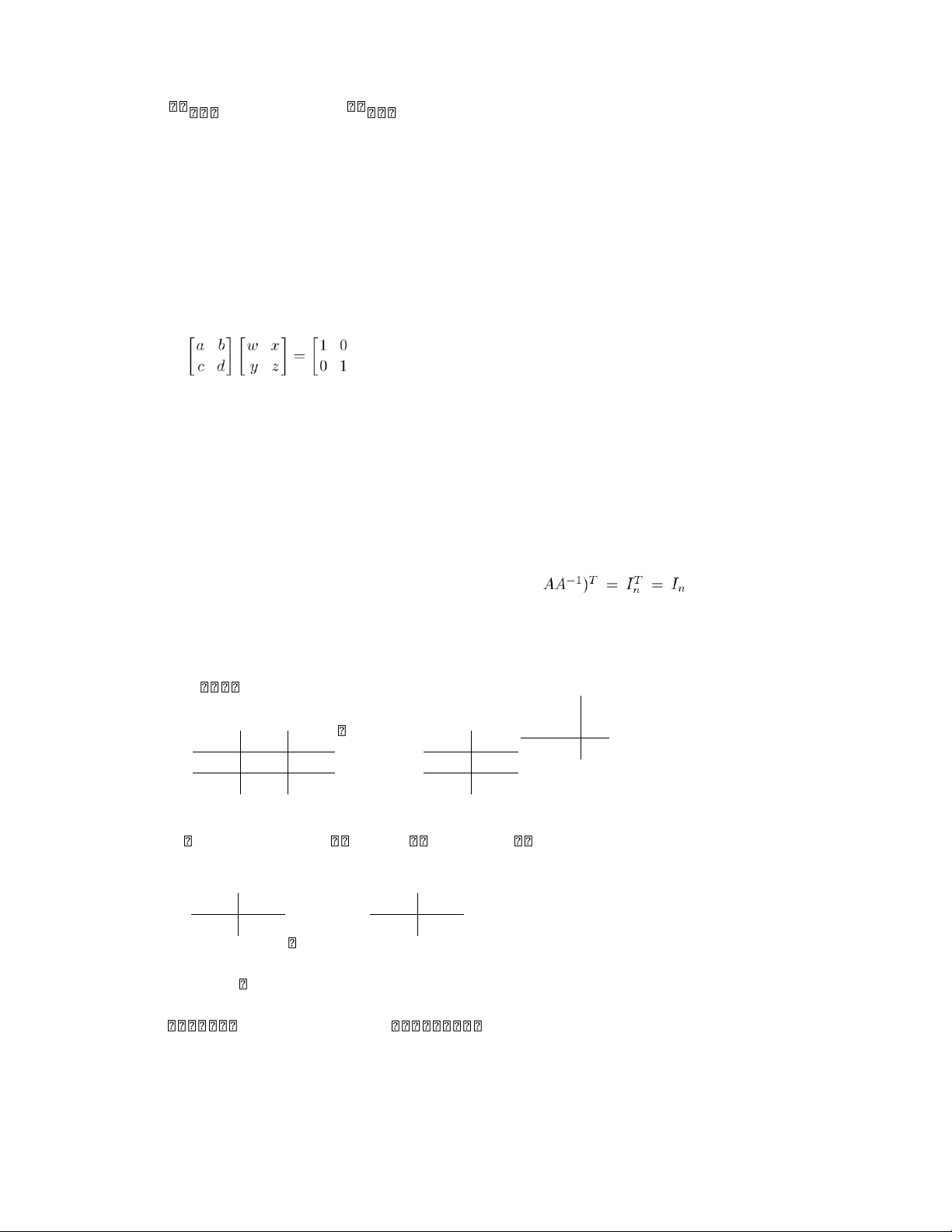
(. This leads to the linear systems aw + by = 1 ax + bz = 0
and cw + dy = 0 cx + dz = 1.
A solution to these systems exists only if 1ad − bc &= 0. Conversely, if ad − bc
&= 0 then a solution to these linear systems exists and we find A− .
53. Ax = 0 implies that A−1(Ax) = A0 = 0, so x = 0.
54. We must show that (A−1)T = A−1. First, AA−1 = In implies that ( . Now
(AA−1)T = (A−1)TAT = (A−1)TA, which means that (A−1)T = A−1. 55. A + B = is one possible answer. 4 5 0 0 4 1 2 × 2 2 × 2 2 × 1 − 2 × 2 2 × 3 6 2 6 2 × 2 2 × 2 2 × 1 2 × 2 2 × 3 2 2 2 2 2 1 1 2 1 3 56. A =and B =. × × × × × A =
3 × 3 3 × 2 '( and B = '(. 3 × 3 3 × 2 × × × × 3 3 3 2 2 3 2 2 24 26 42 47 16 lOMoAR cPSD| 35974769 18 Chapter 1 21 48 41 48 40 18 26 34 33 5 AB =. 28 38 54 70 35 33 33 56 74 42 34 37 58 79 54
57. A symmetric matrix. To show this, let A1,...,An be symmetric matrices and let x1,...,xn be scalars. Then . Therefore
(x1A1 + ··· + xnAn)T = (x1A1)T + ··· + (xnAn)T
= x1AT1 + ··· + xnAnT =
x1A1 + ··· + xnAn.
Hence the linear combination x +
1A1 ··· + xnAn is symmetric.
58. A scalar matrix. To show this, let A1,...,An be scalar matrices and let x1,...,xn be scalars. Then
Ai = ciIn for scalars c1,. .,cn. Therefore
x1A1 + ··· + xnAn = x1(c1I1) + ··· + xn(cnIn) = (x1c1 + ··· + xncn)In
which is the scalar matrix whose diagonal entries are all equal to x1c1 + ··· + xncn. 5 19 65 214
' 59. (a) w1 =(, w2 = ' (, w3 = ' (, w4 = ' (; u2 = 5, u3 = 19, u4 = 65, u5 = 214. 1 5 19 65
(b) wn−1 = An−1w0. 4 8 16
' 60. (a) w1 =(, w2 = ' (, w3 = ' (. 2 4 8
(b) wn−1 = An−1w0.
63. (b) In Matlab the following message is displayed.
Warning: Matrix is close to singular or badly scaled. Results may be inaccurate. RCOND = 2.937385e-018
Then a computed inverse is shown which is useless. (RCOND above is an estimate of the condition number of the matrix.)
(c) In Matlab a message similar to that in (b) is displayed.
is not O. It is a matrix each of whose entries has absolute value less than lOMoAR cPSD| 35974769 Section 1.5 19
65. (b) Let x be the solution from the linear system solver in Matlab and y = A−1B. A crude measure of
difference in the two approaches is to look at max{|xi − yi| i = 1,...,10}. This value is approximately 6 ×
10−5. Hence, computationally the methods are not identical.
66. The student should observe that the “diagonal” of ones marches toward the upper right corner and
eventually “exits” the matrix leaving all of the entries zero.
67. (a) As k → ∞, the entries in .
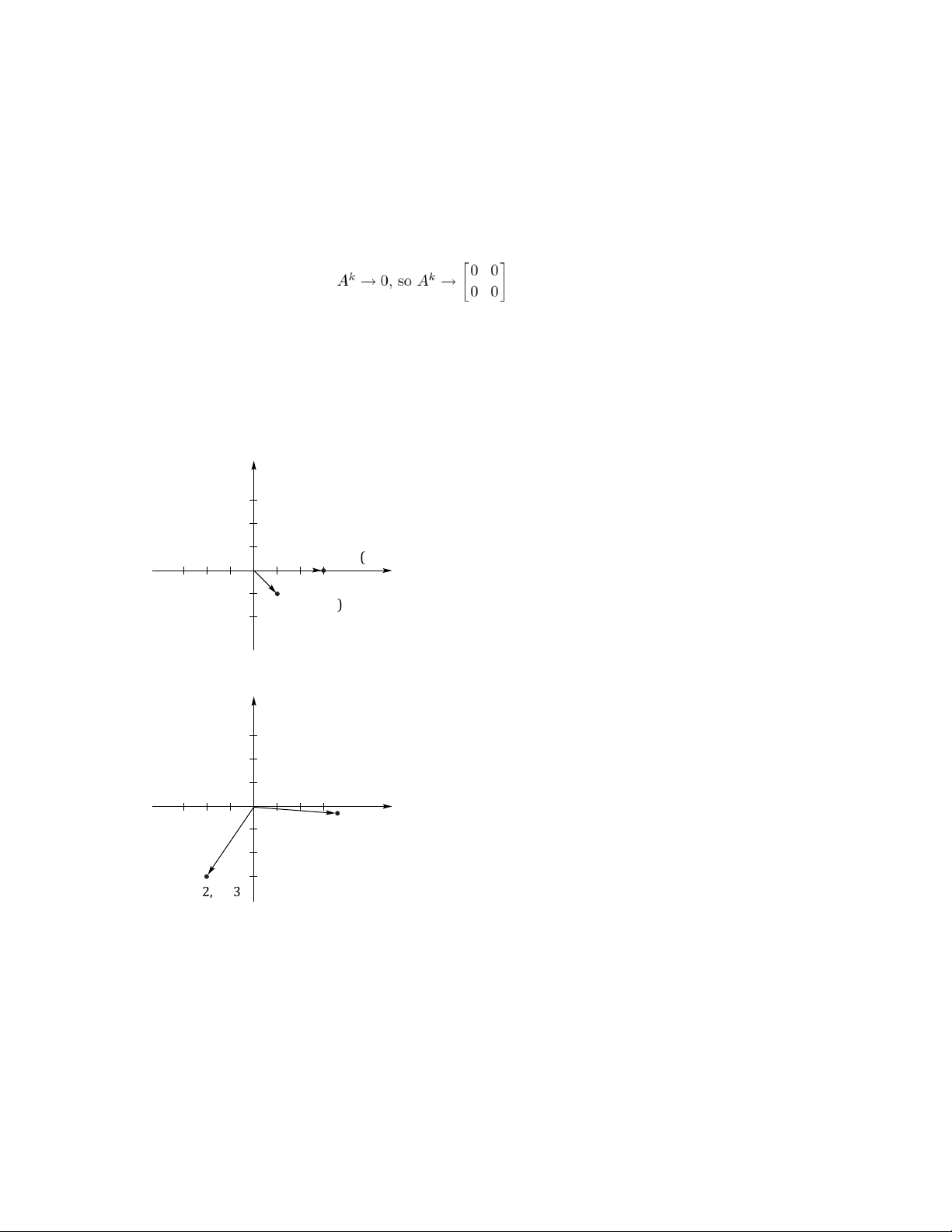
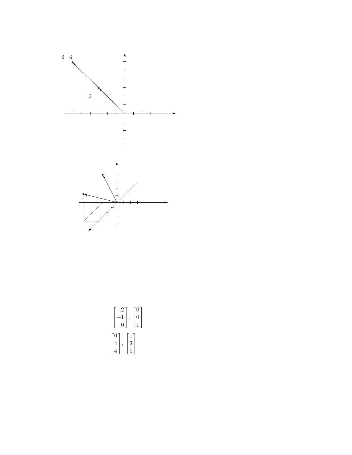
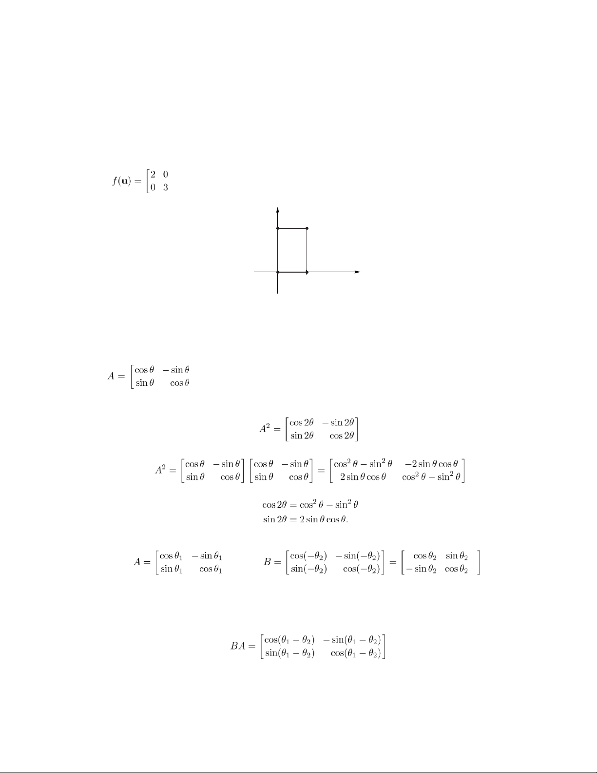
(b) As k → ∞, some of the entries in Ak do not approach 0, so Ak does not approach any matrix. Section 1.6, p. 62 2. y 3 1 f ( ) (3 , 0) u = x − 3 − 1 O 1 3 (1 , − ) 2 u = 4. y 3 1 O x − 2 − 1 1 2
f ( u ) = (6.19 , − 0.23) u = ( 2, −− 3) lOMoAR cPSD| 35974769 20 Chapter 1 Section 1.6 6. y ( 6
− , 6) f ( u ) = − 2u 6 4 u = ( 3 − , 3) 2 x − 6 − 4 − 2 O 1 8. z
u = (0 , − 2 , 4)
f ( u ) = (4 , − 2 , 4) 1 y 1 O 1 x 10 .No. 12. Yes. 14. No. 16.
(a) Reflection about the line y = x.
(b) Reflection about the line y = −x. 18. (a) Possible answers: . (b) Possible answers: .
20. (a) f(u + v) = A(u + v) = Au + Av = f(u) + f(v).
(b) f(cu) = A(cu) = c(Au) = cf(u).
(c) f(cu + dv) = A(cu + dv) = A(cu) + A(cv) = c(Au) + d(Av) = cf(u) + df(v). lOMoAR cPSD| 35974769 21
21. For any real numbers c and d, we have f(cu + dv) = A(cu + dv) = A(cu) + A(dv) = c(Au) + d(Av) = cf(u) +
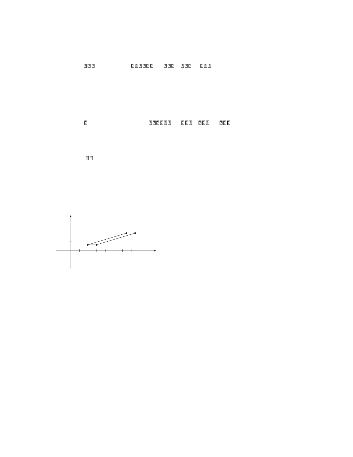
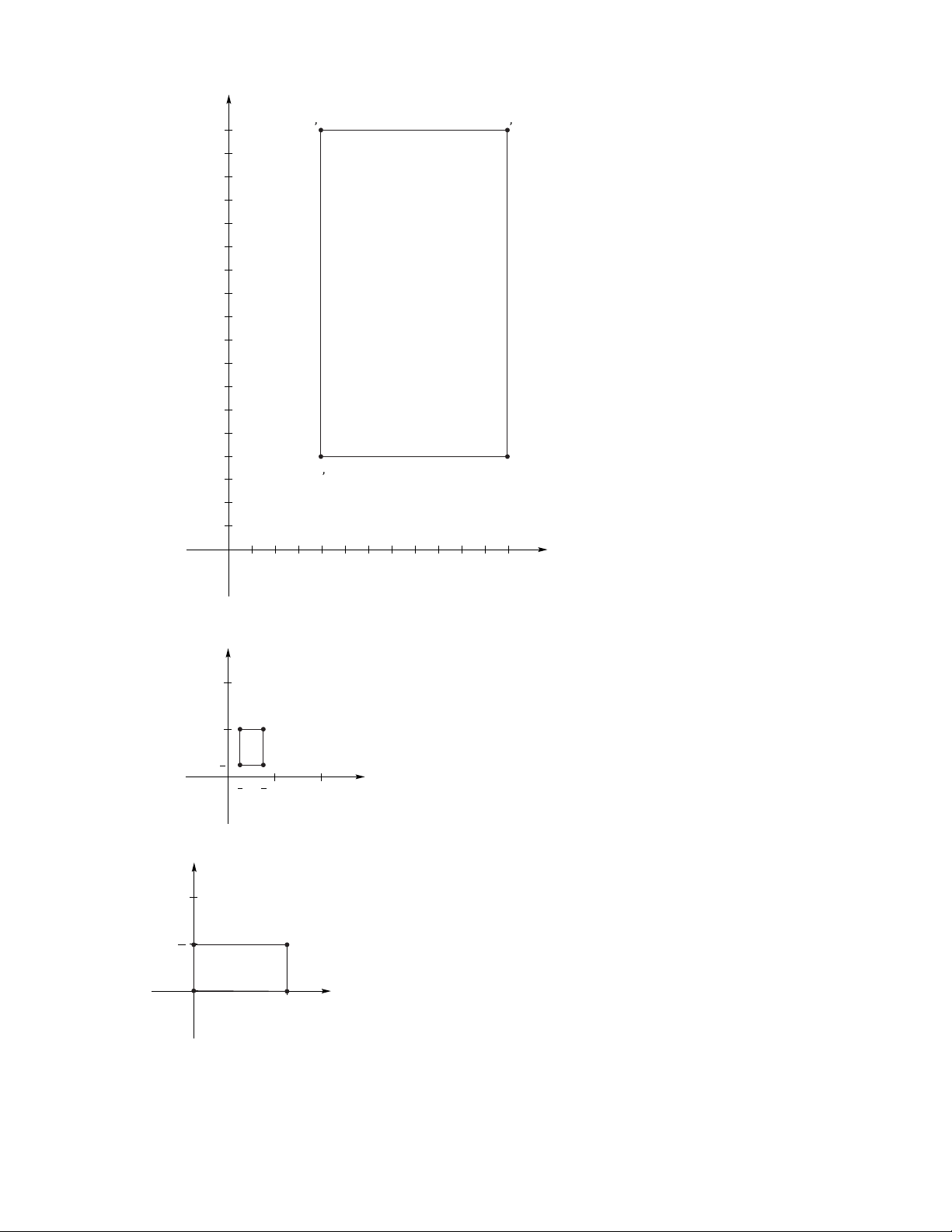
df(v) = c0 + d0 = 0 + 0 = 0. 22. (a) O(u) = 0 ···... 00 u...1 = 0... = 0. 0 ··· un 0 (b) I(u) = 1 0 ···... 0 u...1 = u...1 = u. 0 0 ··· 1 un un Section 1.7, p. 70 2. y 4 2 x O 246810121416 4. ( a ) y lOMoAR cPSD| 35974769 22 Chapter 1 , (4 16) ( , 12 16) 16 12 8 4 , (4 4) (12 , 4) 3 1 x O 1 3 4 8 12 Section 1.7 ( b ) y 2 1 1 4 x 1 O 4 3 4 1 2 6. y 1 1 2 x O 1
8.(1 , − 2) , ( − 3 , 6),(11 , − 10). lOMoAR cPSD| 35974769 23 10. We find that
(f1 ◦ f2)(e1) = e2 (f2 ◦
f1)(e1) = −e2.
Therefore f1 ◦ f2 =& f2 ◦ f1. 12. Here
(u. The new vertices are (0,0), (2,0), (2,3), and (0,3). y (2 , 3) 3 x O 2 14.
(a) Possible answer: First perform f1 (45◦ counterclockwise rotation), then f2.
(b) Possible answer: First perform f3, then f2. 16. Let
(. Then A represents a rotation through the angle θ. Hence A2 represents a
rotation through the angle 2θ, so . Since , we conclude that 17. Let ( and .
Then A and B represent rotations through the angles θ1 and −θ2, respectively. Hence BA represents a
rotation through the angle θ1 − θ2. Then . Since lOMoAR cPSD| 35974769 24 Chapter 1 , we conclude that . Section 1.8, p. 79
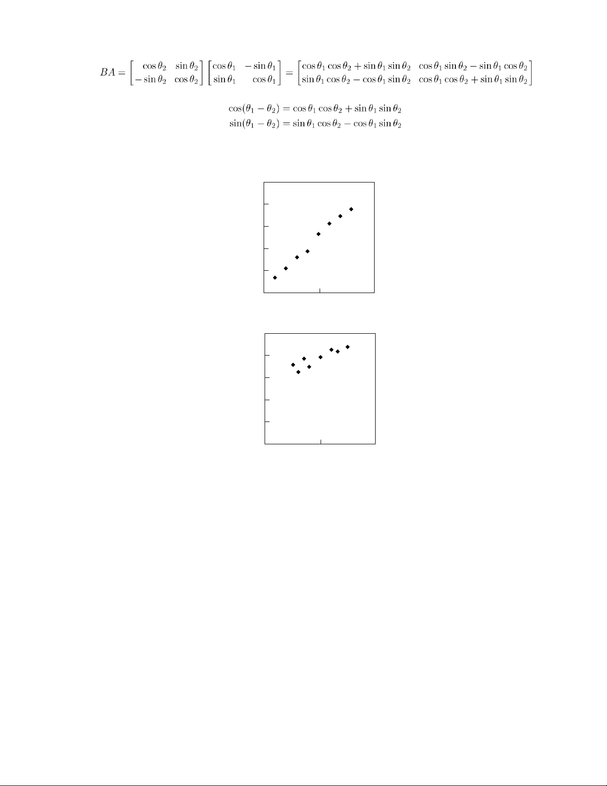
2. Correlation coefficient = 0.9981. Quite highly correlated. 10 8 6 4 2 0 0 5 10
4. Correlation coefficient = 0.8774. Moderately positively correlated. 100 80 60 40 20 0 0 50 100 lOMoAR cPSD| 35974769 Supplementary Exercises 25
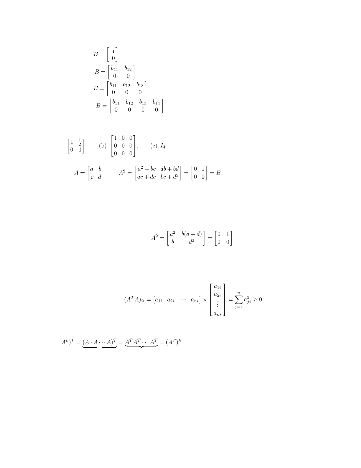
Supplementary Exercises for Chapter 2. (a) k = 1 1, p. 80 . b k = 2 . k = 3 . k = 4 .
(b) The answers are not unique. The only requirement is that row 2 of B have all zero entries. 4. (a) . (d) Let (. Then implies
b(a + d) = 1 c(a + d) = 0.
It follows that a + d = 0& and c = 0. Thus .
Hence, a = d = 0, which is a contradiction; thus, B has no square root.
5. (a) (ATA)ii = (rowiAT) × (coliA) = (coliA)T × (coliA) (b) From part (a) .
(c) ATA = On if and only if (ATA)ii = 0 for i = 1, ..., n. But this is possible if and only if aij = 0 for i = 1, ..., n and
j = 1, ..., n 6. ( . k times67 k times
7. Let A be a symmetric upper (lower) triangular matrix. Then aij = aji and aij = 0 for j > i (j < i). Thus, aij = 0
whenever i =& j, so A is diagonal.
8. If A is skew symmetric then AT = −A. Note that xTAx is a scalar, thus (xTAx)T = xTAx. That is, lOMoAR cPSD| 35974769 26 Chapter 1
xTAx = (xTAx)T = xTATx = −(xTAx). The only
scalar equal to its negative is zero. Hence xTAx = 0 for all x.
9. We are asked to prove an “if and only if” statement. Hence two things must be proved.
(a) If A is nonsingular, then aii = 0& for i = 1, ..., n.
Proof: If A is nonsingular then A is row equivalent to In. Since A is upper triangular, this can occur
only if we can multiply row i by 1/aii for each i. Hence aii = 0& for i = 1, ..., n. (Other row operations
will then be needed to get In.)
(b) If aii &= 0 for i = 1, ..., n then A is nonsingular.
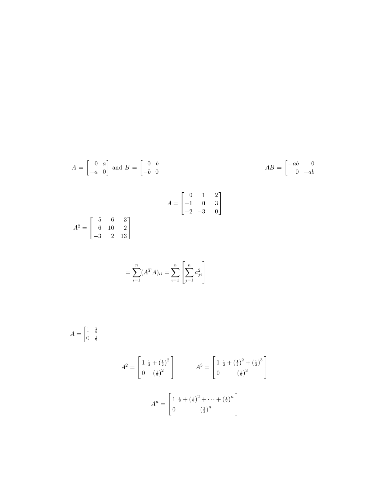
Proof: Just reverse the steps given above in part (a). 10. Let
(. Then A and B are skew symmetric and (
which is diagonal. The result is not true for n > 2. For example, let . Then .
11. Using the definition of trace and Exercise 5(a), we find that
Tr(ATA) = sum of the diagonal entries of ATA (definition of trace) (Exercise 5(a))
= sum of the squares of all entries of A
Thus the only way Tr(ATA) = 0 is if aij = 0 for i = 1, ..., n and j = 1, ..., n. That is, if A = O.
12. When AB = BA. 13. Let (. Then and .
Following the pattern for the elements we have .
A formal proof by induction can be given. lOMoAR cPSD| 35974769 Supplementary Exercises 27
14. Bk = PAkP−1.
15. Since A is skew symmetric, AT = −A. Therefore,
A[−(A−1)T] = −A(A−1)T = AT(A−1)T = (A−1A)T = IT = I
and similarly, [−(A−1)T]A = I. Hence −(A−1)T = A−1, so (A−1)T = −A−1, and therefore A−1 is skew symmetric.
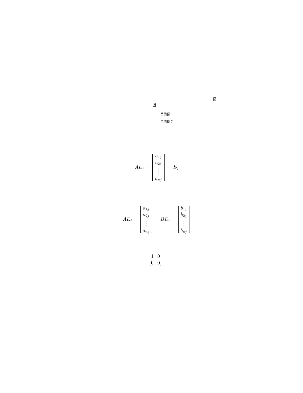
16. If Ax = 0 for all n×1 matrices x, then AEj = 0, j = 1,2,. .,n where Ej = column j of In. But then a1j AEj = ...j = 0. a2 anj
Hence column j of A = 0 for each j and it follows that A = O.
17. If Ax = x for all n × 1 matrices X, then AEj = Ej, where Ej is column j of In. Since
it follows that aij = 1 if i = j and 0 otherwise. Hence A = In.
18. If Ax = Bx for all n×1 matrices x, then AEj = BEj, j = 1,2,. .,n where Ej = column j of In. But then .
Hence column j of A = column j of B for each j and it follows that A = B.
19. (a) In2 = In and O2 = O 0 0 '( b) One such matrix is( and another is. 0 1
(c) If A2 = A and A−1 exists, then A−1(A2) = A−1A which simplifies to give A = In.
20. We have A2 = A and B2 = B.
(a) (AB)2 = ABAB = A(BA)B = A(AB)B (since AB = BA)
= A2B2 = AB
(since A and B are idempotent)
(b) (AT)2 = ATAT = (AA)T
(by the properties of the transpose)
= (A2)T = AT
(since A is idempotent)
(c) If Aand B are n × n and idempotent, then A + B need not be idempotent. For example, let lOMoAR cPSD| 35974769 28 Chapter 1 1 1 0 0 A =( and B = '
(. Both A and B are idempotent and(. However, ' 0 0 1 1 2 2
'C 2 =( =& C. 2 2
(d) k = 0and k = 1.
21. (a) We prove this statement using induction. The result is true for n = 1. Assume it is true for n = k so
that Ak = A. Then
Ak+1 = AAk = AA = A2 = A.
Thus the result is true for n = k + 1. It follows by induction that An = A for all integers n ≥ 1. (b) (In −
A)2 = In2 − 2A + A2 = In − 2A + A = In − A.
22. (a) If A were nonsingular then products of A with itself must also be nonsingular, but Ak is singular since
it is the zero matrix. Thus A must be singular. (b) A3 = O.
(c) k = 1 A = O; In − A = In; (In − A)−1A = In k = 2 A2 = O; (In − A)(In + A) = In − A2 = In; (In − A)−1 = In + A
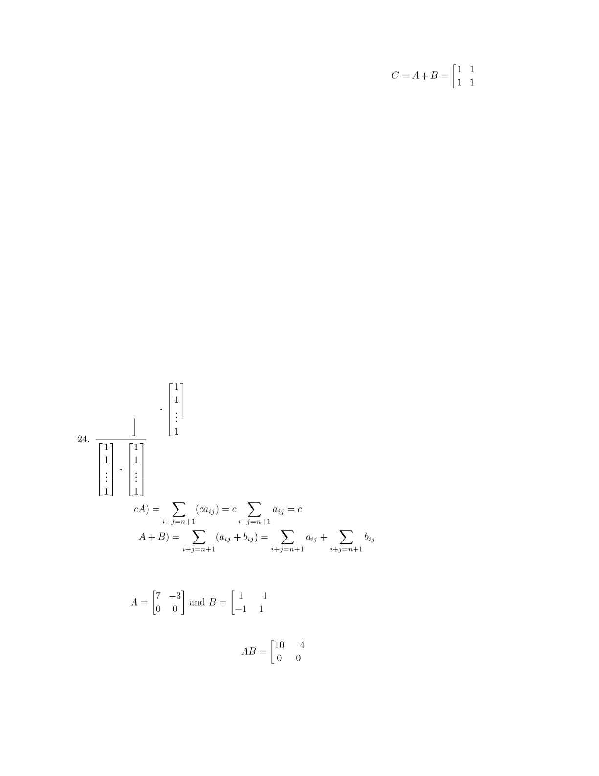
k = 3 A3 = O; (In − A)(In + A + A2) = In − A3 = In; (In − A)−1 = In + A + A2 etc. v 25. (a) Mcd( Mcd(A) (b) Mcd(
= Mcd(A) + Mcd(B)
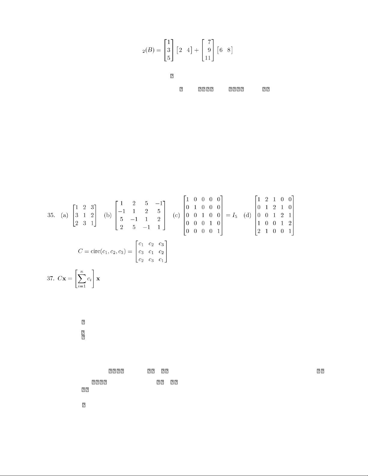
(c) Mcd(AT) = (AT)1n + (AT)2n−1 + ··· + (AT)n1 = an1 + an−12 + ··· + a1n = Mcd(A) (d) Let (. Then ( with Mcd(AB) = 4 lOMoAR cPSD| 35974769 Supplementary Exercises 29 and (
with Mcd(BA) = −10. 1 2 0 0 26. (a) 3 4 0 0 . 0 0 1 0 0 0 2 3 (b) Solve ( obtaining y ( and z (. Then the solution
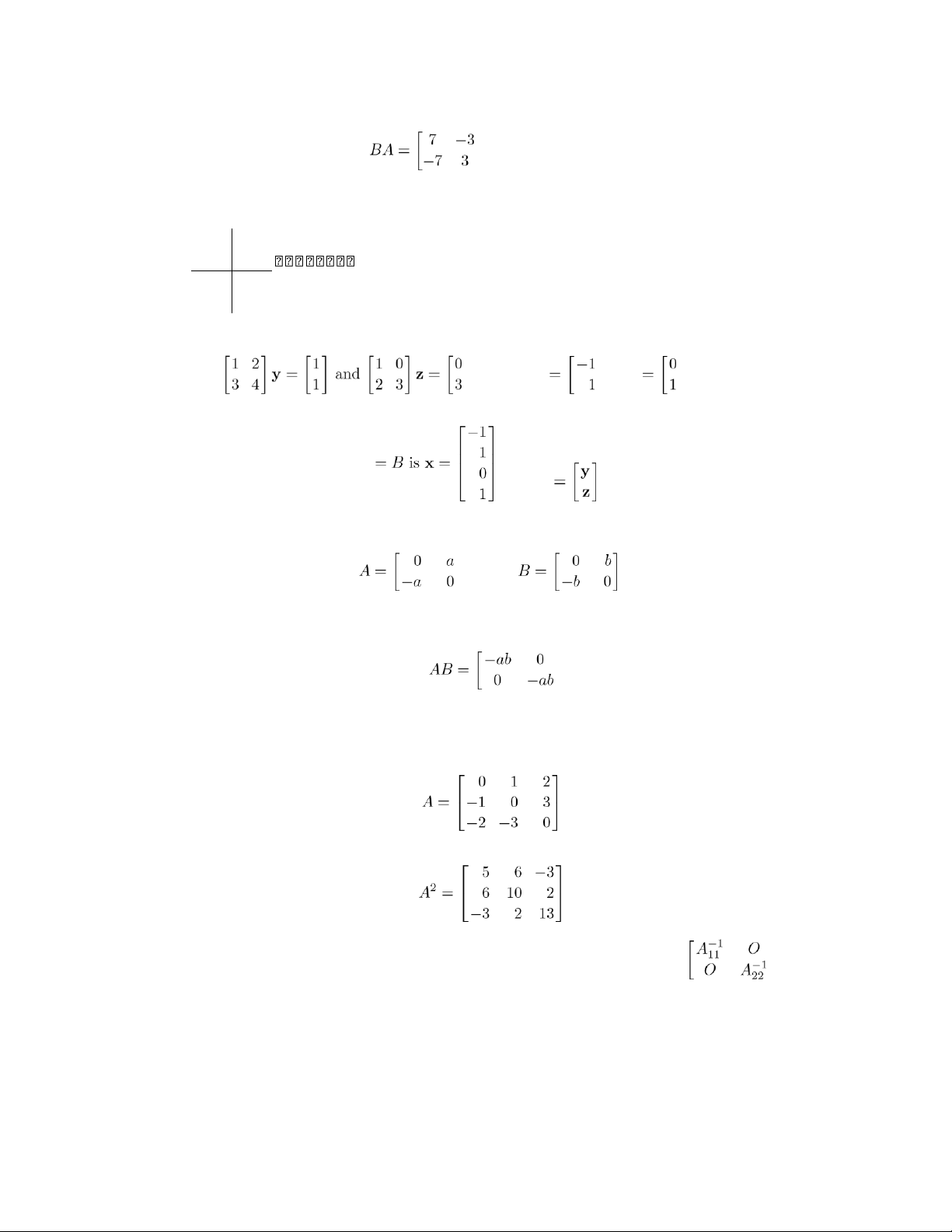
to the given linear system Ax where x . 27. Let ( and .
Then A and B are skew symmetric and (
which is diagonal. The result is not true for n > 2. For example, let . Then .
28. Consider the linear system Ax = 0. If A11 and A22 are nonsingular, then the matrix (
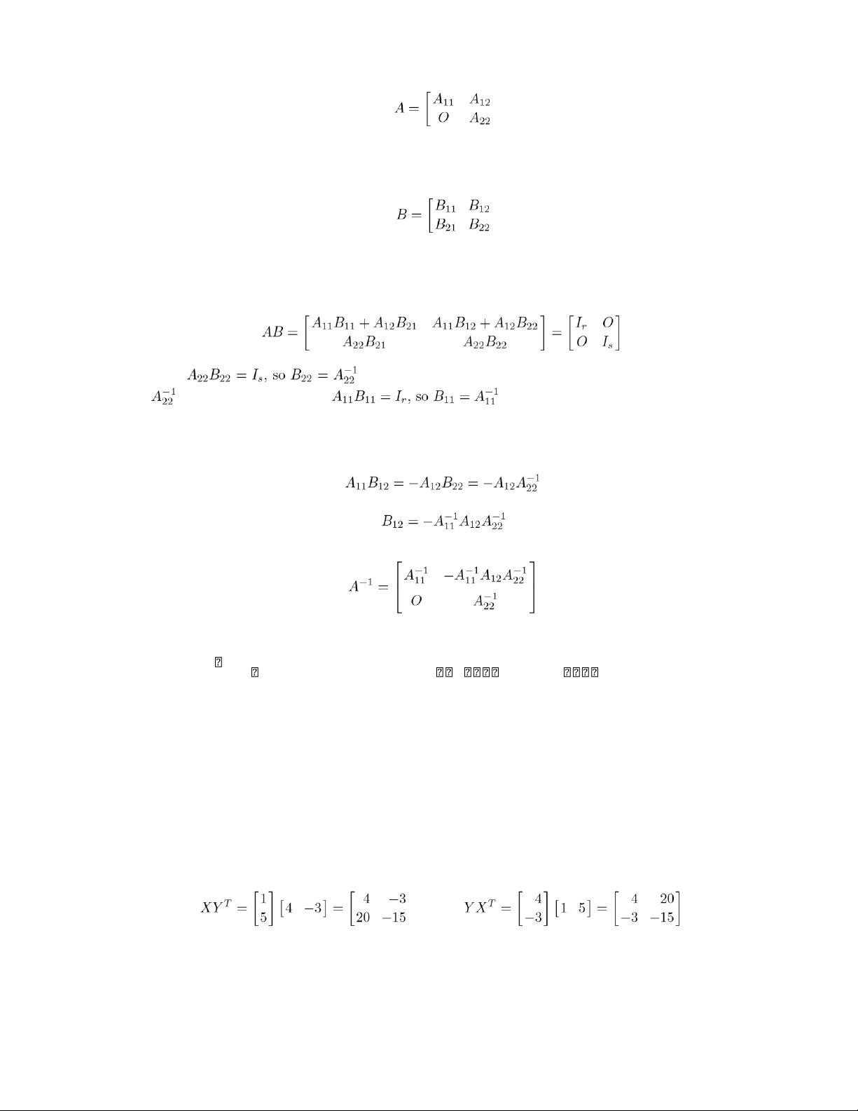
is the inverse of A (verify by block multiplying). Thus A is nonsingular. 29. Let lOMoAR cPSD| 35974769 30 Chapter 1 (
where A11 is r × r and A22 is s × s. Let (
where B11 is r × r and B22 is s × s. Then . We have
. We also have A22B21 = O, and multiplying both sides of this equation by
, we find that B21 = O. Thus . Next, since
A11B12 + A12B22 = O then Hence, .
Since we have solved for B11, B12, B21, and B22, we conclude that A is nonsingular. Moreover, . 4 5 6 −1 0 3 5
30. (a) XY T =8 10 12 . (b) XY T = −2 0 6 10 . 12 15 18 −1 0 3 5 −2 0 6 10 T
31. Let X = 01 51 and Y = 04 −31T. Then ( and .
It follows that XY T is not necessarily the same as Y XT.
32. Tr(XY T) = x1y1 + x2y2 + ··· + xnyn
(See Exercise 27) = XTY . lOMoAR cPSD| 35974769 Supplementary Exercises 31
33. col1(A) × row1(B) + col2(A) × row 2 4 42 56 44 60 =6 12 + 54 72 = 60 84 = AB. 10 20 66 88 76 108
34. (a) HT = (In − 2WWT)T = InT − 2(WWT)T = In − 2(WT)TWT = In − 2WWT = H. (b) HHT = HH = (In − 2WWT)(In − 2WWT)
= In − 4WWT + 4WWTWWT
= In − 4WWT + 4W(WTW)WT
= In − 4WWT + 4W(In)WT = In Thus, HT = H−1. 36. We have
. Thus C is symmetric if and only if c2 = c3. . 38. We proceed directly. c1 c3 c2 c1 c2 c3
c21 + c23 + c22
c1c2 + c3c1 + c2c3 c1c3 +
c3c2 + c2c1 c3 c2 c1 c2 c3 c1
c3c1 + c2c3 + c1c2 c3c2 + c2c1 +
c1c3 c32 + c22 + c21 CTC =c2 c1 c3 c3 c1 c2 =
c2c1 + c1c3 + c3c2
c22 + c21 + c23
c2c3 + c1c2 + c3c1
CCT =c3 c1 c2 c2 c1 c3 =
c3c1 + c1c2 + c2c3
c32 + c21 + c22
c3c2 + c1c3 + c2c1 . c1 c2 c3 c1 c3 c2
c21 + c22 + c32
c1c3 + c2c1 + c3c2 c1c2 +
c2c3 + c3c1 c2 c3 c1 c3 c2 c1
c2c1 + c3c2 + c1c3
c2c3 + c3c1 + c1c2
c22 + c23 + c12 lOMoAR cPSD| 35974769 32 Chapter 1
It follows that CTC = CCT.
Chapter Review for Chapter 1, p. 83 True or False 1. False.
2. False. 3. True. 4. True. 5. True. 6. True. 7. True. 8. True. 9. True. 10. True. lOMoAR cPSD| 35974769 33 Chapter Review Quiz ' 1. x =(. 2 −4 2. r = 0. 3. a = b = 4. 4. (a) a = 2.
(b) b = 10, c = any real number. 5.
(, where r is any real number. lOMoAR cPSD| 35974769 Chapter 2 Solving Linear Systems Section 2.1, p. 94
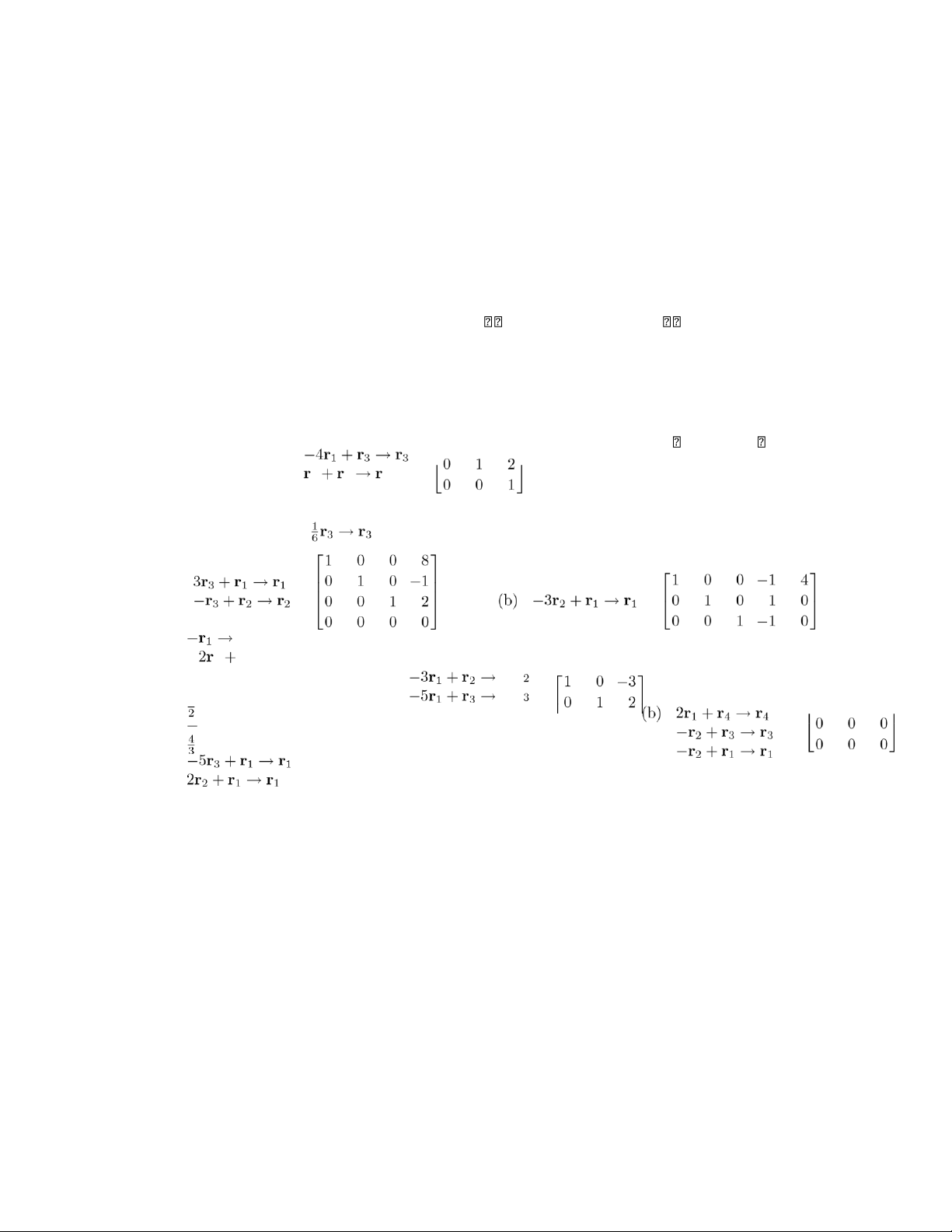
2. (a) Possible answer:−3−rr141rr+11 →r2 r→→1 r2r3 10 −11 14 01 −31 + r3 → 2 2 + r3 r3 0 0 0 0 0
2r1 + r2 → r2 1 1 −4 (b) Possible answer: 2 3 3 4. (a) r1 −2r11 + rr2 r 3 →→ rr23 r 6.
(a) −1r32r→→rr22r→3 r2 I3 3 r3 + 8. (a) REF (b) RREF (c) N
9. Consider the columns of A which contain leading entries of nonzero rows of A. If this set of columns is
the entire set of n columns, then A = In. Otherwise there are fewer than n leading entries, and hence
fewer than n nonzero rows of A.
10. (a) A is row equivalent to itself: the sequence of operations is the empty sequence.
(b) Each elementary row operation of types I, II or III has a corresponding inverse operation of thesame
type which “undoes” the effect of the original operation. For example, the inverse of the operation
“add d times row r of A to row s of A” is “subtract d times row r of A from row s of A.” Since B is
assumed row equivalent to A, there is a sequence of elementary row operations which gets from A
to B. Take those operations in the reverse order, and for each operation do its inverse, and that takes
B to A. Thus A is row equivalent to B. lOMoAR cPSD| 35974769
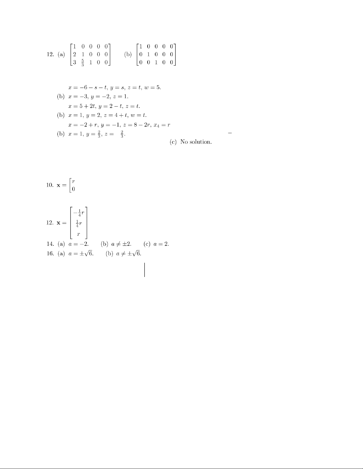
(c) Follow the operations which take A to B with those which take B to C. lOMoAR cPSD| 35974769 36 Chapter 2 Section 2.2, p. 113 2. (a) 4. (a) 6. (a)
, where r is any real number.
8. (a) x = 1 − r, y = 2, z = 1, x4 = r,
where r is any real number.
(b) x = 1 − r, y = 2 + r, z = −1 + r, x4 = r, where r is any real number. (, where r &= 0. , where r &= 0. ' a b0 c d0
18. The augmented matrix is(. If we reduce this matrix to reduced row echelon form, we see
that the linear system has only the trivial solution if and only if A is row equivalent to I2. Now show
that this occurs if and only ifis row equivalent to a matrix that has a row or column consisting entirely of
zeros, so thatad − bc &= 0. If ad − bcI2&= 0. Ifthen at least one ofad − bc = 0, then by case considerations
wea or c is = 0& , and it is a routine matter to show that A is row equivalent to find that A
A is not row equivalent to I2.
adAlternate proof: Ifbc = 0, then adad=−bcbc. If= 0& ad, then= 0 then eitherA is nonsingular, so the only
solution is the trivial one. Ifa or d = 0, say a = 0. Then bc = 0, and either b or c−= 0. In any of these cases lOMoAR cPSD| 35974769 37
we get a nontrivial solution. If ad &= 0, then ac = db, and the second equation is a multiple of the first one
so we again have a nontrivial solution.
19. This had to be shown in the first proof of Exercise 18 above. If the alternate proof of Exercise 18 wasgiven,
then Exercise 19 follows from the former by noting that the homogeneous system Ax = 0 has only the
trivial solution if and only if A is row equivalent to I2 and this occurs if and only if ad−bc &= 0.
, where t is any number.
22. −a + b + c = 0.
24. (a) Change “row” to “column.”
(b) Proceed as in the proof of Theorem 2.1, changing “row” to “column.” Section 2.2
25. Using Exercise 24(b) we can assume that every m × n matrix A is column equivalent to a matrix in column
echelon form. That is, A is column equivalent to a matrix B that satisfies the following:
(a) All columns consisting entirely of zeros, if any, are at the right side of the matrix.
(b) The first nonzero entry in each column that is not all zeros is a 1, called the leading entry of thecolumn.
(c) If the columns j and j + 1 are two successive columns that are not all zeros, then the leading entry of
column j + 1 is below the leading entry of column j.
We start with matrix B and show that it is possible to find a matrix C that is column equivalent to B that satisfies
(d) If a row contains a leading entry of some column then all other entries in that row are zero.
If column j of B contains a nonzero element, then its first (counting top to bottom) nonzero element is a
1. Suppose the 1 appears in row rj. We can perform column operations of the form acj + ck for each of the
nonzero columns ck of B such that the resulting matrix has row rj with a 1 in the (rj,j) entry and zeros
everywhere else. This can be done for each column that contains a nonzero entry hence we can produce
a matrix C satisfying (d). It follows that C is the unique matrix in reduced column echelon form and column
equivalent to the original matrix A.
26. −3a − b + c = 0.
28. Apply Exercise 18 to the linear system given here. The coefficient matrix is .
Hence from Exercise 18, we have a nontrivial solution if and only if (a − r)(b − r) − cd = 0.
29. (a) A(xp + xh) = Axp + Axh = b + 0 = b. lOMoAR cPSD| 35974769 38
(b) Let xp be a particular solution to Ax = b and let x be any solution to Ax = b. Let xh = x−xp. Then x = xp
+ xh = xp + (x − xp) and Axh = A(x − xp) = Ax − Axp = b − b = 0. Thus xh is in fact a solution to Ax = 0.
30. (a) 3x2 + 2 (b) 2x2 − x − 1 = 0
(b) x = 5, y = −7
36. r = 5, r2 = 5.
37. The GPS receiver is located at the tangent point where the two circles intersect. 38. 4Fe + 3O2 → 2Fe2O3 . 42. No solution. Chapter 1 Section 2.3, p. 124
1. The elementary matrix E which results from In by a type I interchange of the ith and jth row differs from
In by having 1’s in the (i,j) and (j,i) positions and 0’s in the (i,i) and (j,j) positions. For that E, EA has as its
ith row the jth row of A and for its jth row the ith row of A.
The elementary matrix E which results from In by a type II operation differs from In by having c = 0& in
the (i,i) position. Then EA has as its ith row c times the ith row of A.
The elementary matrix E which results from In by a type III operation differs from In by having c in the (j,i)
position. Then EA has as jth row the sum of the jth row of A and c times the ith row of A. 2. (a) .
4. (a) Add 2 times row 1 to row 3: (b) Add 2 times row 1 to row 3: .
Therefore B is the inverse of A. lOMoAR cPSD| 35974769 39
6. If E1 is an elementary matrix of type I then E1−1 = E1. Let E2 be obtained from In by multiplying the ith row
of In by c = 0& . Let be obtained from In by multiplying the ith row of In by 1c. Then
be obtained from In by adding c times the ith row of In to the jth row of In. Let
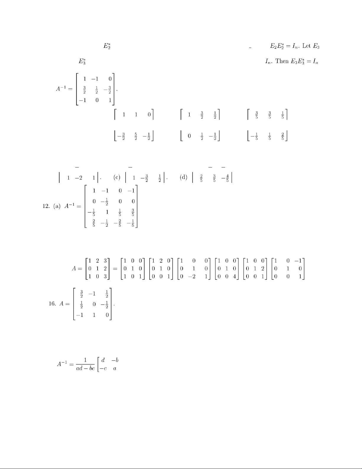
be obtained from In by adding −c times the ith row of In to the jth row of . 8. 10. (a) Singular. (b) . . (b) Singular. Section 2.3
14. A is row equivalent to I3; a possible answer is . 18. (b) and (c).
20. For a = −1 or a = 3.
21. This follows directly from Exercise 19 of Section 2.1 and Corollary 2.2. To show that ( we proceed as follows: lOMoAR cPSD| 35974769 40 .
23. The matrices A and B are row equivalent if and only if B = EkEk−1 ···E2E1A. Let P = EkEk−1 ···E2E1.
24. If A and B are row equivalent then B = PA, where P is nonsingular, and A = P−1B (Exercise 23). If A is
nonsingular then B is nonsingular, and conversely.
25. Suppose B is singular. Then by Theorem 2.9 there exists x =& 0 such that Bx = 0. Then (AB)x = A0 = 0,
which means that the homogeneous system (AB)x = 0 has a nontrivial solution. Theorem 2.9 implies that
AB is singular, a contradiction. Hence, B is nonsingular. Since A = (AB)B−1 is a product of nonsingular
matrices, it follows that A is nonsingular.
Alternate Proof: If AB is nonsingular it follows that AB is row equivalent to In, so P(AB) = In. Since P is
nonsingular, P = EkEk−1 ···E2E1. Then (PA)B = In or (EkEk−1 ···E2E1A)B = In. Letting EA ···
k=EkP−−11 B−E12, soE1AA=is nonsingular.C, we have CB = In, which implies that B is nonsingular. Since PAB = In,
26. The matrix A is row equivalent to O if and only if A = PO = O where P is nonsingular.
27. The matrix A is row equivalent to B if and only if B = PA, where P is a nonsingular matrix. Now BT = ATPT,
so A is row equivalent to B if and only if AT is column equivalent to BT.
28. If A has a row of zeros, then A cannot be row equivalent to In, and so by Corollary 2.2, A is singular. If the
jth column of A is the zero column, then the homogeneous system Ax = 0 has a nontrivial solution, the
vector x with 1 in the jth entry and zeros elsewhere. By Theorem 2.9, A is singular. 29. (a) No. Let
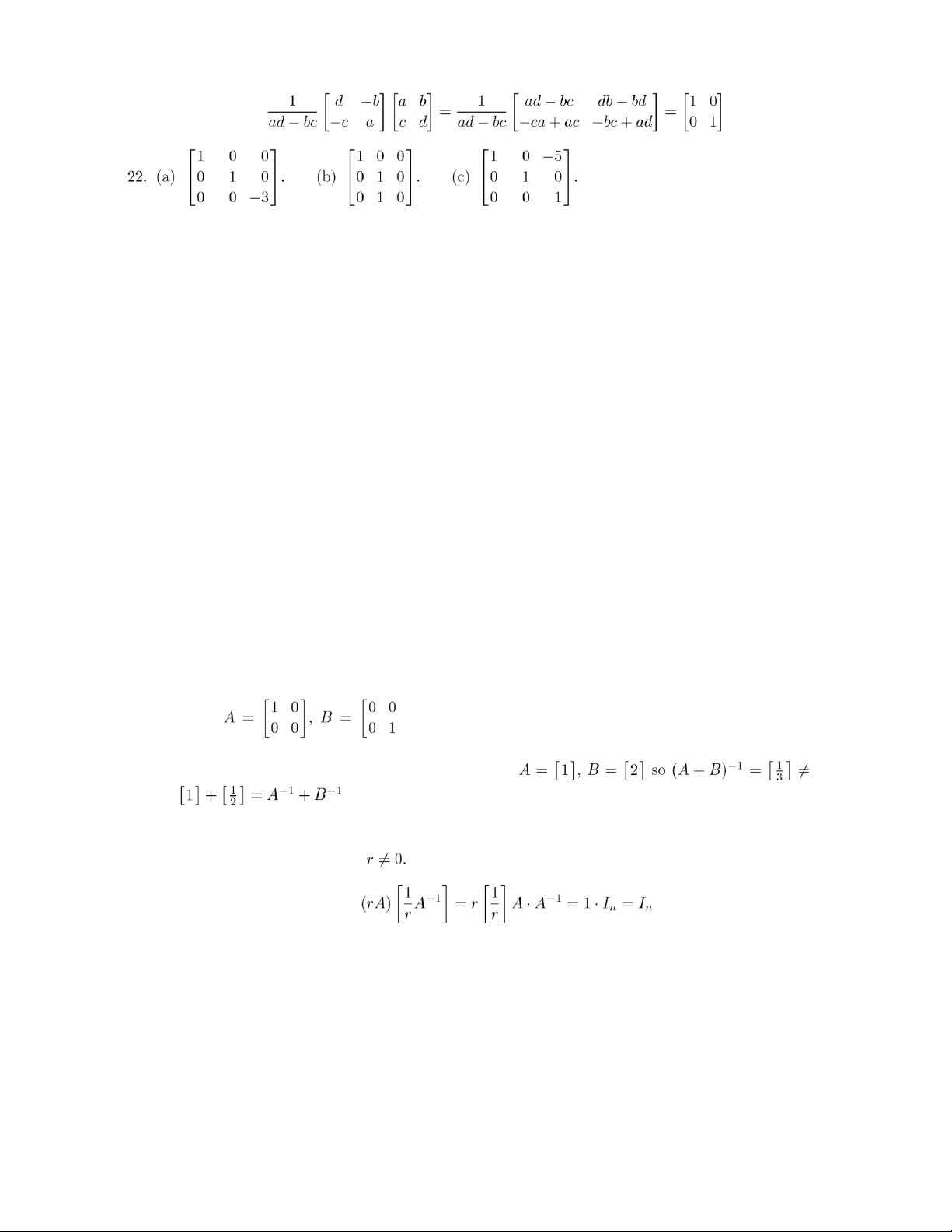
(. Then (A + B)−1 exists but A−1 and B−1 do not. Even
supposing they all exist, equality need not hold. Let . Chapter 1
(b) Yes, for A nonsingular and .
30. Suppose that A is nonsingular. Then Ax = b has the solution x = A−1b for every n × 1 matrix b. Conversely,
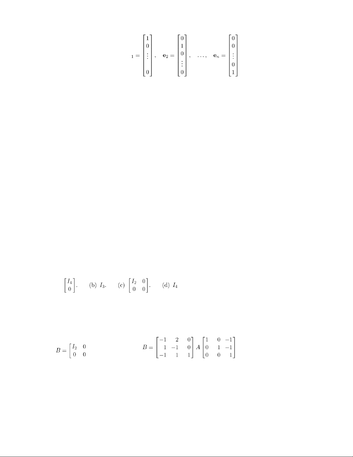
suppose that Ax = b is consistent for every n × 1 matrix b. Letting b be the matrices lOMoAR cPSD| 35974769 41 e ,
we see that we have solutions x1,x2,. .,xn to the linear systems
Ax1 = e1,
Ax2 = e2, . .,
Axn = en. (∗)
Letting C be the matrix whose jth column is xj, we can write the n systems in (∗) as AC = In, since In = 0e1
e2 ··· en1. Hence, A is nonsingular.
31. We consider the case that A is nonsingular and upper triangular. A similar argument can be given for A lower triangular.
By Theorem 2.8, A is a product of elementary matrices which are the inverses of the elementary matrices
that “reduce” A to In. That is,
A = E1−1 ···Ek−1.
The elementary matrix Ei will be upper triangular since it is used to introduce zeros into the upper
triangular part of A in the reduction process. The inverse of Ei is an elementary matrix of the same type
and also an upper triangular matrix. Since the product of upper triangular matrices is upper triangular
and we have A−1 = Ek ···E1 we conclude that A−1 is upper triangular. Section 2.4, p. 129
1. See the answer to Exercise 4, Section 2.1. Where it mentions only row operations, now read “row and column operations”. 2. (a) .
4. Allowable equivalence operations (“elementary row or elementary column operation”) include in
particular elementary row operations.
5. A and B are equivalent if and only if B = Et ···E2E1AF1F2 ···Fs. Let EtEt−1 ···E2E1 = P and F1F2 ···Fs = Q. 6. (; a possible answer is: .
8. Suppose A were nonzero but equivalent to O. Then some ultimate elementary row or column operation
must have transformed a nonzero matrix Ar into the zero matrix O. By considering the types of
elementary operations we see that this is impossible. Section 2.5 lOMoAR cPSD| 35974769 42
9. Replace “row” by “column” and vice versa in the elementary operations which transform A into B. 10. Possible answers are: 4. . 6. . 8. . .
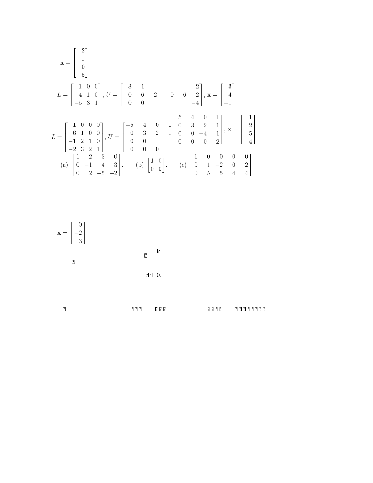
11. If A and B are equivalent then B = PAQ and A = P−1BQ−1. If A is nonsingular then B is nonsingular, and conversely. Section 2.5, p. 136 2. . 1 0 0 0 4 1 0.25 −0.5 −1.5
0.2 1 0 00 0.4 1.2 2.5 4.2
−0.4 0.8 1 00 0 −0.85 2 2.6 2 −1.2 −0.4 1 0 0 0 −2.5 −2 10. L = , U = − , x = .
Supplementary Exercises for Chapter 2, p. 137 2.
(a) a = −4 or a = 2.
(b) The system has a solution for each value of a.
4. c + 2a − 3b = 0.
5. (a) Multiply the jth row of B by k1.
(b) Interchange the ith and jth rows of B. lOMoAR cPSD| 35974769 43
(c) Add −k times the jth row of B to its ith row.
6. (a) If we transform E1 to reduced row echelon form, we obtain In. Hence E1 is row equivalent to In and thus is nonsingular.
(b) If we transform E2 to reduced row echelon form, we obtain In. Hence E2 is row equivalent to In and thus is nonsingular. Chapter 2
(c) If we transform E3 to reduced row echelon form, we obtain In. Hence E3 is row equivalent to In and thus is nonsingular. .
13. For any angle θ, cosθ and sinθ are never simultaneously zero. Thus at least one element in column 1 is not
zero. Assume cosθ = 0. (& If cosθ = 0, then interchange rows 1 and 2 and proceed in a similar manner to
that described below.) To show that the matrix is nonsingular and determine its inverse, we put ' −cosθ
sinθ1 0 ( sinθ cosθ0 1
into reduced row echelon form. Apply row operations
times row 1 and sinθ times row 1 added to row 2 to obtain sin θ 1 1 0 cos θ cos θ . sin 2 θ sin θ 0 + cos θ 1 cos θ cosθ Since sin2 θ
sin2 θ + cos2 θ 1 + cosθ = = , cosθ cosθ cosθ lOMoAR cPSD| 35974769 44
the (2,2)-element is not zero. Applying row operations cosθ times row 2 and : times row 2 added to row 1 we obtain '
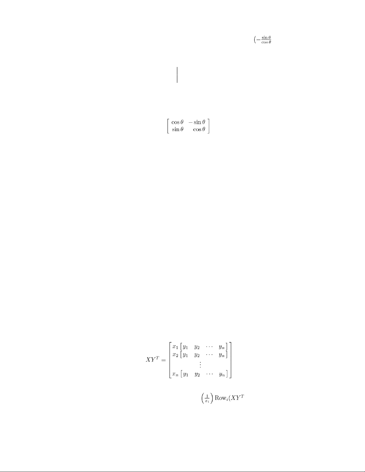
1 0cosθ −sinθ ( . 0 1sinθ cosθ
It follows that the matrix is nonsingular and its inverse is .
14. (a) A(u + v) = Au + Av = 0 + 0 = 0. (b) A(u − v) = Au − Av = 0 − 0 = 0.
(c) A(ru) = r(Au) = r0 = 0.
(d) A(ru + sv) = r(Au) + s(Av) = r0 + s0 = 0.
15. If Au = b and Av = b, then A(u − v) = Au − Av = b − b = 0. Chapter Review
16. Suppose at some point in the process of reducing the augmented matrix to reduced row echelon form
we encounter a row whose first n entries are zero but whose (n+1)st entry is some number c = 0& . The
corresponding linear equation is
0 · x1 + ··· + 0 · xn = c or 0 = c.
This equation has no solution, thus the linear system is inconsistent.
17. Let u be one solution to Ax = b. Since A is singular, the homogeneous system Ax = 0 has a nontrivial
solution u0. Then for any real number r, v = ru0 is also a solution to the homogeneous system. Finally, by
Exercise 29, Sec. 2.2, for each of the infinitely many vectors v, the vector w = u + v is a solution to the
nonhomogeneous system Ax = b.
18. s = 1, t = 1.
20. If any of the diagonal entries of L or U is zero, there will not be a unique solution. 21. The
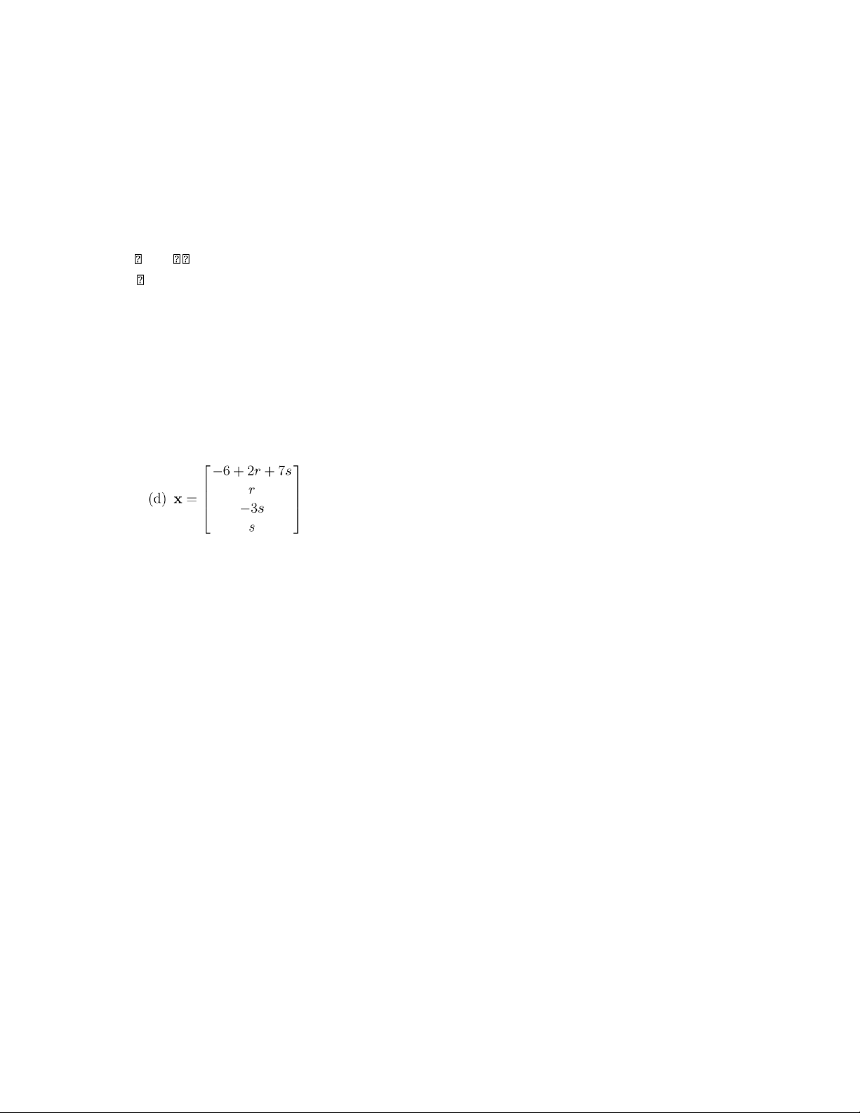
outer product of X and Y can be written in the form .
If either X = O or Y = O, then XY T = O. Thus assume that there is at least one nonzero component in X, say
xi, and at least one nonzero component in Y , say yj. Then
) makes the ith row exactly Y T.
Since all the other rows are multiples of Y T, row operations of the form −xkRi +Rp, for p =& i, can be lOMoAR cPSD| 35974769 45
performed to zero out everything but the ith row. It follows that either XY T is row equivalent to O or to a
matrix with n − 1 zero rows.
Chapter Review for Chapter 2, p. 138 True or False 1. False. 2. True. 3. False. 4. True. 5. True. 6. True. 7. True. 8. True. 9. True. 10. False. Quiz 0 0 0 1 0 2 1.0 1 3 2. (a) No. (b) Infinitely many. (c) No.
, where r and s are any real numbers. 3. k = 6. lOMoAR cPSD| 35974769 Chapter 2 .
7. Possible answers: Diagonal, zero, or symmetric. lOMoAR cPSD| 35974769 Chapter 3 Determinants Section 3.1, p. 145 2. (a) 4. (b) 7. (c) 0. 4. (a) odd. (b) even. (c) even. 6. (a) −. (b) +. (c) +. 8. (a) 7. (b) 2. 10. det ( 12. (a) −24. (b) −36. (c) 180.
14. (a) t2 − 8t − 20. (b) t3 − t.
16. (a) t = 10, t = −2.
(b) t = 0, t = 1, t = −1. Section 3.2, p. 154
2. (a) 4. (b) −24. (c) −30. (d) 72. (e) −120. (f) 0. 4. −2.
6. (a) det(A) = −7, det(B) = 3.
(b) det(A) = −24, det(B) = −30.
8. Yes, since det(AB) = det(A)det(B) and det(BA) = det(B)det(A).
9. Yes, since det(AB) = det(A)det(B) implies that det(A) = 0 or det(B) = 0.
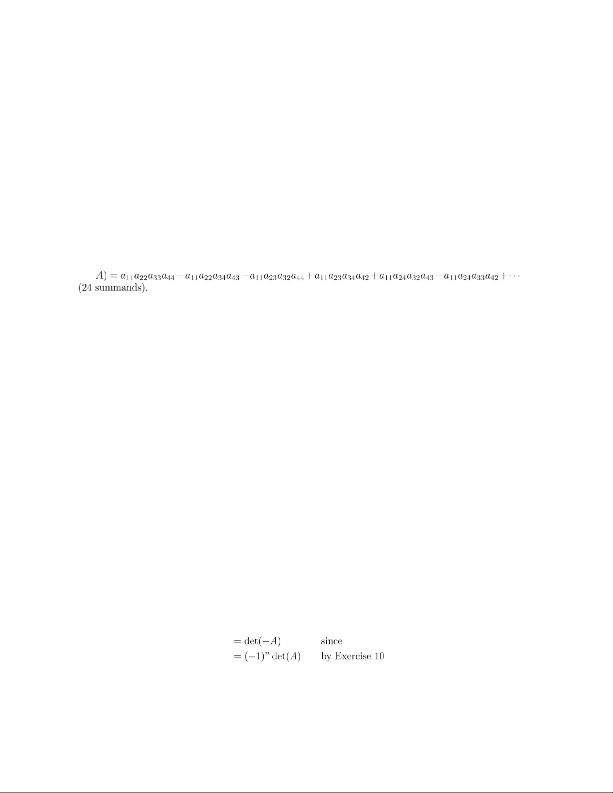
10. det(cA) = 4(±)(ca1j1)(ca2j2)···(−canjn) = cn 4(±)a1j1a2j2 ···anjn = cn det(A).
11. Since A is skew symmetric, AT = A. Therefore
det(A) = det(AT) by Theorem 3.1 since A is skew symmetric by Exercise 10 lOMoAR cPSD| 35974769 48 Chapter 3 = −det(A) since n is odd
The only number equal to its negative is zero, so det(A) = 0.
12. This result follows from the observation that each term in det(A) is a product of n entries of A, each with
its appropriate sign, with exactly one entry from each row and exactly one entry from each column. 13. We have det( .
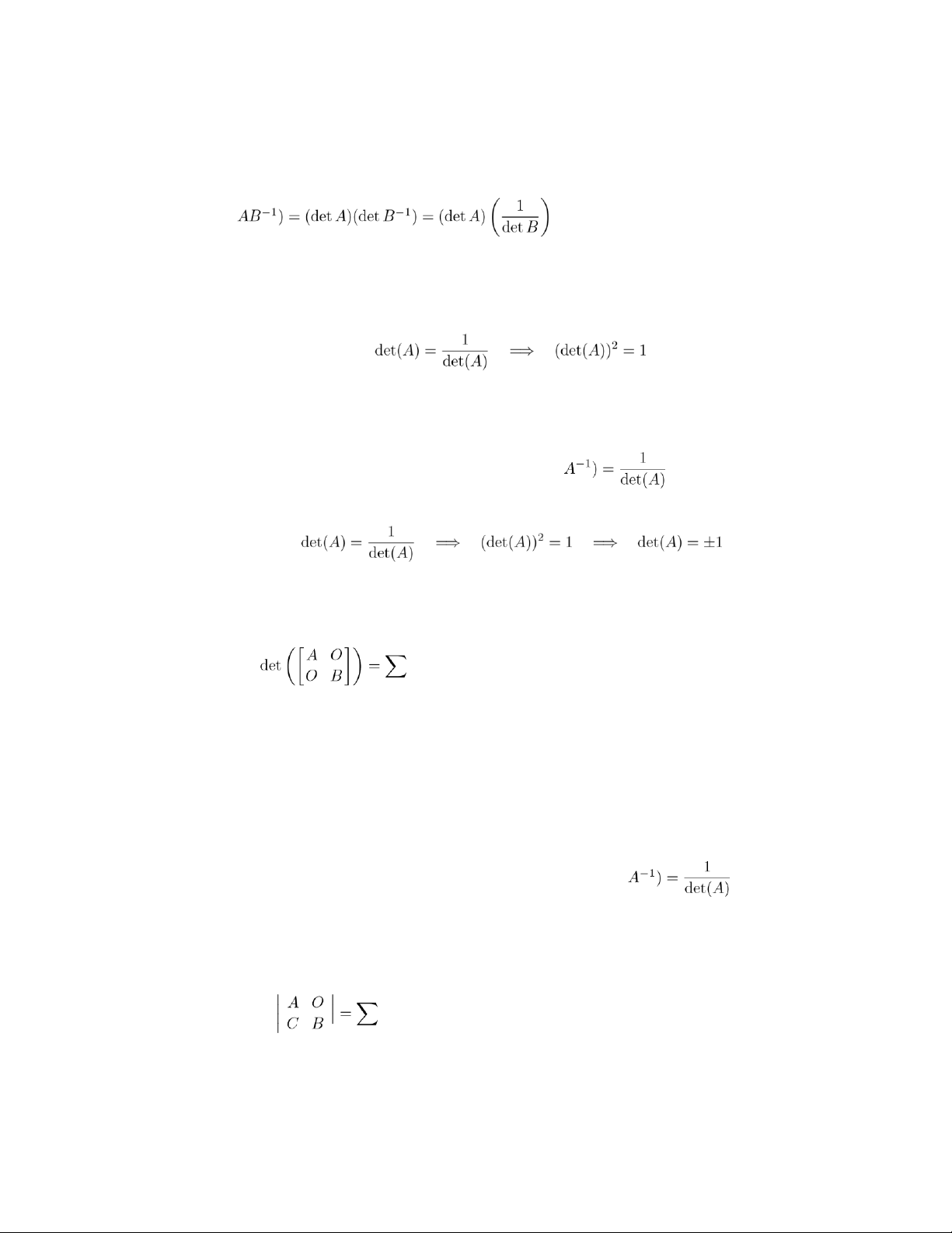
14. If AB = In, then det(AB) = det(A)det(B) = det(In) = 1, so det(A) = 0& and det(B) &= 0. 15. (a) By Corollary
3.3, det(A−1) = 1/det(A). Since A = A−1, we have . Hence det(A) = ±1.
(b) If AT = A−1, then det(AT) = det(A−1). But
det(A) = det(AT) and det( hence we have .
16. From Definition 3.2, the only time we get terms which do not contain a zero factor is when the
termsinvolved come from A and B alone. Each one of the column permutations of terms from A can be
associated with every one of the column permutations of B. Hence by factoring we have
(terms from A for any column permutation)|B|
= |B|)(terms from A for any column permutation)
= (detB)(detA) = (detA)(detB).
17. If A2 = A, then det(A2) = [det(A)]2 = det(A), so det(A) = 1. Alternate solution: If A2 = A and A is nonsingular,
then A−1A2 = A−1A = In, so A = In and det(A) = det(In) = 1.
18. Since AA−1 = In, det(AA−1) = det(In) = 1, so det(A)det(A−1) = 1. Hence, det( .
19. From Definition 3.2, the only time we get terms which do not contain a zero factor is when the
termsinvolved come from A and B alone. Each one of the column permutations of terms from A can be
associated with every one of the column permutations of B. Hence by factoring we have
(terms from A for any column permutations)|B| ? =
|B|)(terms from A for any column permutation) lOMoAR cPSD| 35974769 = |B||A|
20. (a) det(ATBT) = det(AT)det(BT) = det(A)det(BT). (b) det(ATBT) = det(AT)det(BT) = det(AT)det(B).
?????1 a a2????????????1 a a2 ??????
22. ?11 cb cb22 = 00 2cb −− a b22 − aa22
= (b − a)(c2 − a ) − (a cc − a− 2
a2) = (b − a)(c − a)(c + a) − (c − a)(b − a)(b + a) )(b −
= (b − a)(c − a)[(c + a) − (b + a)] = (b − a)(c − a)(c − b). lOMoAR cPSD| 35974769 50 Chapter 3 Section 3.3 24. (a) and (b). 26. (a) t &= 0. (b) t &= ±1.
(c) t &= 0,±1.
28. The system has only the trivial solution.
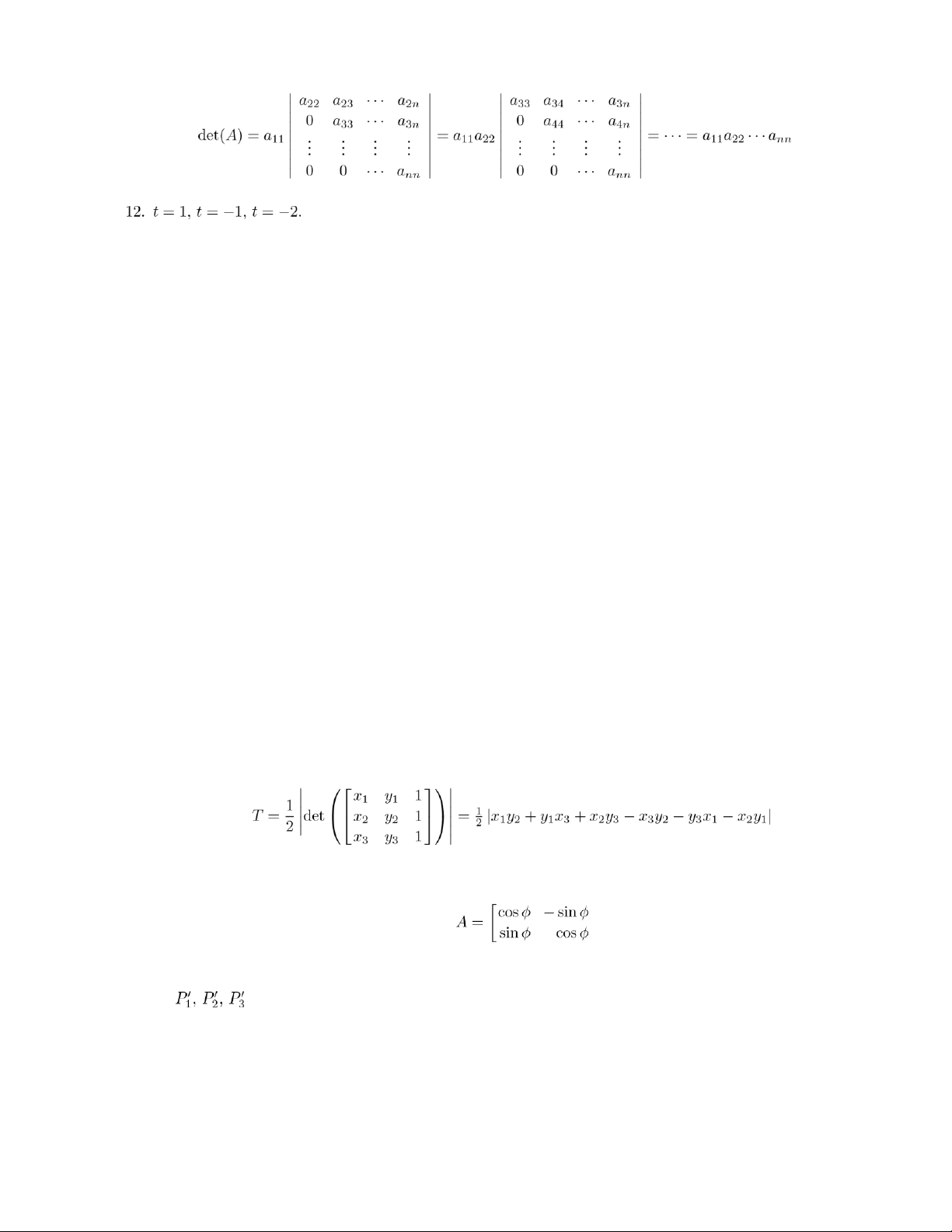
29. Ifi A = 0aij1 is upper triangular, then det(A) = a11a22 ···ann, so det(A) &= 0 if and only if aii &= 0 for ,. .,n.
(b) Only the trivial solution.
31. (a) A matrix having at least one row of zeros. (b) Infinitely many.
32. If A2 = A, then det(A2) = det(A), so [det(A)]2 = det(A). Thus, det(A)(det(A) − 1) = 0. This implies that det(A) = 0 or det(A) = 1.
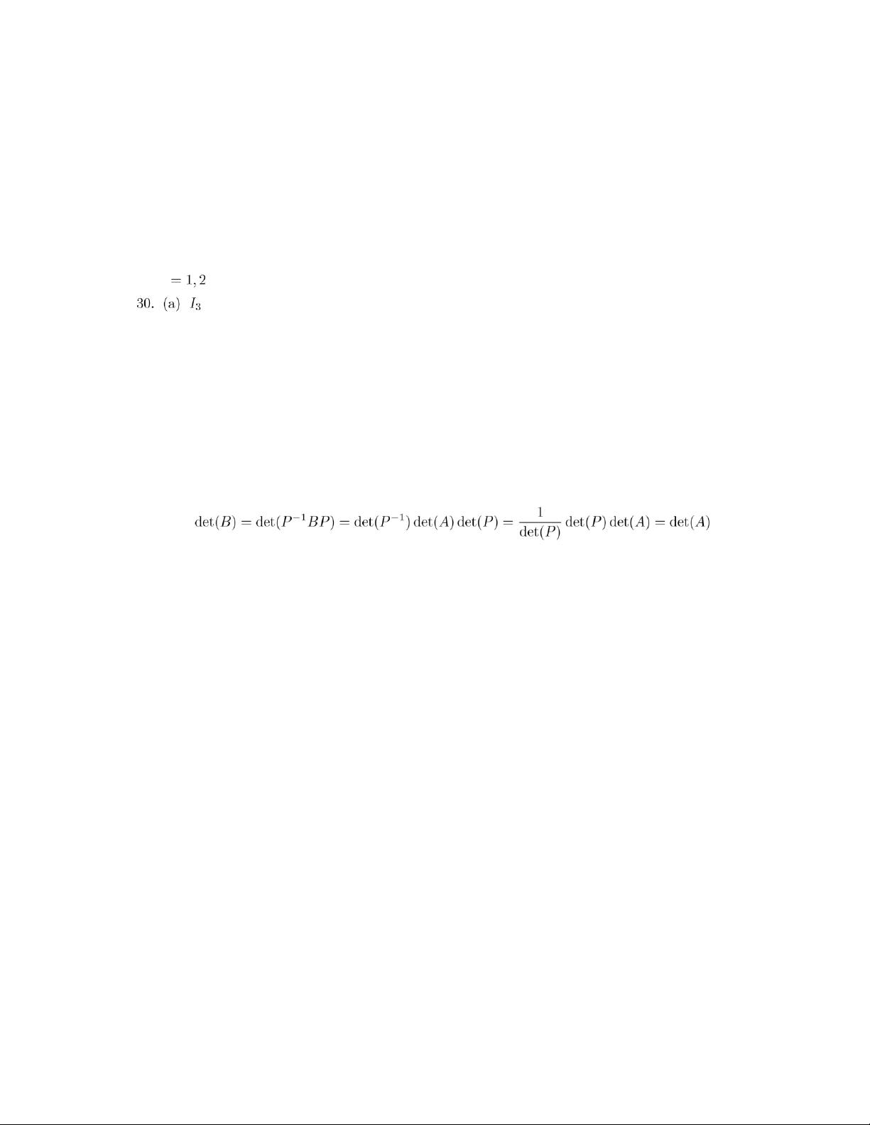
33. If A and B are similar, then there exists a nonsingular matrix P such that B = P−1AP. Then .
34. If det(A) &= 0, then A is nonsingular. Hence, A−1AB = A−1AC, so B = C.
36. In Matlab the command for the determinant actually invokes an LU-factorization, hence is closely
associated with the material in Section 2.5.
37. For−3.2026ǫ = 10×−105,−Matlab14; for ǫ = 10gives the determinant as−15, −6.2800 × 10⁻¹⁵−; for3×10ǫ −=
105 which agrees with the theory; for−16, zero. ǫ = 10−14, Section 3.3, p. 164 2. (a) −23. (b) 7. (c) 15. (d) −28. 4. (a) −3. (b) 0. (c) 3. (d) 6. 6. (b) 2. (c) 24. (f) −30.
8. (b) −24. (d) 72. (e) −120.
9. We proceed by successive expansions along first columns: lOMoAR cPSD| 35974769 51 .
13. (a) From Definition 3.2 each term in the expansion of the determinant of an n×n matrix is a product of n
entries of the matrix. Each of these products contains exactly one entry from each row and exactly one
entry from each column. Thus each such product from det(tIn −A) contains at most n terms of the form t
− aii. Hence each of these products is at most a polynomial of degree n.
Since one of the products has the form (the products is a polynomial of degree n tin−t.a11)(t − a22)···(t − ann) it follows that the sum of
(b) The coefficient of tn is 1 since it only appears in the term (t − a11)(t − a22)···(t − ann) which we
discussed in part (a). (The permutation of the column indices is even here so a plus sign is associated with this term.)
(c) Using part (a), suppose that
det(tIn − A) = tn + c1tn−1 + c2tn−2 + ··· + cn−1t + cn.
Set t = 0 and we have det(−A) = cn which implies that cn = (−1)n det(A). (See Exercise 10 in Section 6.2.)
14. (a) f(t) = t2 − 5t − 2, det(A) = −2.
(b) f(t) = t3 − t2 − 13t − 26, det(A) = 26.
(c) f(t) = t2 − 2t, det(A) = 0. 16. 6.
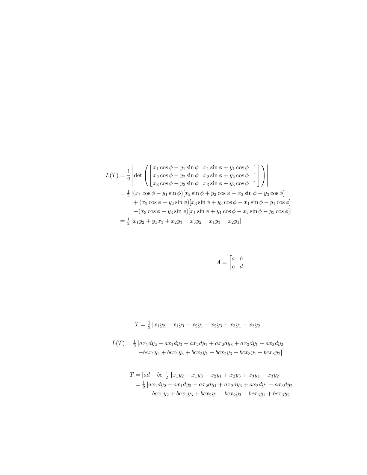
18. Let P1(x1,y1), P2(x2,y2), P3(x3,y3) be the vertices of a triangle T. Then from Equation (2), we have area of .
Let A be the matrix representing a counterclockwise rotation?
L through an angle φ. Thus ( and
are the vertices of L(T), the image of T. We have lOMoAR cPSD| 35974769 52 Chapter 3
2 L'x1(3 = 'x1 cosφ − y1 sinφ(, y1 2 '
x1 sinφ + y1 cosφ 2 Lx2(3 = 'x2
cosφ − y2 sinφ(, y2
x2 sinφ + y2 cosφ
L'x3(3 = 'x3 cosφ − y3 sinφ(, y3
x3 sinφ + y3 cosφ Then area of − − − = area of T.
19. Let T be the triangle with vertices (x1,y1), (x2,y2), and (x3,y3). Let (
Section 3.4 and define the linear operator L: R2 → R2 by L(v) = Av for v in R2. The vertices of L(T) are
(ax1 + by1,cx1 + dy1),
(ax2 + by2,cx2 + dy2), and
(ax3 + by3,cx3 + dy3). Then by Equation (2), Area of and Area of Now, |det(A)| · Area of − − − |
= |Area of L(T)| lOMoAR cPSD| 35974769 53 Section 3.4, p. 169 2. (a) 4.
6. If A is symmetric, then for each i and j, Mji is the transpose of Mij. Thus Aji = (−1)j+i|Mji| = (−1)i+j|Mij| = Aij.
8. The adjoint matrix is upper triangular if A is upper triangular, since aij = 0 if i > j which implies that Aij = 0 if i > j. .
13. We follow the hint. If A is singular then det(A) = 0. Hence A(adj A) = det(A)In = 0In = O. If adj A were
nonsingular, (adj A)−1 exists. Then we have
A(adj A)(adj A)−1 = A = O(adj A)−1 = O,
that is, A = O. But the adjoint of the zero matrix must be a matrix of all zeros. Thus adj A = O so adj A is
singular. This is a contradiction. Hence it follows that adj A is singular.
14. If A is singular, then adj A is also singular by Exercise 13, and det(adjA) = 0 = [det(A)]n−1. If A is nonsingular,
then A(adjA) = det(A)In. Taking the determinant on each side,
det(A)det(adjA) = det(det(A)In) = [det(A)]n.
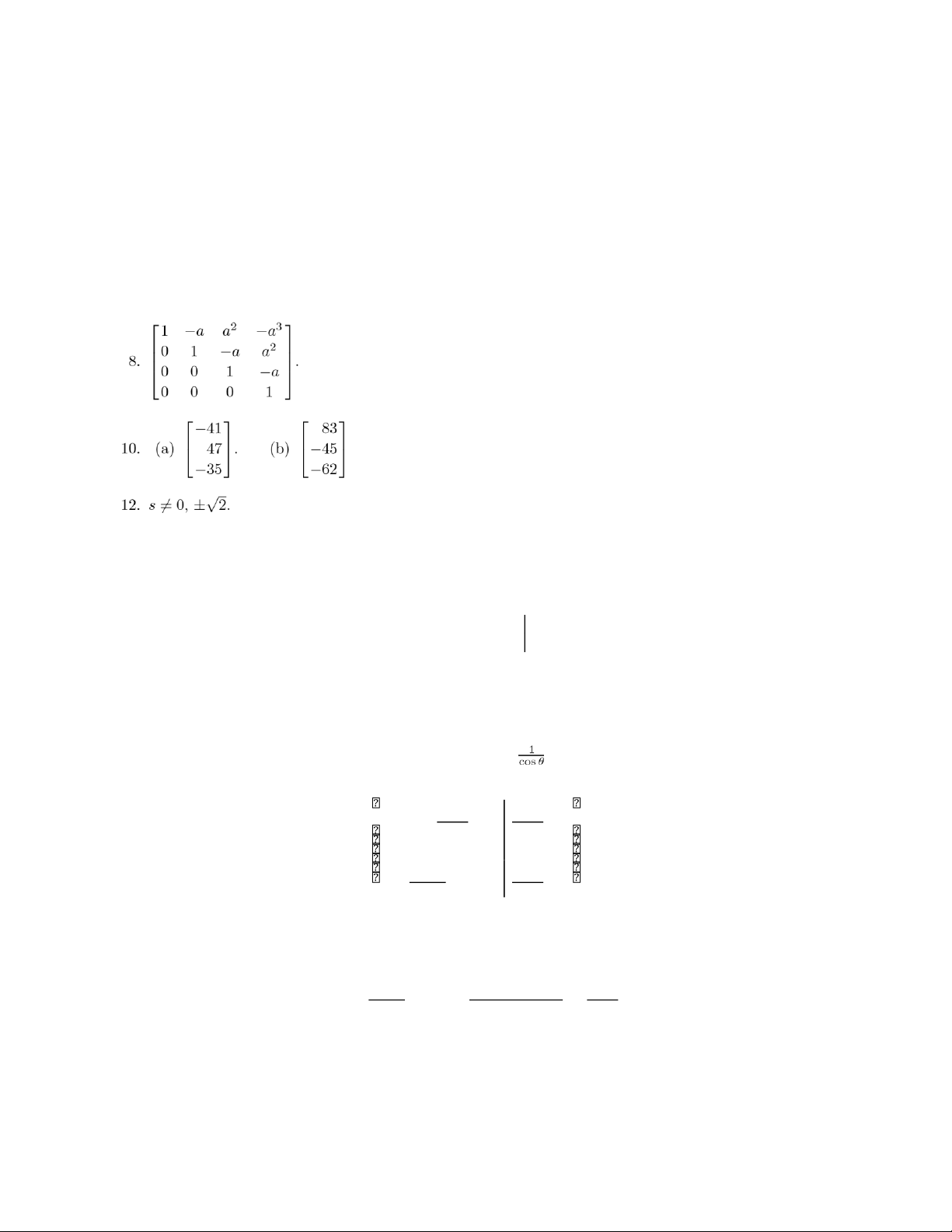
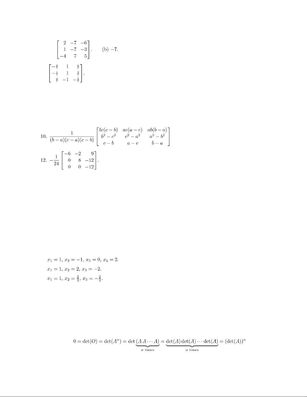
Thus det(adjA) = [det(A)]n−1. Section 3.5, p. 172 2. 4. 6.
Supplementary Exercises for Chapter 3, p. 174 2. (a) t = 1, 4.
(b) t = 3, 4, −1. (c) t = 1, 2, 3. (d) t = −3, 1, −1.
3. If An = O for some positive integer n, then . lOMoAR cPSD| 35974769 54 Chapter 3
It follows that det(A) = 0. 4. (a)
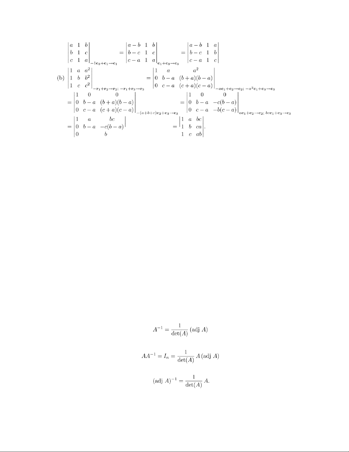
c − a − (c − a)???r1+r2→r2; r1+r3→r3 ???
5. If A is an n × n matrix then
det(AAT) = det(A) det(AT) = det(A) det(A) = (det(A))2.
(Here we used Theorems 3.9 and 3.1.) Since the square of any real number is ≥ 0 we have det(AAT) ≥ 0.
6. The determinant is not a linear transformation from Rnn to R1 for n > 1 since for an arbitrary scalar c,
det(cA) = cn det(A) &= cdet(A).
7. Since A is nonsingular, Corollary 3.4 implies that .
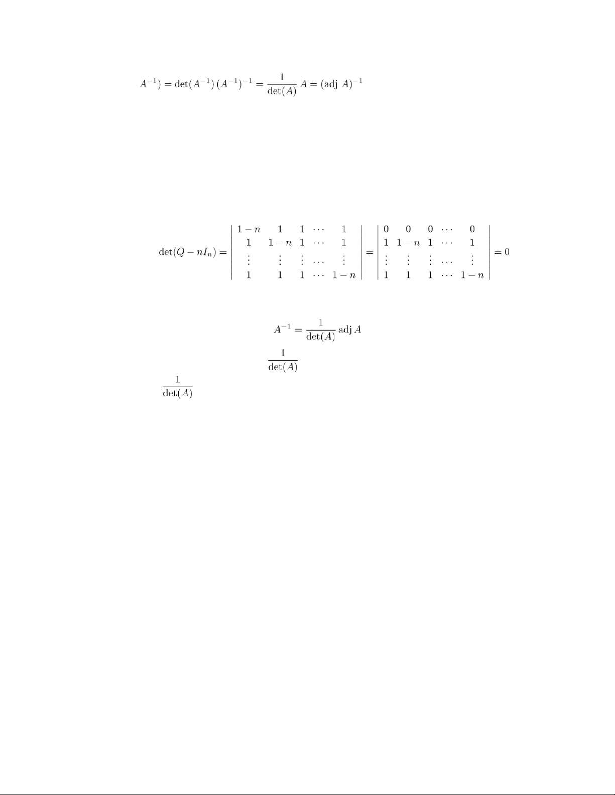
Multiplying both sides on the left by A gives . Hence we have that lOMoAR cPSD| 35974769 55
From Corollary 3.4 it follows that for any nonsingular matrix B, adj B = det(B)B−1. Let B = A−1 and we have adj ( . Chapter Review
8. If rows i and j are proportional with taik = ajk, k = 1,2,...,n, then
det(A) = det(A)−tri+rj→rj = 0
since this row operation makes row j all zeros.
9. Matrix Q is n×n with each entry equal to 1. Then, adding row j to row 1 for j = 2, 3, ..., n, we have by Theorem 3.4.
10. If A has integer entries then the cofactors of A are integers and adj A has only integer entries. If A is nonsingular and
has integer entries it must follow that
times each entry of adj A is an integer. Since adj A has integer entries
must be an integer, so det(A) = ±1. Conversely, if det(A) = ±1, then A is nonsingular
and A−1 = ±1adjA implies that A−1 has integer entries.
11. If A and b have integer entries and det(A) = ±1, then using Cramer’s rule to solve Ax = b, we find that the
numerator in the fraction giving xi is an integer and the denominator is ±1, so xi is an integer for i = 1, 2, ..., n.
Chapter Review for Chapter 3, p. 174 True or False 1. False. 2. True. 3. False. 4. True. 5. True. 6. False. 7. False. 8. True. 9. True. 10. False. 11. True. 12. False. Quiz 1. −54. 2. False. 3. −1. 4. −2.
5. Let the diagonal entries of A be d11,...,dnn. Then det(A) = d11 ···dnn. Since A is singular if and only if det(A) =
0, A is singular if and only if some diagonal entry dii is zero. lOMoAR cPSD| 35974769 56 Chapter 3 6. 19. 7. .
8. det(A) = 14. Therefore . lOMoAR cPSD| 35974769 Chapter 4 Real Vector Spaces Section 4.1, p. 187 2.( − 5 , 7). y ( − 5 , 7) 7 5 3 ( − 3 , 2) 1 x − 5 − 3 − 1 1 3 5
4.(1 , − 6 , 3).
6. a = −2, b = −2, c = −5. 8. (a) '−−24(. (b) −−036 . 10. (a) '−47(. (b) 23 . −3 3 − −6 12. (a) u + v =2 , 2u − v = 045 , 3u − 2v = 167 , 0 − 3v = 03 . 4 − lOMoAR cPSD| 35974769 58 Chapter 4 b) u + v = 131 , 2u v = 1134 , 3u 2v = 1874 , 0 3v = −36 ( − − − − − −9 . .
16. c1 = 1, c2 = −2. 18. Impossible.
20. c1 = r, c2 = s, c3 = t. 22. If u , then ( .
23. Parts 2–8 of Theorem 4.1 require that we show equality of certain vectors. Since the vectors are
columnmatrices, this is equivalent to showing that corresponding entries of the matrices involved are
equal. Hence instead of displaying the matrices we need only work with the matrix entries. Suppose u, v,
w are in R3 with c and d real scalars. It follows that all the components of matrices involved will be real
numbers, hence when appropriate we will use properties of real numbers. (2)
(u + (v + w))i = ui + (vi + wi)
((u + v) + w)i = (ui + vi) + wi
Since real numbers ui + (vi + wi) and (ui + vi) + wi are equal for i = 1, 2, 3 we have u + (v + w) = (u + v) + w. (3)
(u + 0)i = ui + 0
(0 + u)i = 0 + ui
(u)i = ui
Since real numbers ui + 0, 0 + ui, and ui are equal for i = 1, 2, 3 we have u + 0 = 0 + u = u.
Since real numbers ui + (−ui) and 0 are equal for i = 1, 2, 3 we have u + (−u) = 0. (5)
(c(u + v))i = c(ui + vi)
(cu + cv)i = cui + cvi
Since real numbers c(ui + vi) and cui + cvi are equal for i = 1, 2, 3 we have c(u + v) = cu + cv. (6)
((c + d)u)i = (c + d)ui
(cu + du)i = cui + dui
Since real numbers (c + d)ui and cui + dui are equal for i = 1, 2, 3 we have (c + d)u = cu + du. (7)
(c(du))i = c(dui)
((cd)u)i = (cd)ui lOMoAR cPSD| 35974769
Since real numbers c(dui) and (cd)ui are equal for i = 1, 2, 3 we have c(du) = (cd)u. (8)
(1u)i = 1ui
(u)i = ui
Since real numbers 1ui and ui are equal for i = 1, 2, 3 we have 1u = u.
The proof for vectors in R2 is obtained by letting i be only 1 and 2. lOMoAR cPSD| 35974769 60 Chapter 4 Section 4.2 Section 4.2, p. 196
1. (a) The polynomials t2 + t and −t2 − 1 are in P2, but their sum (t2 + t) + (−t2 − 1) = t − 1 is not in P2.
(b) No, since 0(t2 + 1) = 0 is not in P2. 2. (a) No. (b) Yes. . (d) Yes. If , then abcd = 0. Let (. Then ( and
−A ∈ V since (−a)(−b)(−c)(−d) = 0.
(e) No. V is not closed under scalar multiplication.
4. No, since V is not closed under scalar multiplication. For example, v , but . 5. Let u .
(1) For each i = 1,...,n, the ith component of u + v is ui + vi, which equals the ith component vi + ui of v + u.
(2) For each i = 1,...,n, ui + (vi + wi) = (ui + vi) + wi.
(3) For each i = 1,...,n, ui + 0 = 0 + ui = ui. (4) For each (5) For each
(6) For each i = 1,...,n, (c + d)ui = cui + dui.
(7) For each i = 1,...,n, c(dui) = (cd)ui.
(8) For each i = 1,...,n, 1 · ui = ui.
6. P is a vector space.
(a) Let p(t) and q(t) be polynomials not both zero. Suppose the larger of their degrees is n. Then p(t) +
q(t) and cp(t) are computed as in Example 5. The properties of Definition 4.4 are verified as in Example 5. 8. Property 6. 10. Properties 4 and (b).
12. The vector 0 is the real number 1, and if u is a vector (that is, a positive real number) then u .
13. The vector 0 in V is the constant zero function. lOMoAR cPSD| 35974769 61
14. Verify the properties in Definition 4.4.
15. Verify the properties in Definition 4.4. 16. No.
17. No. The zero element for ⊕= 1would have to be the real number 1, but then. Thus (4) fails to hold. (5)
fails since c .u(= 0u ⊕has no “negative”v) = c + (uv) &= v such that u ⊕ v = 0 · v
(c + u)(c + v) = c . u ⊕ c . v. Etc.
18. No. For example, (1) fails since 2u − v &= 2v − u.
19. Let 01 and 02 be zero vectors. Then 01 ⊕ 02 = 01 and 01 ⊕ 02 = 02. So 01 = 02.
20. Let u1 and u2 be negatives of u. Then u ⊕ u1 = 0 and u ⊕ u2 = 0. So u ⊕ u1 = u ⊕ u2. Then
u1 ⊕ (u ⊕ u1) = u1 ⊕ (u ⊕ u2)
(u1 ⊕ u) ⊕ u1 = (u1 ⊕ u) ⊕ u2
0 ⊕ u1 = 0 ⊕ u2 u1 = u2.
21. (b) c . 0 = c . (0 ⊕ 0) = c . 0 ⊕ c . 0 so c . 0 = 0.
(c Letso uc=.u0.= 0. If c = 0& , then 1c .(c.u) = 1c .0 = 0. Now 1c .(c.u) = 091c:(c)1.u = 1.u = u,
22. Verify as for Exercise 9. Also, each continuous function is a real valued function.
23. v ⊕ (−v) = 0, so −(−v) = v.
24. If u ⊕ v = u ⊕ w, add −u to both sides.
25. If a . u = b . u, then (a − b) . u = 0. Now use (c) of Theorem 4.2. Section 4.3, p. 205 2. Yes. 4. No. 6. (a) and (c). 8. (a). 10. (c). 12. (a) Let and lOMoAR cPSD| 35974769 62 Chapter 4
be any vectors in W. Then
is in W. Moreover, if k is a scalar, then
is in W. Hence, W is a subspace of M33. Section 4.3
Alternate solution: Observe that every vector in W can be written as ,
so W consists of all linear combinations of five fixed vectors in M33. Hence, W is a subspace of M33. 14. We have ,
so A is in W if and only if a + b = 0 and c + d = 0. Thus, W consists of all matrices of the form . Now if ( and ( are in W, then (
is in W. Moreover, if k is a scalar, then (
is in W. Alternatively, we can observe that every vector in W can be written as ,
so W consists of all linear combinations of two fixed vectors in M22. Hence, W is a subspace of M22. 16. (a) and (b). 18. (b) and (c). 20. (a), (b), (c), and (d). lOMoAR cPSD| 35974769 63 21. Use Theorem 4.3. 22. Use Theorem 4.3.
23. Let x1 and x2 be solutions to Ax = b. Then A(x1 + x2) = Ax1 + Ax2 = b + b =& b if b &= 0. 24. {0}. 25. Since , it follows that
is in the null space of A.
26. We have cx0 + dx0 = (c + d)x0 is in W, and if r is a scalar then r(cx0) = (rc)x0 is in W.
27. No, it is not a subspace. Let x be in W so Ax =& 0. Letting y = −x, we have y is also in W and Ay =& 0.
However, A(x + y) = 0, so x + y does not belong to W.
28. Let V be a subspace of R1 which is not the zero subspace and let v =& 0 be any vector in V . If u is any
nonzero vector in R1, then u
v, so R1 is a subset of V . Hence, V = R1.
29. Certainly {0} and R2 are subspaces of R2. If u is any nonzero vector then span {u} is a subspace of R2. To
show this, observe that span {u} consists of all vectors in R2 that are scalar multiples of u. Let v = cu and
w = du be in span {u} where c and d are any real numbers. Then v+w = cu+du = (c+d)u is in span {u} and
if k is any real number, then kv = k(cu) = (kc)u is in span {u}. Then by Theorem 4.3, span {u} is a subspace of R2.
To show that these are the only subspaces of R2 we proceed as follows. Let W be any subspace of R2. Since
W is a vector space in its own right, it contains the zero vector 0. If W =& {0}, then W contains a nonzero
vector u. But then by property (b) of Definition 4.4, W must contain every scalar multiple of u. If every
vector in W is a scalar multiple of u then W is span {u}. Otherwise, W contains span {u} and another vector
which is not a multiple of u. Call this other vector v. It follows that W contains span {u,v}. But in fact span
{u,v} = R2. To show this, let y be any vector in R2 and let u , and y .
We must show there are scalars c1 and c2 such that c1u + c2v = y. This equation leads to the linear system .
Consider the transpose of the coefficient matrix: . lOMoAR cPSD| 35974769 64 Chapter 4
This matrix is row equivalent to I2 since its rows are not multiples of each other. Therefore the matrix is
nonsingular. It follows that the coefficient matrix is nonsingular and hence the linear system has a
solution. Therefore span {u,v} = R2, as required, and hence the only subspaces of R2 are {0}, R2, or scalar
multiples of a single nonzero vector.
30. (b) Use Exercise 25. The depicted set represents all scalar multiples of a nonzero vector, hence is a subspace. 31. We have ' .
32. Every vector in W is of the form(, which can be written as a b b c , where v , and v . 34. (a) and (c). Section 4.4
35. (a) The line l0 consists of all vectors of the form . Use Theorem 4.3.
(b) The line l through the point P0(x0,y0,z0) consists of all vectors of the form .
If P0 is not the origin, the conditions of Theorem 4.3 are not satisfied. 36. (d)
38. (a) x = 3 + 4t, y = 4 − 5t, z = −2 + 2t.
(b) x = 3 − 2t, y = 2 + 5t, z = 4 + t.
42. Use matrix multiplication cA where c is a row vector containing the coefficients and matrix A has rows
that are the vectors from Rn. Section 4.4, p. 215
2. (a) 1 does not belong to span S. lOMoAR cPSD| 35974769 65
(b) Span S consists of all vectors of the form
is any real number. Thus, the vector ( is not in span S.
(c) Span S consists of all vectors of M22 of the form
(, where a and b are any real numbers. Thus, the vector ( is not in span S. 4. (a) Yes. (b) Yes. (c) No. (d) No. 6. (d). 8. (a) and (c). 10. Yes. .
13. Every vector A in W is of the form
(, where a, b, and c are any real numbers. We have ,
so A is in span S. Thus, every vector in W is in span S. Hence, span S = W. 1 0 0 0 1 0 0 0 1 0 0 0 0 0 0 0 0 0 14. S =0 0 0 , 0 0 0 , 0 0 0 , 1 0 0 , 0 1 0 , 0 0 1 , 0 0 −1 0 0 0 0 0 0 0 0 0 0 0 −1 0 0 0 0 0 0 0 0 0 1 0 0 0 1 0 0 0 0 , 0 0 0 . lOMoAR cPSD| 35974769 66 Chapter 4
16. From Exercise 43 in Section 1.3, we have Tr(AB) = Tr(BA), and Tr(AB−BA) = Tr(AB)−STr(is a properBA) =
0. Hence, span T is a subset of the set S of all n × n matrices with trace = 0. However, subset of Mnn. Section 4.5, p. 226 1. We form Equation (1): ,
which has nontrivial solutions. Hence, S is linearly dependent. 2. We form Equation (1): ,
which has only the trivial solution. Hence, S is linearly independent. 4. No. 6. Linearly dependent. 8. Linearly independent. 10. Yes.
12. (b) and (c) are linearly independent, (a) is linearly dependent. .
14. Only (d) is linearly dependent: cos2t = cos2 t − sin2 t. 16. c = 1.
18. Suppose that {u,v} is linearly dependent. Then c1u + c2v = 0, where c1 and c2 are not both zero. Say c2 &= 0. Then v
u. Conversely, if v = ku, then ku−1v = 0. Since the coefficient of v is nonzero, {u,v} is linearly dependent.
19. Let S = {v1,v2,...,vak1},abe linearly dependent.
Then2,...,ak is not zero. Say
that j + akvk = 0, where at least one of the coefficients v .
20. Suppose a1w1 + a2w2 1+ a3w31= a21(v1 + v2 + v3) +2a2(v2 + v3) +1 a32v3 =3 0. Since {v1,v2a,3v= 0).3} is linearly
independent, a = 0, a +a = 0 (and hence a = 0), and a +a +a = 0 (and hence
Thus {w1,w2,w3} is linearly independent. Section 4.5
21. Form the linear combination lOMoAR cPSD| 35974769 67
c1w1 + c2w2 + c3w3 = 0
which gives c1(v1 + v2) + c2(v1 + v3) + c3(v2 + v3) = (c1 + c2)v1 + (c1 + c3)v2 + (c2 + c3)v3 = 0. Since S is linearly independent we have
c1 + c2 = 0 c1 + c3
= 0 c2 + c3 = 0 0 1 10 1 1 00
a linear system whose augmented matrix is1 0 10
. The reduced row echelon form is 1 0 00 0 1 00 0 0 10
thus c1 = c2 = c3 = 0 which implies that {w1,w2,w3} is linearly independent.
22. Form the linear combination
c1w1 + c2w2 + c3w3 = 0
which gives c1v1 + c2(v1 + v3) + c3(v1 + v2 + v3) = (c1 + c2 + c3)v1 + (c2 + c3)v2 + c3v3 = 0.
Since S is linearly dependent, this last equation is satisfied with c1 + c2 + c3, c3, and c2 + c3 not all being zero.
This implies that c1, c2, and c3 are not all zero. Hence, {w1,w2,w3} is linearly dependent.
23. Suppose {v1,v2,v3} is linearly dependent. Then one of the vj’s is a linear combination of the preceding
vectors in the list. It must be v3 since {v1,v2} is linearly independent. Thus v3 belongs to span {v1,v2}. Contradiction.
24. Form the linear combination
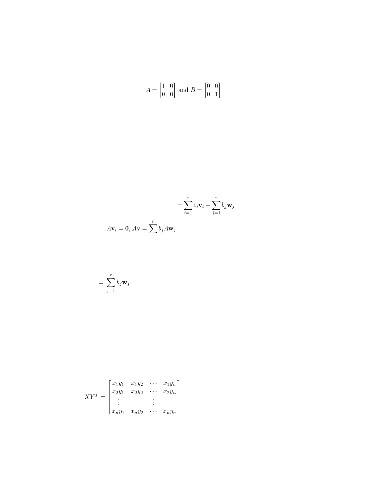
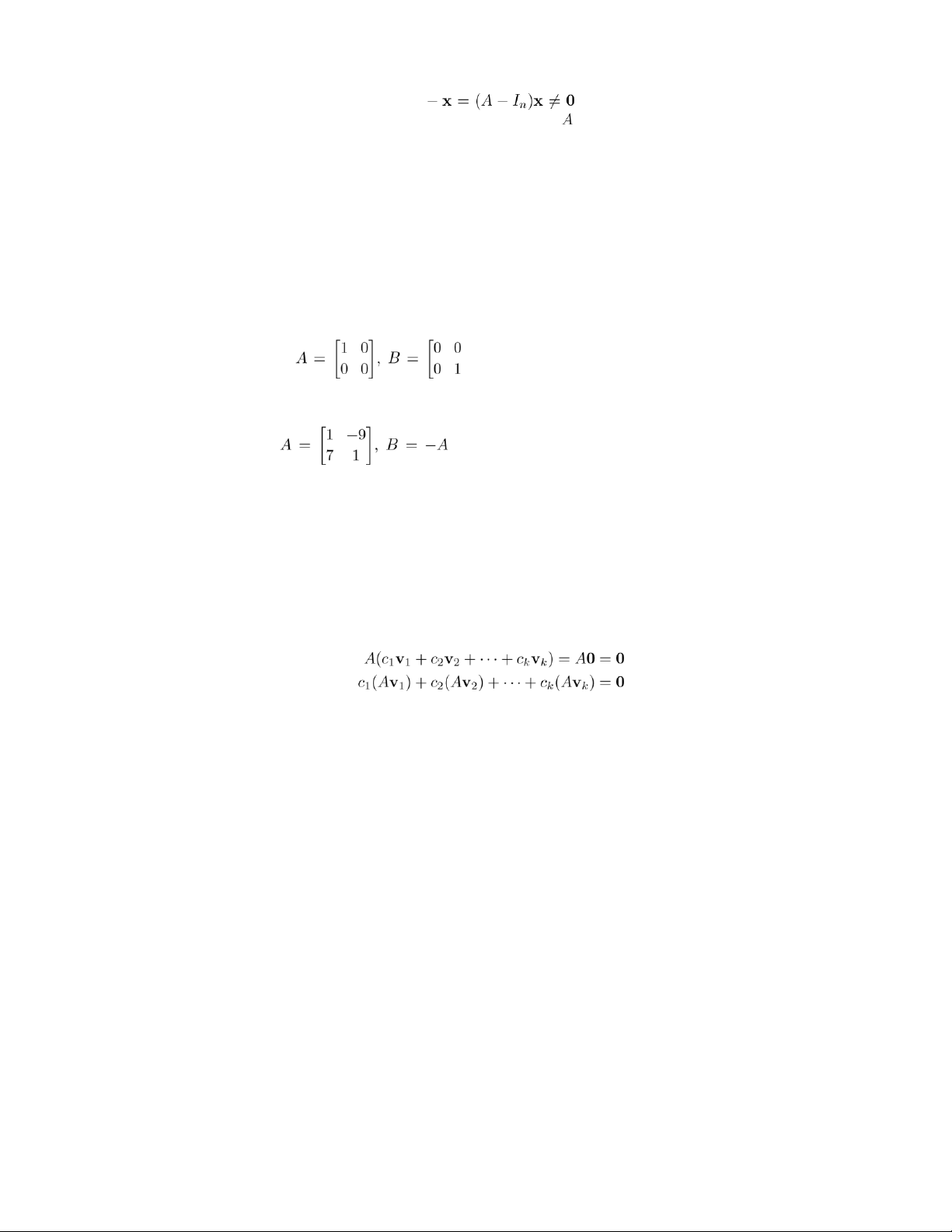
c1Av1 + c2Av2 + ··· + cnAvn = A(c1v1 + c2v2 + ··· + cnvn) = 0.
Since A is nonsingular, Theorem 2.9 implies that
c1v1 + c2v2 + ··· + cnvn = 0. lOMoAR cPSD| 35974769 68 Chapter 4
Since {v1,v2,...,vn} is linearly independent, we have c1 = c2 = ··· = cn = 0. Hence, {Av1,Av2,. ., Avn} is linearly independent.
25. Let A have k nonzero rows, which we denote by v1,v2,...,vk where
vi = 0ai1 ai2
··· 1 ··· ain1.
Let c1 < c2 < ··· < ck be the columns in which the leading entries of the k nonzero rows occur. Thus vi = 00 0
0 ··· 1 aici+1 ··· ain1 that is, aij = 0 for j < ci and cici = 1. If a1v1 + a2v2 + ··· + akvk = 00 0 ··· 01, examining the c1th
entry on the left yields a1 = 0, examining the c2th entry yields a2 = 0, and so forth. Therefore v1,v2,...,vk are linearly independent. 26. Let v . Then w .
27. In R1 let S1 = {1} and S2 = {1,0}. S1 is linearly independent and S2 is linearly dependent. 28. See Exercise 27 above.
29. In Matlab the command null(A) produces an orthonormal basis for the null space of A.
31. Each set of two vectors is linearly independent since they are not scalar multiples of one another. In Matlab
the reduced row echelon form command implies sets (a) and (b) are linearly independent while (c) is linearly dependent. Section 4.6, p. 242 2. (c). 4. (d). (. The
first three entries implyci
c3 = −c1 = c4 = −c2. The fourth entry gives c2 − c2 − c2 = −c2 = 0. Thus
= 0 for i = 1, 2, 3, 4. Hence the set of four matrices is linearly independent. By Theorem 4.12, it is a basis. 8. (b) is a basis for .
10. (a) forms a basis: 5t2 − 3t + 8 = −3(t2 + t) + 0t2 + 8(t2 + 1). lOMoAR cPSD| 35974769 69
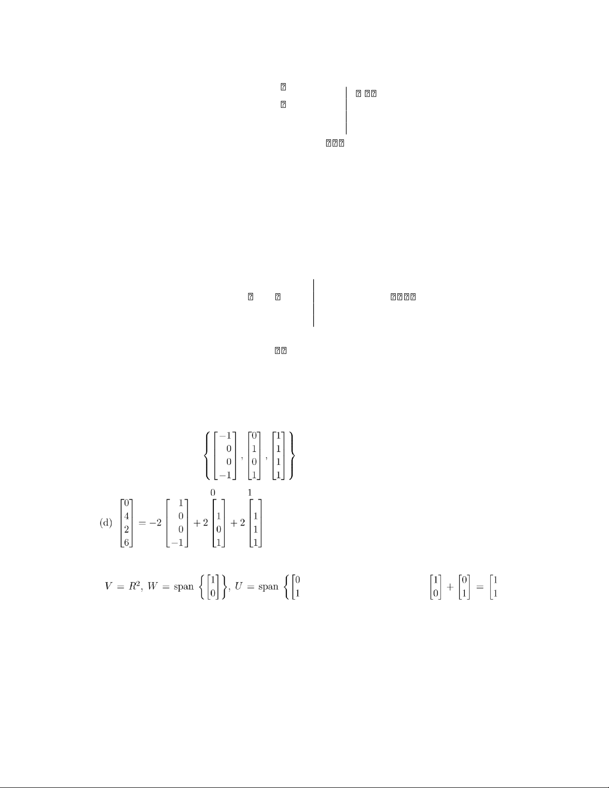
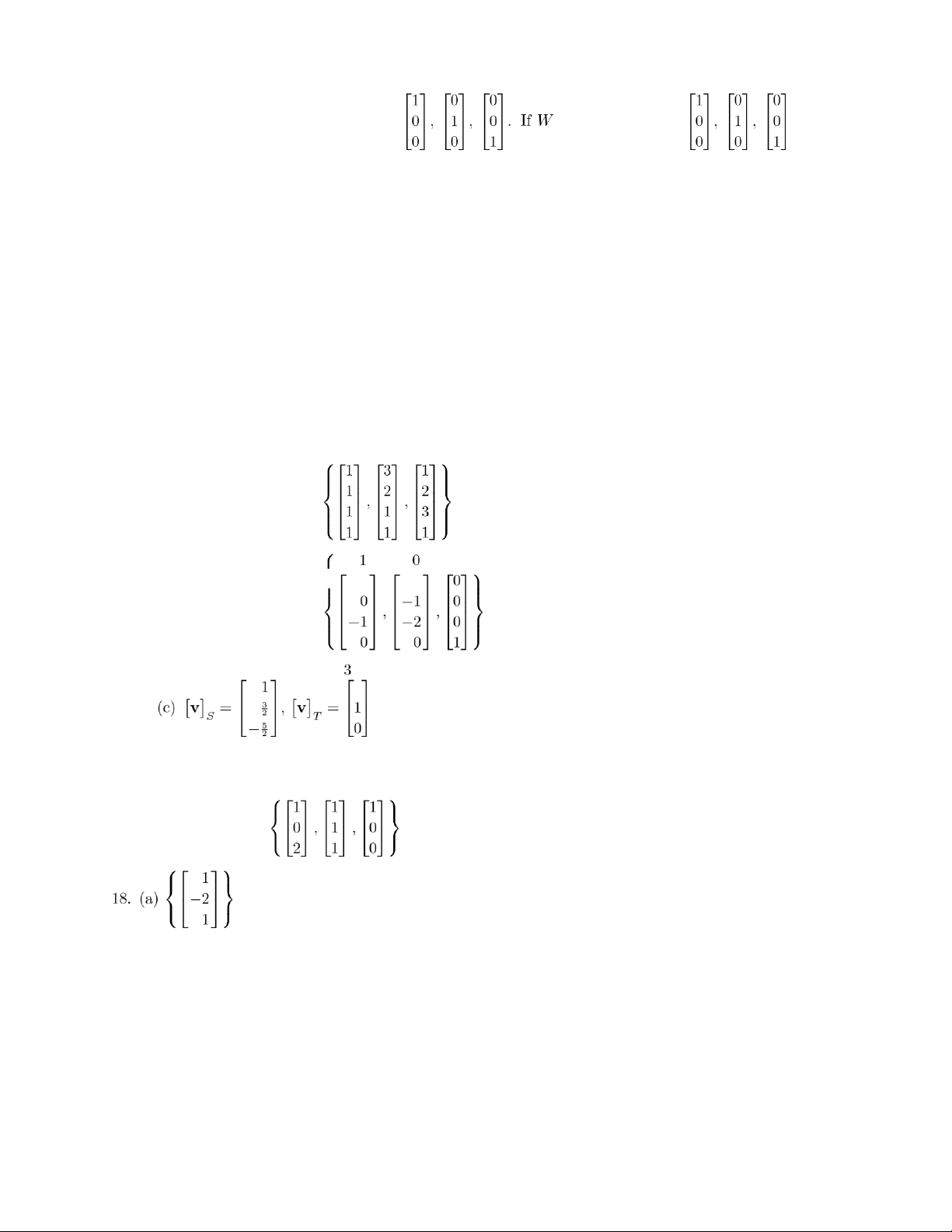
12. A possible answer is G01 1 0 −11,00 1 2 11,00 0 3 11H; dimW = 3. 14. I' (,' (J. 1 0 0 1 0 1 1 0 1 0 0 0 1 0 0 0 1 0 0 0 0 0 0 0 0 0
16.0 0 0 , 1 0 0 , 0 0 0 , 0 1 0 , 0 0 1 , 0 0 0 . 0 0 0 0 0 0 2 1 0 02 0 0 0 0 1 0 0 0 1
18. A possible answer is {cos t,sin t} is a basis for W; dimW = 2. . 28. (a) A possible answer is . (b) A possible answer is . Section 4.6 (J;
dimM23 = 6. dimMmn = mn. 32. 2.
34. The set of all polynomials of the form at3 + bt2 + (b − a), where a and b are any real numbers.
35. We show that {cv1,v2,...,vk} is also a set of k = dimV vectors which spans V . If v is a vector in V , then v . lOMoAR cPSD| 35974769 70 Chapter 4
36. Let d = max{d1,d2,...,dk}. The polynomial td+1 + td + ··· + t + 1 cannot be written as a linear combination of
polynomials of degrees ≤ d.
37. If dimV = n, then V has a basis consisting of n vectors. Theorem 4.10 then implies the result.
38. Let S = {v1,v2,...,vk} be a minimal spanning set for V . From Theorem 4.9, S contains a basis T for V . Since
T spans S and S is a spanning set for V , T = S. It follows from Corollary 4.1 that k = n.
39. Let T = {v1,v2,...,vm}, m > n be a set of vectors in V . Since m > n, Theorem 4.10 implies that T is linearly dependent.
40. Let dimV = n and let S be a set of vectors in V containing m elements, m < n. Assume that S spans V . By
Theorem 4.9, S contains a basis T for V . Then T must contain n elements. This contradiction implies that
S cannot span V .
41. Let dimV = n. First observe that any set of vectors in W that is linearly independent in W is linearly
independent in V . If W = {0}, then dimW = 0 and we are done. Suppose now that W is a nonzero subspace
of V . Then W contains a nonzero vector v1, so {v1} is linearly independent in W (and in V ). If span {v1} =
W, then dimW = 1 and we are done. If span {v1} =& W, then there exists a vector v2 in W which is not in
span {v1}. Then {v1,v2} is linearly independent in W (and in V ). Since dimV = n, no linearly independent
set of vectors in V can have more than n vectors. Hence, no linearly independent set of vectors in W can
have more than n vectors. Continuing the above process we find a basis for W containing at most n
vectors. Hence dimW ≤ dimV .
42. Let dimV = dimW = n. Let S = {v1,v2,...,vn} be a basis for W. Then S is also a basis for V , by Theorem 4.13. Hence, V = W.
43. Let V = R3. The trivial subspaces of any vector space are {0} and V . Hence {0} and R3 are subspaces of R3.
In Exercise 35 in Section 4.3 we showed that any line % through the origin is a subspace of R3. Thus we
need only show that any plane π passing through the origin is a subspace of R3. Any plane π in R3 through
the origin has an equation of the form ax+by +cz = 0. Sums and scalar multiples of any point on π will
also satisfy this equation, hence π is a subspace of R3. To show that {0}, V , lines, and planes through the
origin are the only subspaces of R3 we argue in a manner similar to that given in Exercise 29 in Section
4.3 which considered a similar problem in R2. Let W be any subspace of R3. Hence W contains the zero
vector 0. If W =& {0} then it contains a nonzero vector v{=}0a b c1 T
where at least one of a, b, or c is not zero. Since W is a subspace it contains span v . If W = span {v} then
W is a line in R3 through the origin. Otherwise, there exists a vector u in W which is not in span {v}. Hence
{v,u} is a linearly independent set. But then W contains span {v,u}. If W = span {v,u} then W is a plane
through the origin. Otherwise there is a vector x in W that is not in span {v,u}. Hence {v,u,x} is a linearly
independent set in W and W contains span {v,u,x}. But {v,u,x} is a maximal linearly independent set in R3,
hence a basis for R3. It follows in this case that W = R3. lOMoAR cPSD| 35974769 71
44. Let S = {v1,v2,...,vn}. Since every vector in V can be written as a linear combination of the vectors in S, it
follows that S spans V . Suppose now that
a1v1 + a2v2 + ··· + anvn = 0. We also have
0v1 + 0v2 + ··· + 0vn = 0.
From the hypothesis it then follows that a1 = 0, a2 = 0, ..., an = 0. Hence, S is a basis for V .
45. (a) If span S =& V , then there exists a vector v in V that is not in S. Vector v cannot be the zero vector
since the zero vector is in every subspace and hence in span S. Hence S1 = {v1,v2,. .,vn,v} is a linearly
independent set. This follows since vi, i = 1,. .,n are linearly independent and v is not a linear combination
of the vi. But this contradicts Corollary 4.4. Hence our assumption that span S =& V is incorrect. Thus
span S = V . Since S is linearly independent and spans V it is a basis for V .
(b) We want to show that S is linearly independent. Suppose S is linearly dependent. Then there is a
subset of S consisting of at most n − 1 vectors which is a basis for V . (This follows from Theorem 4.9)
But this contradicts dimV = n. Hence our assumption is false and S is linearly independent. Since S
spans V and is linearly independent it is a basis for V .
46. Let T = {v1,v2,. .,vk} be a maximal independent subset of S, and let v be any vector in S. Since T is a maximal
independent subset then {v1,v2,. .,vk,v} is linearly dependent, and from Theorem 4.7 it follows that v is a
linear combination of {v1,v2,...,vk}, that is, of the vectors in T. Since S spans V , we find that T also spans V
and is thus a basis for V .
47. If A is nonsingular then the linear system Ax = 0 has only the trivial solution x = 0. Let
c1Av1 + c2Av2 + ··· + cnAvn = 0.
Then A(c1v1 + ··· + cnvn) = 0 and by the opening remark we must have
c1v1 + c2v2 + ··· + cnvn = 0. However since {v =
1,v2,...,vn} is linearly independent it follows that c1 = c2 ··· = cn = 0. Hence {Av1,Av2,...,Avn} is linearly independent.
48. Since A is singular, Theorem 2.9 implies that the homogeneous system Ax = 0 has a nontrivial solution
x. Since {v1,v2,...,vn} is a linearly independent set of vectors in Rn, it is a basis for Rn, so
x = c1v1 + c2v2 + ··· + cnvn. Observe that x =&
0, so c1,c2,...,cn are not all zero. Then
0 = Ax = A(c1v1 + c2v2 + ··· + cnvn) = c1(Av1) + c2(Av2) + ··· + cn(Avn).
Hence, {Av1,Av2,...,Avn} is linearly dependent. lOMoAR cPSD| 35974769 72 Chapter 4 Section 4.7, p. 251 2.
(a) x = −r + 2s, y = r, z = s, where r, s are any real numbers. (b) Let x . Then . Section 4.7 ( c ) z x 1 x 2 y O x 4. ; dimension = 3. 6. ; dimension = 2. 8. No basis; dimension = 0. 10. 0−210000 , 01751000 ; dimension = 2. lOMoAR cPSD| 35974769 73 12. 31103 , −−1630 . 14. I'−1(J. 16. No basis.
22. x = xp + xh, where any number.
23. Since each vector in S is a solution to Ax = 0, we have Axi = 0 for i = 1,2,...,n. The span of S consists of all
possible linear combinations of the vectors in S. Hence
y = c1x1 + c2x2 + ··· + ckxk
represents an arbitrary member of span S. We have
Ay = c1Ax1 + c2Ax2 + ··· + ckAxk = c10 + c20 + ··· + ck0 = 0.
24. If A has a row or column of zeros, then A is singular (Exercise 46 in Section 1.5), so by Theorem 2.9, the
homogeneous system Ax = 0 has a nontrivial solution.
25. (a) Let A = 0aij1. Since the dimension of the null space of1 2 3 A is 3, the null space of1 A 2is R3. Then the3
natural basis {e ,e ,e } is a basis for the null space ofA must be zero. Hence, AA. Forming= O. Ae = 0, Ae =
0, Ae = 0, we find that all the columns of
(b) Since Ax = 0 has a nontrivial solution, the null space of A contains a nonzero vector, so the dimension
of the null space of A is not zero. If this dimension is 3, then by part (a), A = O, a contradiction. Hence,
the dimension is either 1 or 2.
26. Since the reduced row echelon forms of matrices A and B are the same it follows that the solutions to the
linear systems Ax = 0 and Bx = 0 are the same set of vectors. Hence the null spaces of A and B are the same. lOMoAR cPSD| 35974769 74 Chapter 4 Section 4.8, p. 267 3 2.2 . −1 1 4.−1 . 3 −1 2 −2 6.. 4 8. (3,1,3).
10. t2 − 3t + 2. 12. '−1 1(. 2 1
13. (a) To show S is a basis for R2 we show that the set is linearly independent and since dimR2 = 2 we can
conclude they are a basis. The linear combination ( leads to the augmented matrix '(. 1 10 −1 −20 0
The reduced row echelon form of this homogeneous system is 'I2( so the set S is linearly 0 independent. Section 4.8
(b) Find c1 and c2 so that lOMoAR cPSD| 35974769 75 .
The corresponding linear system has augmented matrix (. ' 1 12
−1 −26 The reduced row echelon form is '( so 0v1S = ' (. 1 010 10 0 1−8 −8
(c) Av1 = '−00..33( = −.3'−11( = −0.3v1, so λ1 = −0.3. ' 0.25 1 (d) Av2 =( = 0.25'
( = 0.25v2 so λ2 = 0.25. −.50 −2
(e) v = 10v1 − 8v2 so Anv = 10Anv1 − 8Anv2 = 10(λ1)nv1 − 8(λ2)nv2. (f) As n increases, the limit
of the sequence is the zero vector.
14. (a) Since dimR2 = 2, we show that S is a linearly independent set. The augmented matrix corre- sponding to ( is ' −1 −23
00 (. The reduced row echelon form is 0 I2 0 1 so S is a linearly independent set. 1 (b) Set v .
Solving for c1 and c2 we find c1 = 18 and c2 = 7. Thus .
(c) Av1 = '−1 −2(' 1( = ' 1(, so λ1 = 1. 3 4 −1 −1 ' (d) Av2
=−1 −2('−2( = '−4( = 2'−2(, so λ2 = 2. 3 4 3 6 3 lOMoAR cPSD| 35974769 76 Chapter 4
(e) Anv =An[18v1 + 7v2] = 18Anv1 + 7Anv2 = 18(1)nv1 + 7(2)nv2 = 18v1 + 7(2n)v2.
(f) As n increases the sequence becomes unbounded since limn→∞ Anv = 18v1 + 7v2 limn→∞ 2n. −9 1 0 1 16. (a)vT = −8 , 0w1T = −2 . 28 13 2 −18 0 (c)v1S = 1 , 0w1S = −17 . (d) Same as (c). 3 8 T S −2 1 −2 (e) Q ← =−1 0 −2 . (f) Same as (a). 4 −1 7 4 0 0 1 18. (a)vT = −2 , 0w1T = 8 .(b) . 1 −6 0 1 −2 0 1S 8
(c)vS = 3 , w = −4 . (d) Same as (c). −2 −2 T S 0 1 1 1 2 0 (e) Q ← = r1 0 0 . (f) Same as (a). 5 20. ' (. 3 4 22.−1 . 3 lOMoAR cPSD| 35974769 77 3 2 3 24. T = 2 , 1 , 1 . 0 0 3
26. T = I' (,' (J. 2 1 5 3
28. (a) V is isomorphic to itself. Let L: V → V be defined by L(v) = v for v in V ; that is, L is the identity map.
(b) If V is isomorphic to W1, then there is an isomorphism L1 : V → W which is a one-to-one and onto
mapping. Thenisomorphism. This is all done in the proof of Theorem 6.7.L− : W → V exists. Verify
that L− is one-to-one and onto and is also an
(c) IfL2U: Vis isomorphic to→ W be an isomorphism. LetV , let L1 : U →L:VU be an isomorphism.→ W be
defined by LIf(vV) =is isomorphic toL2(L1(v)) for vWin, letU.
Verify that L is an isomorphism.
29. (a) L(0V ) = L(0V + 0V ) = L(0V ) + L(0V ), so L(0V ) = 0W.
(b) L(v − w) = L(v + (−1)w) = L(v) + L((−1)w) = L(v) + (−1)L(w) = L(v) − L(w).
30. By Theorem 3.15, Rn and Rm are isomorphic if and only if their dimensions are equal.
31. Let L: Rn → Rn be defined by .
Verify that L is an isomorphism.
32. Let L: P2 → R3 be defined by
. Verify that L is an isomorphism.
33. (a) Let L: M22 → R4 be defined by .
Verify that L is an isomorphism. Section 4.8 lOMoAR cPSD| 35974769 78 Chapter 4 (b) dimM22 = 4.
34. If v is any vector in V , then v = aet +be−t, where a and b are scalars. Then let L: V → R2 be defined by
(. Verify that L is an isomorphism.
35. From Exercise 18 in Section 4.6, V = span S has a basis {sin2 t,cos2 t} hence dimV = 2. It follows from
Theorem 4.14 that V is isomorphic to R2.
36. Let V and W be isomorphic under the isomorphism L. If V1 is a subspace of V then W1 = L(V ) is a subspace
of W which is isomorphic to V1.
37. Let v = w. The coordinates of a vector relative to basis S are the coefficients used to express the vector
in terms of the members of S. A vector has a unique expression in terms of the vectors of a basis, hence
it follows that 0v1S must equal 0w1S. Conversely, let .
then v = a1v1 + a2v2 + ··· + anvn and w = a1v1 + a2v2 + ··· + anvn. Hence v = w.
38. Let S = {v1,v2,...,vn} and v = a1v1 + a2v2 + ··· + anvn, w = b1v1 + b2v2 + ··· + bnvn. Then and . We also have v so 0 1
v + w S = n12 ... n12 = ...n12 + ...2
= 0v1S + 0w1S a + b a
b1 a + b a b a + b a bn ca1 a 0 1 2 12 0 1S lOMoAR cPSD| 35974769 79
ca a cv S = ...n = c ... = c v . ca an
39. Consider the homogeneous system MSx = 0, where x
. This system can then be written in
terms of the columns of MS as
a1v1 + a2v2 + ··· + anvn = 0,
whereis nonsingular.··· vnj is the jth column of MS. Since v1,v2,···MS,vxn=are linearly independent, we have0,
so by Theorem 2.9 we conclude thata1 = aM2 =S = a
= 0. Thus, x = 0 is the only solution to
40. Let v be a vector in V . Then v = a1v1 + a2v2 + ··· + anvn. This last equation can be written in matrix form as
v = MS 0v1S T 0 1T
where MS is the matrix whose jth column is vj. Similarly, v = M v .
41. (a) From Exercise 40 we have
MS 0v1S = MT 0v1T .
From Exercise 39 we know that MS is nonsingular, so
0v1S = MS−1MT 0v1T . Equation (3) is
0v1S = PS←T 0v1T , so
PS←T = MS−1MT.
(b) Since MS and MT are nonsingular, MS−1 is nonsingular, so PS←T, as the product of two nonsingular matrices, is nonsingular. lOMoAR cPSD| 35974769 80 Chapter 4 .
42. Suppose that M0w11S ,0w21S ,. .,0wk1SN is linearly dependent. Then there exist scalars, ai, i = 1,2,...,k, not all zero such that
a1 0w11S + a2 0w21S + ··· + ak 0wk1S = 00V 1S .
Using Exercise 38 we find that the preceding equation is equivalent to
0a1w1 + a2w2 + ··· + akwk1S = 00V 1S . By Exercise 37 we have
a1w1 + a2w2 + ··· + akwk = 0V .
Since the w’s are linearly independent, the preceding equation is only true when all ai = 0. Hence follows
that M0w11S ,0w21S ,...,0wk1SN is linearly independent.0 i1
we have a contradiction and our assumption that the w ’s are linearly dependent must be false. It
43. From Exercise 42 we know that T = Mn0v11S ,0v21S ,...,0vn1SNnis a linearly independent set of vectors in
Rn. By Theorem 4.12, T spans R and is thus a basis for R . Section 4.9, p. 282
2. A possible answer is {t3,t2,t,1}.
4. A possible answer is G01 01,00 11H. 6. (a) . Section 4.9 lOMoAR cPSD| 35974769 81 .
11. The result follows from the observation that the nonzero rows of A are linearly independent and span the row space of A. 12. (a) 3. (b) 2. (c) 2.
14. (a) rank = 2, nullity = 2. (b) rank = 4, nullity = 0.
16. (a) and (b) are consistent. 18. (b). 20. (a). 22. (a). 24. (a) 3. (b) 3. 26. No.
28. Yes, linearly independent. 30. Yes. 32. Yes. 34. (a) 3.
(b) The six columns of A span a column space of dimension rank A, which is at most 4. Thus the six
columns are linearly dependent.
(c) The five rows of A span a row space of dimension rank A, which is at most 3. Thus the five rows are linearly dependent. 36. (a) 0, 1, 2, 3. (b) 3. (c) 2.
37. S is linearly independent if and only if the n rows of A are linearly independent if and only if rank A = n.
38. S is linearly independent if and only if the column rank of A = n if and only if rank A = n.
39. If Ax = 0 has a nontrivial solution then A is singular, rank A < n, and the columns of A are linearly dependent, and conversely.
40. If rank A = n, then the dimension of the column space of A is n. Since the columns of A span its column
space, it follows by Theorem 4.12 that they form a basis for the column space and are thus linearly
independent. Conversely, if the columns of A are linearly independent, then the dimension of the column
space is n, so rank A = n.
41. If the rows of A are linearly independent, then rank A = n and the columns of A span Rn.
42. From the definition of reduced row echelon form, any column in which a leading one appears must be a
column of an identity matrix. Assuming that vi has its first nonzero entry in position ji, for i = 1,2,...,k, every lOMoAR cPSD| 35974769 82 Chapter 4
other vector in S must have a zero in position ji. Hence if v = b1v1+b2v2+···+bkvk, it follows that aji = bi as desired.
43. Let rank A = n. Then Corollary 4.7 implies that A is nonsingular, so x = A−1b is a solution. If x1 and x2 are
solutions, then Ax1 = Ax2 and multiplying both sides by A−1, we have x1 = x2. Thus, Ax = b has a unique solution.
Conversely, suppose that Ax = b has a unique solution for every n × 1 matrix b. Then the n linear systems
Ax = e1, Ax = e2, ..., Ax = en, where e1,e2,...,en are the columns of In, have solutions x1,x2,. .,xn. Let B be the
matrix whose jth column is xj. Then the n linear systems above can be written as AB = In. Hence, B = A−1,
so A is nonsingular and Corollary 4.7 implies that rank A = n.
44. Let Ax = b have a solution for every m×1 matrix b. Then the columns of A span Rm. Thus there is a subset
of m columns of A that is a basis for Rm and rank A = m. Conversely, if rank A = m, then column rank A = m.
Thus m columns of A are a basis for Rm and hence all the columns of A span Rm. Since b is in Rm, it is a linear
combination of the columns of A; that is, Ax = b has a solution for every m × 1 matrix b.
45. Since the rank of a matrix is the same as its row rank and column rank, the number of linearly independent
rows of a matrix is the same as the number of linearly independent columns. It follows that the largest
the rank can be is min{m,n}. Since m =& n, it must be that either the rows or columns are linearly dependent.
46. Suppose that Ax = b is consistent. Assume that there are at least two different solutions x1 and x2.
Then Ax1 = b and Ax2 = b, so A(x1 − x2) = Ax1 − Ax2 = b − b = 0. That is, Ax = 0 has a nontrivial solution so
nullity A > 0. By Theorem 4.19, rank A < n. Conversely, if rank A < n, then by Corollary 4.8, Ax = 0 has a
nontrivial solution y. Suppose that x0 is a solution to Ax = b. Thus, Ay = 0 and Ax0 = b. Then x0 +y is a
solution to Ax = b, since A(x0 +y) = Ax0 +Ay = b+0 = b. Since y =& 0, x0 + y =& x0, so Ax = b has more than one solution.
47. The solution space is a vector space of dimension d, d ≥ 2.
48. No. If all the nontrivial solutions of the homogeneous system are multiples of each other, then
thedimension of the solution space is 1. The rank of the coefficient matrix is ≤ 5. Since nullity = 7−rank, nullity ≥ 7 − 5 = 2.
49. Suppose that S = {v1,v2,...,vn} spans Rn (Rn). Then by Theorem 4.11, S is linearly independent and hence the
dimension of the column space of A is n. Thus, rankA = n. Conversely, if rankA = n, then the set S consisting
of the columns (rows) of A is linearly independent. By Theorem 4.12, S spans Rn.
Supplementary Exercises for Chapter 4, p. 285
1. (a) The verification of Definition 4.4 follows from the properties of continuous functions and real numbers.
In particular, in calculus it is shown that the sum of continuous functions is continuous and that a real
number times a continuous function is again a continuous function. This verifies (a) and (b) of Definition
4.4. We demonstrate that (1) and (5) hold and (2), (3), (4), (6), (7), (8) are shown in a similar way. To
show (1), let f and g belong to C[a,b] and for t in [a,b]
(f ⊕ g)(t) = f(t) + g(t) = g(t) + f(t) = (g ⊕ f)(t)
since f(t) and g(t) are real numbers and the addition of real numbers is commutative. To show lOMoAR cPSD| 35974769 83
(5), let c be any real number. Then
c . (f ⊕ g)(t) = c(f(t) + g(t)) = cf(t) + cg(t)
= c . f(t) + c . g(t) = (c . f ⊕ c . g)(t)
since c, f(t), and g(t) are real numbers and multiplication of real numbers distributes over addition or real numbers. Supplementary Exercises (b) k = 0.
(c) Letroots atf andtii, since (g have roots atif ⊕kg)(· 0 = 0.tit) =i, i = 1f(ti,) +2,. .,ng(ti) = 0 + 0 = 0;
that is, f(ti) =. Similarly,g(ti) = 0k. It follows thatf has roots atf ⊕ti gsincehas
(k . f)(t ) = kf(t ) = . a1 b1 2. (a) Let
vand w. Then a4 − a3 = a2 − a1 and b4 − b3 = b2 − b1. It follows that v and
(a4 + b4) − (a3 + b3) = (a4 − a3) + (b4 − b3) = (a2 − a1) + (b2 − b1) = (a2 + b2) − (a1 + b1), so v + w is in
W. Similarly, if c is any real number,
and ca4 − ca3 = c(a4 − a3) = c(a2 − a1) = ca2 − ca1
so cv is in W. (b) Let v
be any vector in W. We seek constants c1, c2, c3, c4 such that lOMoAR cPSD| 35974769 84 Chapter 4
which leads to the linear system whose augmented matrix is 1 0 1 0a1 0 0 1 1a3 0 1 1 0a2 . −1 1 1 1a4
When this augmented matrix is transformed to reduced row echelon form we obtain 1 0 0
−11aa12 −− aa33 . 0 1 0 −1a3 0 0 1 0 0 0
0a4 + a1 − a2 − a3
Since a4 + a1 − a2 − a3 = 0, the system is consistent for any v in W. Thus W = span S. (c) A possible answer is . . 4. Yes. 5. ( a) Let (J. It follows that ( is not in
W ∪ U and hence W ∪ U is not a subspace of V .
(b) When W is contained in U or U is contained in W.
(c) Let u and v be in W ∩ U and let c be a scalar. Since vectors u and v are in both W and U so is u + v.
Thus u + v is in W ∩ U. Similarly, cu is in W and in U, so it is in W ∩ U. lOMoAR cPSD| 35974769 85
6. If W = R3, then it contains the vectors contains the vectors ,
then W contains the span of these vectors which is R3. It follows that W = R3.
7. (a) Yes. (b) They are identical.
8. (a) m arbitrary and b = 0. (b) r = 0.
9. Suppose that W is a subspace of V . Let u and v be in W and let r and s be scalars. Then ru and sv are in
W, so ru + sv is in W. Conversely, if ru + sv is in W for any u and v in W and any scalars r and s, then for r
= s = 1 we have u + v is in W. Also, for s = 0 we have ru is in W. Hence, W is a subspace of V .
10. Let x and y be in W, so that Ax = λx and Ay = λy. Then
A(x + y) = Ax + Ay = λx + λy = λ(x + y).
Hence, x + y is in W. Also, if r is a scalar, then A(rx) = r(Ax) = r(λx) = λ(rx), so rx is in W.
Hence W is a subspace of Rn. 12. a = 1. 14. (a) One possible answer: . (b) One possible answer: . .
15. Since S is a linearly independent set, just follow the steps given in the proof of Theorem 3.10. Supplementary Exercises 16. Possible answer: . . (b) There is no basis.
19. rank AT = row rank AT = column rank A = rank A.
20. (a) Theorem 3.16 implies that row space A = row space B. Thus,
rank A = row rank A = row rank B = rank B.
(b) This follows immediately since A and B have the same reduced row echelon form. lOMoAR cPSD| 35974769 86 Chapter 4
21. (a) From the definition of a matrix product, the rows of AB are linear combinations of the rows of B.
Hence, the row space of AB is a subspace of the row space of B and it follows that rank (AB) ≤ rank B.
From Exercise 19 above, rank (AB) ≤ rank ((AB)T) = rank (BTAT). A similar argument shows that rank
(AB) ≤ rank AT = rank A. It follows that rank (AB) ≤ min{rank A,rank B}.
(b) One such pair of matrices is .
(c) Since A = (AB)B−1, by (a), rank A ≤ rank (AB). But (a) also implies that rank (AB) ≤ rank A, so rank (AB) = rank A.
(d) Since B = A−1(AB), by (a), rank B ≤ rank (AB). But (a) also implies that rank (AB) ≤ rank B, so rank (AB) = rank B.
(e) rank (PAQ) = rank (PA), by part (c), which is rank A, by part (d).
22. (a) Let q = dimNS(A) and let S = {v1,v2,...,vq} be a basis for NS(A). We can extend S to a basis for Rn. Let T
= {w1,w2,...,wr} be a linearly independent subset of Rn such that v1,...,vq,w1,. .,wr is a basis for Rn. Then r +
q = n. We need only show that r = rank A. Every vector v in Rn can be written as v and since
. Since v is an arbitrary vector in Rn, this implies that column j=1
space A = span {Aw1,Aw2,...,Awr}. These vectors are also linearly independent, because if
k1Aw1 + k2Aw2 + ··· + krAwr = 0 then w
belongs to NS(A).
As such it can be expressed as a linear combination
of v1,v2,...,vq. But since S and span T have only the zero vector in common, kj = 0 for j = 1,2,...,r. Thus, rank A = r.
(b) If A is nonsingular then A−1(Ax) = A−10 which implies that x = 0 and thus dimNS(A) = 0. If dimNS(A)
= 0 then NS(A) = {0} and Ax = 0 has only the trivial solution so A is nonsingular.
23. From Exercise 22, NS(BA) is the set of all vectors x such that BAx = 0. We first show that if x is in NS(BA),
then x is in NS(A). If BAx = 0, B−1(BAx) = B−10 = 0, so Ax = 0, which implies that x is in NS(A). We next
show that if x is in NS(A), then x is in NS(BA). If Ax = 0, then B(Ax) = B0 = 0, so (BA)x = 0. Hence, x is in
NS(BA). We conclude that NS(BA) = NS(A). 24. (a) 1. (b) 2. 26. We have .
Each row of XY T is a multiple of Y T, hence rank XY T = 1. lOMoAR cPSD| 35974769 87
27. Let x be nonzero. Then Ax =& x so Ax.
That is, there is no nonzero solution to
the homogeneous system with square
coefficient matrix − In. Hence the only
solution to the homogeneous system with coefficient matrix A − In is the zero solution which implies that
A − In is nonsingular.
28. Assume rank A < n. Then the columns of A are linearly dependent. Hence there exists x in Rn such that x
=& 0 and Ax = 0. But then ATAx = 0 which implies that the homogeneous linear system with coefficient
matrix ATA has a nontrivial solution. This is a contradiction that ATA is nonsingular, hence the columns
of A must be linearly independent. That is, rank A = n. 29. (a) Counterexample:
(. Then rank A = rank B = 1 but A + B = I2, so
rank (A + B) = 2. (b) Counterexample:
. Then rank A = rank B = 2 but A + B = O, so
rank (A + B) = 0.
(c) For A and B as in part (b), rank (A + B) =& rank A+ rank B = 2 + 2 = 4.
30. Linearly dependent. Since v1,v2,. .,vk are linearly dependent in Rn, we have
c1v1 + c2v2 + ··· + ckvk = 0
where c1,c2,. .,ck are not all zero. Then
so Av1,Av2,...,Avk are linearly dependent.
31. Suppose that the linear system Ax = b has at most one solution for every m × 1 matrix b. Since Ax = 0
always has the trivial solution, then Ax = 0 has only the trivial solution. Conversely, suppose that Ax = 0
has only the trivial solution. Then nullity A = 0, so by Theorem 4.19, rank A = n. Thus, dim column space
A = n, so the n columns of A, which span its column space, form a basis for the column space. If b is an m
× 1 matrix then b is a vector in Rm. If b is in the column space of A, then b can be written as a linear
combination of the columns of A in one and only one way. That is, Ax = b has exactly one solution. If b is
not in the column space of A, then Ax = b has no solution. Thus, Ax = b has at most one solution.
32. Suppose Ax = b has at most one solution for every m × 1 matrix b. Then by Exercise 30, the associated
homogeneous system Ax = 0 has only the trivial solution. That is, nullity A = 0. Then rank A = n− nullity
A = n. So the columns of A are linearly independent. Conversely, if the columns of A are linearly
independent, then rank A = n, so nullity A = 0. This implies that the associated homogeneous system Ax
= 0 has only the trivial solution. Hence, by Exercise 30, Ax = b has at most one solution for every m × 1 matrix b. Chapter Review lOMoAR cPSD| 35974769 88 Chapter 4
33. Let A be an m×n matrix whose rank is k. Then the dimension of the solution space of the associated
homogeneous system Ax = 0 is n − k, so the general solution to the homogeneous system has n − k
arbitrary parameters. As we noted at the end of Section 4.7, every solution x to the nonhomogeneous
system Ax = b can be written as xp+xh, where xp is a particular solution to the given nonhomogeneous
system, and xh is a solution to the associated homogeneous system Ax = 0. Hence, the general solution to
the given nonhomogeneous system has n − k arbitrary parameters.
34. Let u = w1 + w2 and v
be in W, where w1 and w1% are in W1 and w are in W2. Then ). Since w and w is in
W2, we conclude that u + v is in W. Also, if c is a scalar, then cu = cw1 + cw2, and since cw1 is in W1, and
cw2 is in W2, we conclude that cu is in W.
35. Since V = W1 +W2, every vector v in W can be written as w1 +w2, w1 in W1 and w2 in W2. Suppose now that
v = w1 + w2 and v . Then w so w (∗) Since w and w . Hence w .
Similarly, or from (∗) we conclude that .
36. W must be closed under vector addition and under multiplication of a vector by an arbitrary scalar. Thus, along with
W contains span S.
Chapter Review for Chapter 4, p. 288 True or False 1. True. 2. True. 3. False. 4. False. 5. True. 6. False. 7. True. 8. True. 9. True. 10. False. 11. False. 12. True. 13. False. 14. True. 15. True. 16. True. 19. 17. True. 18. True. False. 20. False. 21. True. 22. True.
v1,v2,. .,vk, W must contain
) for any set of coefficients a1,a2,. .,ak. Thus Quiz
1. No. Property 1 in Definition 4.4 is not satisfied. lOMoAR cPSD| 35974769 89
2. No. Properties 5–8 in Definition 4.4 are not satisfied. 3. Yes.
4. No. Property (b) in Theorem 4.3 is not satisfied.
5. If p(t) and q(t) are in W and c is any scalar, then
(p + q)(0) = p(0) + q(0) = 0 + 0 = 0 (cp)(0) =
cp(0) = c0 = 0.
Hence p + q and cp are in W. Therefore, W is a subspace of P2. Basis = {t2,t}.
6. No. S is linearly dependent. 7. . 8. 9..
10. Dimension of null space = n − rankA = 3 − 2 = 1.
, where r is any number. lOMoAR cPSD| 35974769 Chapter 5 Inner Product Spaces Section 5.1, p. 297 2. (a) 2. ( b) 4. (a) 3 6. (a) . 13. (a) If u
, then u · u = a21 + a22 + a32 > 0 if not all a1,a2,a3 = 0. u · u = 0
if and only if u = 0. (b) If u , and v , then u . (c) We have u . Then if w ,
(u + v) · w = (a1 + b1)c1 + (a2 + b2)c2 + (a3 + b3)c3
= (a1c1 + b1c1) + (a2c2 + b2c2) + (a3c3 + b3c3)
= (a1c1 + a2c2 + a3c3) + (b1c1 + b2c2 + b3c3)
= u · w + v · w
(d) cu · v = (ca1)b1 + (ca2)b2 + (ca3)b3 = c(a1b1 + a2b2 + a3b3) = c(u · v).
14. u · u = 14, u · v = v · u = 15, (u + v) · w = 6, u · w = 0, v · w = 6. 15. (a)( · '
'0( = 1; '1( · '1( = 1. (b) '0( · '1( = 0. 1 1 0 0 1 0 0 1 1 0 0 lOMoAR cPSD| 35974769 91 16. (a)0 · 0 = 1, etc. (b) = 0, etc.
18. (a) v1 and v2; v1 and v3; v1 and v4; v1 and v6; v2 and v3; v2 and v5; v2 and v6; v3 and v5; v4 and v5; v5 and v6.
(b) v1 and v5. (c) v3 and v6.
20. x = 3 + 0t, y = −1 + t, z = −3 − 5t. 22. Wind O Plane Heading 100 km./hr. 260 km./hr. Resultant Speed y Resultant speed: 240 km./hr. 24. c = 2.
26. Possible answer: a = 1, b = 0, c = −1. .
29. If u and v are parallel, then v = ku, so . 30. Let v
be a vector in R3 that is orthogonal to every vector in R3. Then v a = 0.
Similarly, v · j = 0 and v · k = 0 imply that b = c = 0.
31. Every vector in span {w,x} is of the form aw + bx. Then v · (aw + bx) = a(0) + b(0) = 0.
32. Let v1 and v2 be in V , so that u · v1 = 0 and u · v2 = 0. Let c be a scalar. Then u · (v1 + v2) = u · v1 + u · v2 = 0
+ 0 = 0, so v1 + v2 is in V . Also, u · (cv1) = c(u · v1) = c(0) = 0, so cv1 is in V . .
35. Let a1v1 + a2v2 + a3v3 = 0. Then (a1v1 + a2v2 + a3v3) · vi = 0 · vi = 0 for i = 1, 2, 3. Thus, ai(vi · vi) = 0. Since vi
· vi = 0& we can conclude that ai = 0 for i = 1, 2, 3. lOMoAR cPSD| 35974769 92 Chapter 5 36. We have by Theorem 5.1,
u · (v + w) = (v + w) · u = v · u + w · u = u · v + u · w. Section 5.1
37. (a) (u + cv) · w = u · w + (cv) · w = u · w + c(v · w).
(b) u · (cv) = cv · u = c(v · u) = c(u · v).
(c) (u + v) · cw = u · (cw) + v · (cw) = c(u · w) + c(v · w).
38. Taking the rectangle as suggested, the length of each diagonal is .
39. Let the vertices of an isosceles triangle be denoted by A, B, C. We show that the cosine of the angles
between sides CA and AB and sides AC and CB are the same. (See the figure.) B 9 : c 2 , 0 θ A 1 θ 2 C (0 , 0) ( c, 0)
To simplify the expressions involved let A(0,0), B(c/2,b) and C(c,0). (The perpendicular from B to side AC
bisects it. Hence we have the form of a general isosceles triangle.) Let v = vector from ( w = vector from ( u = vector from .
Let θ1 be the angle between v and w; then · .
Let θ2 be the angle between −w and u; then .
Hence cosθ1 = cosθ2 implies that θ1 = θ2 since an angle θ between vectors lies between 0 and π radians.
40. Let the vertices of a parallelogram be denoted A, B, C, D as shown in the figure. We assign coordinates to
the vertices so that the lengths of the opposite sides are equal. Let (A(0,0), B(t,h), C(s + t,h), D(s,0). lOMoAR cPSD| 35974769 93 B v C A u D
Then vectors corresponding to the diagonals are as follows:
The parallelogram is a rhombus provided all sides are equal. Hence we have length (AB) = length
(AD). It follows that length ( and length (AB) = , thus
. To show that the diagonals are orthogonal we show v · w = 0:
v · w = (s + t)(s − t) − h2
= s2 − t2 − h2 = s2 − (t2 + h2) = s2 − s2 (since = 0.
Conversely, we next show that if the diagonals of a parallelogram are orthogonal then the parallelogram
is a rhombus. We show that length (AB) = = length ( ). Since the diagonals are
orthogonal we have v · w = s2 − (t2 + h2) = 0. But then it follows that . Section 5.2, p. 306
2. (a) −4i + 4j + 4k
(b) 3i − 8j − k
(c) 0i + 0j + 0k
(d) 4i + 4j + 8k. 4. (a) k
1 2 − 2 1 k = −(u × v)
(b) u × (v + w) = [u2(v3 + w3) − u3(v2 + w2)]i j k + (u2w
u w )i + (u3w1 − u1w3)j + (u1w2 − u2w1)k = u × v
(c) Similar to the proof for (b).
(d) c(u × v) = c[(u2v3 − u3v2)i + (u3v1 − u1v3)j + (u1v2 − u2v1)k]
= (cu2v3 − cu3v2)i + (cu3v1 − cu1v3)j + (cu1v2 − cu2v1)k = (cu) × v.
Similarly, c(u × v) = u × (cv).
(e) u × u = (u2u3 − u3u2)i + (u3u1u3)j + (u1u2 − u2u1)k = 0.
(f) 0 × u = (0u3 − u30)i + (0u1 − u10)j + (0u2 − u20)k = 0. lOMoAR cPSD| 35974769 94 Chapter 5
(g) u × (v × w) = [u1i + u2j + u3k] × [(v2w3 − v3w2)i + (v3w1 − v1w3)j + (v1w2 − v2w1)k] = [u (v w v w ) u (v w v w )]i j
+ [u1(v3w1 − v1w3) − u2(v2w3 − v3w2)]k. On the other hand,
(u·w)v−(u·v)w = (u1w1 +u2w2 +u3w3)[v1i+v2j+v3k]−(u1v1 +u2v2 +u3v3)[w1i+w2j+w3k].
Expanding and simplifying the expression for u × (v × w) shows that it is equal to that for (u · w)v −
(u · v)w.
(h) Similar to the proof for (g).
6. (a) (−15i − 2j + 9k) · u = 0; (−15i − 2j + 9k) · v = 0.
(b) (−3i + 3j + 3k) · u = 0; (−3i + 3j + 3k) · v = 0.
(c) (7i + 5j − k) · u = 0; (7i + 5j − k) · v = 0.
(d) 0 · u = 0; 0 · v = 0. Section 5.2
7. Let u = u1i + u2j + u3k, v = v1i + v2j + v3k, and w = w1i + w2j + w3k. Then w 2 3 − 3 2 1 3 1 − 1 3 2 1 2 − 2 1 w3
(expand and collect terms containing ui): u v w v w u v w v w u v w v w 8. ( a) . So . . So . lOMoAR cPSD| 35974769 95 . So = 0. So .
9. If v = cu for some c, then u×v = c(u×u) = 0. Conversely, if u×v = 0, the area of the parallelogram with
adjacent sides u and v is 0, and hence that parallelogram is degenerate; u and v are parallel.
10. 1u × v12 + (u · v)2 = 1u121v12(sin2 θ + cos2 θ) = 1u121v12.
11. Using property (h) of cross product,
(u × v) × w + (v × w) × u + (w × u) × v =
[(w · u)v − (w · v)u] + [(u · v)w − (u · w)v] + [(v · w)u − (v · u)w] = 0.
18. (a) 3x − 2y + 4z + 16 = 0;
(b) y − 3z + 3 = 0. .
24. (a) Not all of a, b and c are zero. Assume that a &= 0. Then write the given equation ax+by+cz+d = 0: as
= 0. This is the equation of the plane passing through the point and
having the vector v = ai + bj + ck as normal. If a = 0 then either b = 0& or c &= 0. The above argument
can be readily modified to handle this case.
(b) Let u = (x1,y1,z1) and v = (x2,y2,z2) satisfy the equation of the plane. Then show that u + v and cu
satisfy the equation of the plane for any scalar c. (c) Possible answer: .
26. u × v = (u2v3 − u3v2)i + (u3v1 − u1v3)j + (u1v2 − u2v1)k. Then ?
u1 u2 u3 w1 ? w2 w3
(u × v) · w = (u2v3 − u3v2)w1 + (u3v1 − u1v3)w2 + (u1v2 − u2v1)w3 =????v1
v2 v3 ??????. lOMoAR cPSD| 35974769 96 Chapter 5
28. Computing the determinant we have
xy1 + yx2 + x1y2 − x2y1 − y2x − x1y = 0.
Collecting terms and factoring we obtain
x(y1 − y2) − y(x1 − x2) + (x1y2 − x2y1) = 0. Solving for y we have
which is the two-point form of the equation of a straight line that goes through points (x1,y1) and (x2,y2).
Now, three points are collinear provided that they are on the same line. Hence a point (x0,y0) is collinear
with (x1,y1) and (x2,y2) if it satisfies the
equation in (6.1). That is equivalent to saying that (x0,y0) is ? ?
collinear with (x1,y1) and (x2,y2)
provided ????x1 y1 1 ?????? = 0. x0 y0 1 x2 y2 1
29. Using the row operations −r1 + r2 → r2, −r1 + r3 → r3, and −r1 + r4 → r4 we have . Section 5.3 Using the row operations
−r1 → r1, r1 + r2 → r2, and r1 + r3 → r3, we have ?
0 ? =????x2 − x1 y2 − y1 z2 −
z1?????? x − x1 y − y1 z − z1 x3 − x1
y3 − y1 z3 − z1
= (x − x1)[y2 − y1 + z3 − z1 − y3 + y1 − z2 + z1]
+ (y − y1)[z2 − z1 + x3 − x1 − z3 + z1 − x2 + x1]
+ (z − z1)[x2 − x1 + y3 − y1 − x3 + x1 − y2 + y1]
= (x − x1)[y2 − y3 + z3 − z2]
+ (y − y1)[z2 − z3 + x3 − x2]
+ (z − z1)[x2 − x3 + y3 − y2] lOMoAR cPSD| 35974769 97
This is a linear equation of the form Ax+By+Cz+D = 0 and hence represents a plane. If we replace (x,y,z)
in the original expression by (xi,yi,zi), i = 1, 2, or 3, the determinant is zero; hence the plane passes through
Pi, i = 1, 2, 3. Section 5.3, p. 317
1. Similar to proof of Theorem 5.1 (Exercise 13, Section 5.1). 2. (b) (
3. (a) If A = 0aij1 then (A,A) = Tr(ATA) = )j )i
aij2 ≥ 0. Also (A,A) = 0 if and only if aij = 0, =1 =1
that is, if and only if A = O.
(b) If B = 0bij1 then (A,B) = Tr(BTA) and (B,A) = Tr(ATB). Now Tr( , and n n n n
Tr(ATB) = )k)aTikbki = )i k)akibki, i=1 =1 =1 =1
so (A,B) = (B,A). (c) If
, then (A + B,C) = Tr[CT(A + B)] = Tr[CTA + CTB] = Tr(CTA) + Tr(CTB) = ( ) + ( ).
(d) (cA,B) = Tr(BT(cA)) = cTr(BTA) = c(A,B).
5. Let u = 0u1 u21, v = 0v1 v21, and w = 0w1 w21 be vectors in R2 and let c be a scalar. We define (u,v) = u1v1
− u2v1 − u1v2 + 5u2v2.
(a) Suppose u is not the zero vector. Then one of u1 and u2 is not zero. Hence
(u,u) = u1u1 − u2u1 − u1u2 + 5u2u2 = (u1 − u2)2 + 4(u2)2 > 0.
If (u,u) = 0, then
u1u1 − u2u1 − u1u2 + 5u2u2 = (u1 − u2)2 + 4(u2)2 = 0
which implies that u1 = u2 = 0 hence u = 0. If u = 0, then u1 = u2 = 0 and lOMoAR cPSD| 35974769 98 Chapter 5
(u,u) = u1u1 − u2u1 − u1u2 + 5u2u2 = 0.
(b) (u,v) = u1v1 − u2v1 − u1v2 + 5u2v2 = v1u1 − v2u1 − v1u2 + 5v2u2 = (v,u)
(c) (u + v,w) = (u1 + v1)w1 − (u2 + v2)w2 − (u1 + v1)w2 + 5(u2 + v2)w2
= u1w1 + v1w1 − u2w2 − v2w2 − u1w2 − v1w2 + 5u2w2 + 5v2w2
= (u1w1 − u2w2 − u1w2 + 5u2w2) + (v1w1 − v2w2 − v1w2 + 5v2w2)
= (u,w) + (v,w)
(d) (cu,v) = (cu1)v1 − (cu2)v1 − (cu1)v2 + 5(cu2)v2 = c(u1v1 − u2v1 − u1v2 + 5u2v2) = c(u,v) 6. ( a) (
0. Since p(t) is continuous, .
(b) (p(t),q(t)) = R01 p(t)q(t)dt = R01 q(t)p(t)dt = (q(t),p(t)).
(c) (p(t)+q(t),r(t)) = R01(p(t)+q(t))r(t)dt = R01 p(t)r(t)dt+R01 q(t)r(t)dt = (p(t),r(t))+(q(t),r(t)).
(d) (cp(t),q(t)) = R01(cp(t))q(t)dt = cR01 p(t)q(t)dt = c(p(t),q(t)). 7. ( a)
), and then (0,0) = 0. Hence
(b) (u,0) = (u,0 + 0) = (u,0) + (u,0) so (u,0) = 0.
(c) If (u,v) = 0 for all v in V , then (u,u) = 0 so u = 0.
(d) If (u,w) = (v,w) for all w in V , then (u − v,w) = 0 and so u = v.
(e) If (w,u) = (w,v) for all w in V , then (w,u − v) = 0 or (u − v,w) = 0 for all w in V . Then u = v. , . Hence .
18. For Example 3: [a1b1 − a2b1 − a1b2 + 3a2b2]2 ≤ [(a1 − a2)2 + 2a22][(b1 − b2)2 + b22].
For Exercise 3: [Tr(BTA)]2 ≤ Tr(ATA)Tr(BTB). lOMoAR cPSD| 35974769 99
For Example 5: [a21 − a2b1 − a1b2 + 5a2b2]2 ≤ [a21 − 2a1a2 + 5a22][b21 − 2b1b2 + 5b22].
19. 1u+v12 = (u+v,u+v) = (u,u)+2(u,v)+(v,v) = 1u12+2(u,v)+1v12. Thus 1u+v12 = 1u12+1v12 if and only if (u,v) = 0. Section 5.3 v) , )] = (u,v).
22. The vectors in (b) are orthogonal.
23. Let W be the set of all vectors in V orthogonal to u. Let v and w be vectors in W so that (u,v) = 0 and (u,w)
= 0. Then (u,rv + sw) = r(u,v) + s(u,w) = r(0) + s(0) = 0 for any scalars r and s.
24. Example 3: Let S be the natural basis for
. Example 5: Let S be the natural basis for .
) = 0 if and only if v − u = 0. − −
(d) We have v−u = (w−u)+(v−w) and 1v−u1 ≤ 1w−u1+1v−w1 so d(u,v) ≤ d(u,w)+d(w,v). 30. Orthogonal: (a). Orthonormal: (c). .
37. We must verify Definition 5.2 for .
We choose to use the matrix formulation of this inner product which appears in Equation (1) since we
can then use matrix algebra to verify the parts of Definition 5.2.
1 0 whenever 0v1S &=001sinceS C is positive definite. (v,v) = 0 if and 0
only if v = 0 since A is positive definite. But v = 0 is true if and only if v = 0. S
is a real number so it is equal to its transpose. That is, lOMoAR cPSD| 35974769 100 Chapter 5 is symmetric)
(d) (kv,w) = 0k0v11TSTSC 00w11SS = k v C w
(by properties of matrix algebra)
= k(v,w)
38. From Equation (3) it follows that (Au,Bv) = (u,ATBv). b1
39. If u and v are in Rn, let uand v = ... . Then b2 bn .
40. (a) If v1 and v2 lie in W and c is a real number, then ((v1 +v2),ui) = (v1,ui)+(v2,ui) = 0+0 = 0 for i = 1, 2. Thus
v1 + v2 lies in W.
Also (cv1,ui) = c(v1,ui) = c0 = 0 for i = 1, 2. Thus cv1 lies in W. (b) Possible answer:.
41. Let S = {w1,w2,...,wk}. If u is in span S, then
u = c1w1 + c2w2 + ··· + ckwk. Let v be
orthogonal to w1,w2,...,wk. Then
(v,w) = (v,c1w1 + c2w2 + ··· + ckwk)
= c1(v,w1) + c2(v,w2) + ··· + ck(v,wk) = c1(0) +
c2(0) + ··· + ck(0) = 0.
42. Since {v1,v2,...,vn} is an orthonormal set, by Theorem 5.4 it is linearly independent. Hence, A is
nonsingular. Since S is orthonormal, .
This can be written in terms of matrices as lOMoAR cPSD| 35974769 101
or as AAT = In. Then A−1 = AT. Examples of such matrices: .
43. Since some of the vectors vj can be zero, A can be singular.
44. Suppose that A is nonsingular. Let x be a nonzero vector in Rn. Consider xT(ATA)x. We have xT(ATA)x =
(Ax)T(Ax). Let y = Ax. Then we note that xT(ATA)x = yyT which is positive if y =& 0. If y = 0, then Ax = 0,
and since A is nonsingular we must have x = 0, a contradiction. Hence, y =& 0. Section 5.4
45. Since C is positive definite, for any nonzero vector x in Rn we have xTCx > 0. Multiply both sides of Cx =
kx or the left by xT to obtain xTCx = kxTx > 0. Since x &= 0, xTx > 0, so k > 0.
46. Let C be positive definite. Using the natural basis {e1,e2,...,en} for Rn we find that eTi Cei = aii which must be
positive, since C is positive definite.
47. Let C be positive definite. Then if x is any nonzero vector in Rn, we have xTCx > 0. Now let r = −5. Then
xT(rC)x < 0. Hence, rC need not be positive definite.
48. Let B and C be positive definite matrices. Then if x is any nonzero vector in Rn, we have xTBx > 0 and xTCx
> 0. Now xT(B + C)x = xTBx + xTCx > 0, so B + C is positive definite.
49. By Exercise 48, S is closed under addition, but by Exercise 46 it is not closed under multiplication. Hence,
S is not a subspace of Mnn. Section 5.4, p. 329 . lOMoAR cPSD| 35974769 102 Chapter 5 MK L K LN 12 .Possibleanswer : 1 √ 1 √ , 1 √ 2 √ 1 √ 3 − 1 √ 3 3 6 6 6 K L K L K 14. 1 √ 1 √ , − 1 √ 1 √ , 1 √ 3 √ 2 2 00 6 6 0 2 √ 6 12 − 1 √ 12 12 K L K L K 16. 1 √ 1 √ , 1 √ 1 √ , − 1 √ 1 √ 2 √ 2 2 00 3 − 1 √ 3 3 0 42 42 42 − 4 18. 1 √ 5 . 42 1 n ) 19 .Let v =
c j u j .Then j =1 n ) n )
( v , u i )=
c j u j , u i =
c j ( u j , u i )= c i j =1 j =1
since( u j , u i )=1 if j = i and0otherwise. . .
21. Let T = {u1,u2,. .,un} be an orthonormal basis for an inner product space ,
then v = a1u1 + a2u2 + ··· + anun. Since (ui,uj) = 0 if i =&
j and 1 if i = j, we conclude that 25. (a) Verify that (ui,u . Thus, if (, then ( lOMoAR cPSD| 35974769 103 . Section 5.4
31. We have (u,cv) = c(u,v) = c(0) = 0.
32. If v is in span {u1,u2,. .,un} then v is a linear combination of u1,u2,. .,un. Let v = a1u1 +a2u2 + ···+anun. Then
(u,v) = a1(u,u1)+a2(u,u2)+···+an(u,un) = 0 since (u,ui) = 0 for i = 1,2,...,n.
33. Let W be the subset of vectors in Rn that are orthogonal to u. If v and w are in W then (u,v) = (u,w) = 0. It
follows that (u,v+w) = (u,v)+(u,w) = 0, and for any scalar c, (u,cv) = c(u,v) = 0, so v + w and cv are in W.
Hence, W is a subspace of Rn.
34. Let T = {v1,v2,...,vn} be a basis for Euclidean space V . Form the set Q = {u1,...,uk,v1,. .,vn}. None of the vectors
in Q is the zero vector. Since Q contains more than n vectors, Q is a linearly dependent set. Thus one of the
vectors is not orthogonal to the preceding ones. (See Theorem 5.4). It cannot be one of the u’s, so at least
one of the v’s is not orthogonal to the u’s. Check v1 · uj, j = 1,...,k. If all these dot products are zero, then
{u1,. .,uk,v1} is an orthonormal set, otherwise delete v1. Proceed in a similar fashion with vi, i = 2,. .,n using
the largest subset of Q that has been found to be orthogonal so far. What remains will be a set of n lOMoAR cPSD| 35974769 104 Chapter 5
orthogonal vectors since Q originally contained a basis for V . In fact, the set will be orthonormal since
each of the u’s and v’s originally had length 1.
35. S = {v1,v2,...,vk} is an orthonormal basis for V . Hence dimV = k and .
Let T = {a1v1,a2v2,...,akvk} where aj = 0& . To show that T is a basis we need only show that it spans V and
then use Theorem 4.12(b). Let v belong to V . Then there exist scalars ci, i = 1,2,. .,k such that v = c1v1 + c2v2
+ ··· + ckvk. Since aj = 0& , we have v
so span T = V . Next we show that the members of T are orthogonal. Since S is orthogonal we have .
Hence T is an orthogonal set. In order for T to be an orthonormal set we must have aiaj = 1 for all i and j.
This is only possible if all ai = 1. 36. We have u . Then
because (vi,wj) = 0 for i =& j. Moreover, w , so (v .
37. If A is an n × n nonsingular matrix, then the columns of A are linearly independent, so by Theorem
5.8, A has a QR-factorization. Section 5.5, p. 348 2. (a)
is the normal to the plane represented by W. 4. lOMoAR cPSD| 35974769 105 6. 8. 10. Basis for null space of Basis for row space of. Basis for null space of Basis for column space of . . Section 5.6
24. The zero vector is orthogonal to every vector in W.
25. If v is in V ⊥, then (v,v) = 0. By Definition 5.2, v must be the zero vector. If W = {0}, then every vector v in
V is in W⊥ because (v,0) = 0. Thus W⊥ = V .
26. Let W = span S, where S = {v1,v2,. .,vm}. If u is in W⊥, then (u,w) = 0 for any w in W. Hence, (u,vi) = 0 for i =
1,2,. .,m. Conversely, suppose that (u,vi) = 0 for i = 1,2,...,m. Let m
w = )civi be any vector in W. Then ( )
= 0. Hence u is in W⊥. i=1 lOMoAR cPSD| 35974769 106 Chapter 5
27. Let v be a vector in Rn. By Theorem 5.12(a), the column space of AT is the orthogonal complement of the
null space of A. This means that Rn = null space of A ⊕ column space of AT. Hence, there exist unique
vectors w in the null space of A and u in the column space of AT so v = w + u.
28. Let V be a Euclidean space and W a subspace of V . By Theorem 5.10, we have V = W ⊕ W⊥. Let {w1,w2,...,wr}
be a basis for W, so dimW = r, and {u1,u2,. .,us} be a basis for W⊥, so dimW⊥ = s. If v is in V , then v = w + u,
where w is in W and u is in W⊥. Moreover, w and u are unique. Then v
so S = {w1,w2,...,wr,v1,v2,. .,vs} spans V . We now show that S is linearly independent. Suppose . Then )
lies in W ∩ W⊥ = {0}. Hence ) , and since
w1,w2,...,wr are linearly independent, a1 = a2 = ··· = ar = 0. Similarly, b1 = b2 = ··· = bs = 0. Thus, S is also
linearly independent and is then a basis for V . This means that dimV = r + s = dimW + dimW⊥, and
w1,w2,...,wr,u1,u2,. .,us is a basis for V .
29. If {w1,w2,...,wm} is an orthogonal basis for W, then is an orthonormal basis for W, so proj ( ) ( ) . Section 5.6, p. 356
1. From Equation (1), the normal system of equations is ATAx = ATb. Since A is nonsingular so is AT and hence
so is ATA. It follows from matrix algebra that (UATA)−1 = A−1(AT)−1 and multiplying both sides of the
preceding equation by (ATA)−1 gives
xU = (ATA)−1ATb = A−1(AT)−1ATb = A−1b. 2. . 4. Using Matlab, we obtain lOMoAR cPSD| 35974769 107 .
6. y = 1.87 + 1.345t, 1e1 = 1.712.
7. Minimizing E2 amounts to searching over the vector space P2 of all quadratics in order to determine the
one whose coefficients give the smallest value in the expression E2. Since P1 is a subspace of P2, the
minimization of E2 has already searched over P1 and thus the minimum of E1 cannot be smaller than the minimum of E2.
8. y(t) = 4.9345 − 0.0674t + 0.9970cost. 6 5.5 5 4.5 4 3.5 3 2.5 0 2 4 6 8 10 12 14 16 18
9. x1 ≈ 4.9345, x2 ≈ −6.7426 × 10⁻², x3 ≈ 9.9700 × 10⁻¹.
10. Let x be the number of years since 1960 (x = 0 is 1960).
(a) y = 127.871022x − 251292.9948
(b) In 2008, expenditure prediction = 5484 in whole dollars.In 2010, expenditure
prediction = 5740 in whole dollars.
In 2015, expenditure prediction = 6379 in whole dollars.
12. Let x be the number of years since 1996 (x = 0 is 1996).
(a) y = 147.186x2 − 572.67x + 20698.4
(b) Compare with the linear regression: y = 752x + 18932.2. E1 ≈ 1.4199 × 10⁷, E2 ≈ 2.7606 × 10⁶.
Supplementary Exercises for Chapter 5, p. 358
1. (u,v) = x1 − 2x2 + x3 = 0; choose x2 = s, x3 = t. Then x1 = 2s − t and any vector of the form
Supplementary Exercises is orthogonal to u. Hence, lOMoAR cPSD| 35974769 108 Chapter 5
is a basis for the subspace of vectors orthogonal to u. 2. Possible answer: . 4. Possible answer: . 6.
7. If n =& m, then .
This follows since m − n and m + n are integers and sine is zero at integer multiples of π. 12.
(a) The subspace of R3 with basis .
(b) The subspace of R4 with basis .
17. Let u = coli(In). Then 1 = (u,u) = (u,Au) = aii, and thus, the diagonal entries of A are equal to 1.
Now let u = coli(In) + colj(In) with i =& j. Then
(u,u) = (coli(In),coli(In)) + (colj(In),colj(In)) = 2 and lOMoAR cPSD| 35974769 109
(u,Au) = (coli(In) + colj(In),coli(A) + colj(A)) = aii + ajj + aij + aji = 2 + 2aij since A is symmetric.
It then follows that aij = 0, i =& j. Thus, A = In.
18. (a) This follows directly from the definition of positive definite matrices.
(b) This follows from the discussion in Section 5.3 following Equation (5) where it is shown that
everypositive definite matrix is nonsingular.
(c) Let ei be the ith column of In. Then if A is diagonal we have eTi Aei = aii. It follows immediately that A
is positive semidefinite if and only if aii ≥ 0, i = 1,2,...,n. .
(b) Let θ be the angle between Px and Py. Then, using part (a), we have
(Px,Py) (Px)TPy
xTPTPy xTy . 1 11 1 1 11 1 1 11 1 1 11 1
But this last expression is the cosine of the angle between x and y. Since the angle is restricted to be
between 0 and π we have that the two angles are equal.
20. If A is skew symmetric then AT = −A. Note that xTAx is a scalar, thus (xTAx)T = xTAx. That is, xTAx = (xTAx)T
= xTATx = −(xTAx). The only scalar equal to its negative is zero. Hence xTAx = 0 for all x.
21. (a) The columns bj are in Rm. Since the columns are orthonormal they are linearly independent. There
can be at most m linearly independent vectors in Rm. Thus m ≥ n. (b) We have
0, for i = j
bTi bj = T &
1, for i = j.
It follows that BTB = In, since the (i,j) element of BTB is computed by taking row i of BT times column
j of B. But row i of BT is just bTi and column j of B is bj. n
22. Let x be in S. Then we can write x.
Similarly if y is in T, we have y = ) ciui. Then i=k+1 .
Since j =& i, (uj,ui) = 0, hence (x,y) = 0.
23. Let dimV = n and dimW = r. Since V = W ⊕ W⊥ by Exercise 28, Section 5.5 dimW⊥ = n − r.
First, observe that if w is in W, then w is orthogonal to every vector in W⊥, so w is in (W⊥)⊥. Thus, W is a
subspace of (W⊥)⊥. Now again by Exercise 28, dim(W⊥)⊥ = n−(n−r) = r = dimW. Hence (W⊥)⊥ = W. lOMoAR cPSD| 35974769 110 Chapter 5
24. If u is orthogonal to every vector in S, then u is orthogonal to every vector in V , so u is in V ⊥ = {0}. Hence, u = 0. Supplementary Exercises
25. We must show that the rows v1,v2,. .,vm of AAT are linearly independent. Consider
a1v1 + a2v2 ··· + amvm = 0
which can be written in matrix form asT T xA = 0 whereT x = 0a1 a2 ··· am1. Multiplying this equation on the
right by A we have xAA = 0. Since AA is nonsingular, Theorem 2.9 implies that x = 0, so a1 = a2 = ··· = am =
0. Hence rank A = m. 26. We have
0 = ((u − v),(u + v)) = (u,u) + (u,v) − (v,u) − (v,v) = (u,u) − (v,v).
Therefore (u,u) = (v,v) and hence 1u1 = 1v1.
27. Let v = a1v1 + a2v2 + ··· + anvn and w = b1v1 + b2v2 + ··· + bnvn. By Exercise 26 in Section 4.3, d(v,w) = 1v − w1. Then
since (vi,vj) = 0 if i &= j and 1 if i = j.
30. 1x11 = |x1 +|x2|+···+|xn| ≥ 0; 1x1 = 0 if and only if |xi| = 0 for i = 1,2,. .,n if and only if x = 0. 1cx11 =
|cx1|+|cx2|+···+|cxn| = |c||x1|+|c||x2|+···+|c||xn| = |c|(|x1|+|x2|+···+|xn|) = |c|1x11.
Let x and y be in Rn. By the Triangle Inequality, |xi + yi| ≤ |xi| + |yi| for i = 1,2,...,n. Therefore
1x + y1 = |x1 + y1| + ··· + |xn + yn|
≤ |x1| + |y1| + ··· + |xn| + |yn| = (|x1| + ··· +
|xn|) + (|y1| + ··· + |yn|) = 1x11 + 1y11. Thus 1 1 is a norm. lOMoAR cPSD| 35974769 111
0 since each of |x1|,...,|xn| is ≥ 0. Clearly, 1x1 = 0 if and only if
(b) If c is any real scalar
1cx1∞ = max{|cx1|,...,|cxn|} = max{|c||x1|,...,|c||xn|} = |c|max{|x1|,...,|xn|} = |c|1x1∞. (c) Let y = 0y1 y2
··· yn1T and let
for some s, t, where 1 ≤ s ≤ n and 1 ≤ t ≤ n. Then for i = 1,...,n, we have using the triangle inequality:
|xi + yi| ≤ |xi| + |yi| ≤ |xs| + |yt|. Thus
1x + y1 = max{|x1 + y1|,...,|xn + yn|} ≤ |xs| + |yt| = 1x1∞ + 1y1∞. 32.
(a) Let x be in Rn. Then
1x122 = x21 + ··· + x2n ≤ x21 + ··· + x2n + 2|x1||x2| + ··· + 2|xn−1||xn|
= (|x1| + ··· + |xn|)2 = 1x121.
(b) Let |xi| = max{|x1|,...,|xn|}. Then
1x1∞ = |xi| ≤ |x1| + ··· + |xn| = 1x11. Now 1x11
= |x1| + ··· + |xn| ≤ |xi| + ··· + |xi| = n|xi|. Hence . Therefore .
Chapter Review for Chapter 5, p. 360 True or False 1. True. 2. False. 3. False. 4. False. 5. True. 6. True. 7. False. 8. False. 9. False. 10. False. 11. True. 12. True. Quiz 1. . 2.
, where r and s are any numbers.
3. p(t) = a + bt, where is any number.
4. (a) The inner product of u and v is bounded by the product of the lengths of u and v.
(b) The cosine of the angle between u and v lies between −1 and 1. lOMoAR cPSD| 35974769 112 Chapter 5
5. (a) v1 ·v2 = 0, v1 ·v3 = 0, v2 ·v3 = 0. (b) Normalize the vectors in . (c) Possible answer: . 6. ( b) . Chapter Review (c) proj . Distance from . 7.. 8.
whose columns are the vectors in S. Find the row reduced echelon form of A. The
columns of this matrix can be used to obtain a basis for W. The rows of this matrix give the solution to the
homogeneous system Ax = 0 and from this we can find a basis for W⊥. 10. We have
projW(u + v) = (u + v,w1) + (u + v,w2) + (u + v,w3) lOMoAR cPSD| 35974769 113 Chapter 6
Linear Transformations and Matrices Section 6.1, p. 372
2. Only (c) is a linear transformation. 4. (a)
6. If L is a linear transformation then L(au + bv) = L(au) + L(bv) = aL(u) + bL(v). Conversely, if the condition
holds let a = b = 1; then L(u + v) = L(u) + L(v), and if we let b = 0 then L(au) = aL(u). 8. ( a) . . . 16. We have
L(X + Y ) = A(X + Y ) − (X + Y )A = AX + AY − XA − Y A
= (AX − XA) + (AY − Y A) = L(X) + L(Y ).
Also, L(aX) = A(aX) − (aX)A = a(AX − XA) = aL(X). 18. We have
L(v1 + v2) = (v1 + v2,w) = (v1,w) + (v2,w) = L(v1) + L(v2).
Also, L(cv) = (cv,w) = c(v,w) = cL(v). . 21. We have
L(u + v) = 0W = 0W + 0W = L(u) + L(v) and
L(cu) = 0W = c0W = cL(u). lOMoAR cPSD| 35974769 114 Chapter 6 22. We have
L(u + v) = u + v = L(u) + L(v) and
L(cu) = cu = cL(u). 23. Yes: 2 L'a1 b1( + 'a2
b2(3 = L2'a1 + a2 b1 + b2 (3 c1 d1 c2 d2 c1 + c2 d1 + d2
= (a1 + a1) + (d1 + d2)
= (a1+ d1) + (a2 + d2) 2 = L'a1
b1(3 + L2'a2 b2(3. c1 d1 c2 d2
Also, if k is any real number . 24. We have
L(f + g) = (f + g)% = f% + g% = L(f) + L(g) and
L(af) = (af)% = af% = aL(f). 25. We have b b b
L(f + g) = S (f(x) + g(x))dx = S
f(x)dx + S
g(x)dx = L(f) + L(g) a a a and b b L(cf) = S
cf(x)dx = cS
f(x)dx = cL(f). a a
26. Let X, Y be in Mnn and let c be any scalar. Then
L(X + Y ) = A(X + Y ) = AX + AY = L(X) + L(Y ) L(cX) = A(cX) =
c(AX) = cL(X)
Therefore, L is a linear transformation. 27. No. 28. No. lOMoAR cPSD| 35974769 115
0u1S + 0v1S = L(u) + L(v) and L(cu) = 0cu1S = c0u1S = cL(u). 0 1S 29. We have by the properties of
coordinate vectors discussed in Section 4.8, L(u + v) = u + v = Section 6.1
30. Let v = 0a b c d1 and we write v as a linear combination of the vectors in S:
a1v1 + a2v2 + a3v3 + a4v4 = v = 0a b c d1.
Then The resulting linear system has the solution
L90a b c d1: = 0−2a − 5b + 3c + 4d
14a + 19b − 12c a −
1 = 4a + 5b − 3c − 4d
a2 = 2a + 3b − 2c − 2d 14d1.
a3 = −a − b + c + d
a4 = −3a − 5b + 3c + 4d.
31. Let L(vi) = wi. Then for any v in V , express v in terms of the basis vectors of S; v n
and define L(v) = )aiwi. If vand w = )bivi are any vectors in V and c is any scalar, i=1i=1 then and in a similar fashion
for any scalar c, so L is a linear transformation.
32. Let w1 and w2 be in L(V1) and let c be a scalar. Then w1 = L(v1) and w2 = L(v2), where v1 and v2 are in V1.
Then w1 + w2 = L(v1) + L(v2) = L(v1 + v2) and cw1 = cL(v1) = L(cv1). Since v1 + v2 and cv1 are in V1, we
conclude that w1 + w2 and cw1 lie in L(V1). Hence L(V1) is a subspace of V . 33. Let v be any vector in V . Then
v = c1v1 + c2v2 + ··· + cnvn. We now have
L1(v) = L1(c1v1 + c2v2 + ··· + cnvn)
= c1L1(v1) + c2L1(v2) + ··· + cnL1(vn)
= c1L2(v1) + c2L2(v2) + ··· + cnL2(vn) =
L2(c1v1 + c2v2 + ··· + cnvn) = L2(v). lOMoAR cPSD| 35974769 116 Chapter 6
34. Let v1 and v2 be in L−1(W1) and let c be a scalar. Then L(v1 + v2) = L(v1) + L(v2) is in W1 since L(v1) and
L(v2) are in W1 and W1 is a subspace of V . Hence v1 + v2 is in L−1(W1). Similarly, L(cv1) = cL(v1) is in W1 so
cv1 is in L−1(W1). Hence, L−1(W1) is a subspace of V .
35. Let {e1,...,en} be the natural basis for Rn. Then O(ei) = 0 for i = 1,...,n. Hence the standard matrix
representing O is the n × n zero matrix O.
36. Let {e1,...,en} be the natural basis for Rn. Then I(ei) = ei for i = 1,...,n. Hence the standard matrix
representing I is the n × n identity matrix In.
37. Suppose there is another matrix B such that L(x) = Bx for all x in Rn. Then L(ej) = Bej = Colj(B) for j = 1,...,n.
But by definition, L(ej) is the jth column of A. Hence Colj(B) = Colj(A) for j = 1,. .,n and therefore B = A.
Thus the matrix A is unique. 38. (a) 71 52 33 47 30 26 84 56 43 99 69 55. (b) CERTAINLY NOT. Section 6.2, p. 387 2. (a) No. (b) Yes. (c) Yes. (d) No. (e) All vectors of the form is any real number. (f) A possible answer is . 4. (a) G00 01H. (b) Yes. (c) No.{ } 6.
(a) A possible basis for kerL is 1 and dimkerL = 1.
(b) A possible basis for range L is {2t3,t2} and dimrangeL = 2. . 12.
(a) Follows at once from Theorem 6.6.
(b) If L is onto, then range L = W and the result follows from part (a).
is one-to-one then dimkerL = 0, so from Theorem 6.6, dimV = dimrangeL. Hence rangeL =
(b) If L is onto, then W = rangeL, and since dimW = dimV , then dimkerL = 0.
15. If y is in range L, then y = L(x) = Ax for some x in Rm. This means that y is a linear combination of the
columns of A, so y is in the column space of A. Conversely, if y is in the column space of A, then y = Ax, so
y = L(x) and y is in range L.
16. (a) A possible basis for ker ; dimkerL = 2. lOMoAR cPSD| 35974769 117 (b) A possible basis for range ; dimrangeL = 3.
18. Let S = {v1,v2,...,vn} be a basis for
. If is invertible then L is one-to-one: from Theorem 6.7 it
follows that T = {L(v1),L(v2),. .,L(vn)} is linearly independent. Since dimW = dimV = n, T is a basis for W.
Conversely, let the image of a basis for V under L be a basis for W. Let v =& 0V be any vector in V . Then
there exists a basis for V including v (Theorem 4.11). From the hypothesis we conclude that L(v) =& 0W.
Hence, kerL = {0V } and L is one-to-one. From Corollary 6.2 it follows that L is onto. Hence, L is invertible.
19. (a) Range L is spanned by
. Since this set of vectors is linearly independent, it is a basis
for range L. Hence L: R3 → R3 is one-to-one and onto. . Section 6.3 20. +
If S is linearly dependent then a1v1 +a2v2 ···+anvn = 0V , where a1,a2,. .,an are not all 0. Then
a1L(v1) + a2L(v2) + ··· + anL(vn) = L(0V ) = 0W, which gives the contradiction
22. A possible answer is L90u1
u21: = 0u1 + 3u2
−u1 + u2 2u1 − u21. that T is linearly dependent. The
converse is false: let L: V → W be
defined by L(v) = 0W.
− 2u−1 −−u3
23. (a) L is one-to-one and onto. (b)2u1 u2 + 2u3 . u1 + u2 u3
24. If L is one-to-one, then dimV = dimkerL + dimrangeL = dimrangeL. Conversely, if
dimrangeL = dimV , then dimkerL = 0. 26. (a) 7; (b) 5.
28. (a) Let a = 0, b = 1. Let . Then is not one-to-one.
(b) Let a = 0, b = 1. For any real number c, let f(x) = c (constant). Then . Thus L is onto. lOMoAR cPSD| 35974769 118 Chapter 6
29. Suppose that x1 and x2 are solutions to L(x) = b. We show that x1 − x2 is in kerL:
L(x1 − x2) = L(x1) − L(x2) = b − b = 0.
30. Let L: Rn → Rm be defined by L(x) = Ax, where A is m × n. Suppose that L is onto. Then dimrangeL = m. By
Theorem 6.6, dimkerL = n − m. Recall that kerL = null space of A, so nullity of A = n − m. By Theorem 4.19,
rankA = n − nullity of A = n − (n − m) = m. Conversely, suppose rankA = m. Then nullityA = n − m, so
dimkerL = n − m. Then dimrangeL = n − dimkerL = n − (n − m) = m. Hence L is onto.
31. From Theorem 6.6, we have dimkerL + dimrangeL = dimV .
(a) If L is one-to-one, then kerL = {0}, so dimkerL = 0. Hence dimrangeL = dimV = dimW so L is onto.
(b) If L is onto, then rangeL = W, so dimrangeL = dimW = dimV . Hence dimkerL = 0 and L is one-to-one. Section 6.3, p. 397 2. (a) . 4. . 6. (a) . 8. (a) .
12. Let S = {v1,v2,...,vm} be an ordered basis for U and T = {v1,v2,. .,vm,vm+1,. .,vn} an ordered basis for V (Theorem
4.11). Now L(vj) for j = 1,2,. .,m is a vector in U, so L(vj) is a linear combination of v1,v2,. .,vm. Thus L(vj) =
a1v1 + a2v2 + ··· + amvm + 0vm+1 + ··· + 0vn. Hence, . lOMoAR cPSD| 35974769 119 .
15. Let S = {v1,v2,. .,vn} be an ordered basis for V and T = {w1,w2,...,wm} an ordered basis for W. Now O(vj) = 0W
for j = 1,2,...,n, so .
16. Let S = {v1,v2,...,vn} be an ordered basis for V . Then I(vj) = vj for j = 1,2,...,n, so 0 th row. 0 . Section 6.4
21. Let {v1,v2,...,vn} be an ordered basis for V . Then L(vi) = cvi. Hence th row. Thus, the matrix
represents L with respect to S. 1 2 1 lOMoAR cPSD| 35974769 120 Chapter 6 0
1 22. (a)L(v1)T = '
(, 0L(v2)1T = ' (, and 0L(v3)1T = ' (. −1 1 0 0 3 1 '
(b) L(v1) =(, L(v2) = ' (, and L(v3) = ' (. 3 3 2 .
23. Let I: V →T is obtained as follows. TheV be the identity operator defined byT S jth column ofI(v) =A isv
0forI(vvj)in1TV=. The matrix0vj1T, so as defined in SectionA of I with respect to S and
3.7, A is the transition matrix P ←
from the S-basis to the T-basis. Section 6.4, p. 405 1.
(a) Let u and v be vectors in V and c1 and c2 scalars. Then
(L1 ! L2)(c1u + c2v) = L1(c1u + c2v) + L2(c1u + c2v) (from Definition 6.5)
= c1L1(u) + c2L1(v) + c1L2(u) + c2L2(v)
(since L1 and L2 are linear transformations)
= c1(L1(u) + L2(u)) + c2(L1(v) + L2(v))
(using properties of vector operations since the images are in W)
= c1(L1 ! L2)(u) + c2(L1 ! L2)(v) (from Definition 6.5)
Thus by Exercise 4 in Section 6.1, L1 ! L2 is a linear transformation.
(b) Let u and v be vectors in V and k1 and k2 be scalars. Then
(c " L)(k1u + k2v) = cL(k1u + k2v) (from Definition 6.5)
= c(k1L(u) + k2L(v))
(since L is a linear transformation)
= ck1L(u) + ck2L(v)
(using properties of vector operations since the images are in W) lOMoAR cPSD| 35974769 121
= k1cL(u) + k2cL(v)
(using properties of vector operations)
= k1(c " L)(u) + k2(c " L)(v) (by Definition 6.5)
(c) Let S = {v1,v2. . ,vn}. Then
A = K 0L(v11T 0L(v2)1T
··· 0L(vn)1T L.
The matrix representing c " L is given by K 0
L(v11T 0L(v2)1T
··· "0L(vn)1TT L 0 " 1T 0 " n 1 L = K 0c L(v1)1 c L(v2) ··· c L(v ) T
= K0cL(v1)1T 0cL(v2)1T
··· 0cL(vn)1T L (by Definition 6.5)
=c0L(v1)1T
c0L(v2)1T
··· c0L(vn)1T L K (by properties of coordinates)
K = c0L(v1)1T 0L(v2)1T ··· 0L(vn)1T L = cA (by matrix algebra) 2.
(a) (O ! L)(u) = O(u) + L(u) = L(u) for any u in V .
(b) For any u in V , we have
[L ! ((−1) " L)](u) = L(u) + (−1)L(u) = 0 = O(u).
4. Let L1 and L2 be linear transformations of V into W. Then L1!L2 and c"L1 are linear transformations by
Exercise 1 (a) and (b). We must now verify that the eight properties of Definition 4.4 are satisfied. For
example, if v is any vector in V , then
(L1 ! L2)(v) = L1(v) + L2(v) = L2(v) + L1(v) = (L2 ! L1)(v). lOMoAR cPSD| 35974769 122 Chapter 6
Therefore, L1 ! L2 = L2 ! L1. The remaining seven properties are verified in a similar manner.
6. (L2 ◦ L(L1)(1(auu)) ++ bvbL) =2(LL12((vL)) =1(aua+(Lb2v◦ )) =L1)(Lu2) +(aLb1((Lu2) +◦ LbL1)(1v(v).)) = aL2 8.
(a) 0−3u1 − 5u2 − 2u3
4u1 + 7u2 + 4u3
11u1 + 3u2 + 10u31.
(b) 08u1 + 4u2 + 4u3
−3u1 + 2u2 + 3u3
u1 + 5u2 + 4u31. Section 6.4 (c) 4 7 4 . (d) −3 2 3 . −3 −5 −2 8 4 4 11 3 10 1 5 4
10. Consider u1L1 + u2L2 + u3L3 = O. Then (u 90
1L1 + u2L2 + u3L3)901 0 01: = O001 10 1 0 01 211:32 0 11 1 3 0 1
= 0 0 = u 1 1 + u 1 0 + u 1 0 = u + u + u u . Thus, u1 = 0. Also, 2
3(u1L1 + u2L2 + u3L3)900 1 01: = O900 1 01: = 00 01 = 0u1 − u2 u31. Thus u = u = 0. 12. (a) 4. (b) 16. (c) 6.
13. (a) Verify that L(au + bv) = aL(u) + bL(v).
th column of A. Hence A
represents L with respect to S and T. lOMoAR cPSD| 35974769 123 14. ' (a) L(e1)
=1(, L(e2) = '2(, L(e3) = '−2(. ' 3 4 −1
' (b)u1 + 2u2 − 2u33(.
3u1 + 4u2 − u (c)−1(. 8 16. Possible answer: . 18. Possible answers: . .
23. From Theorem 6.11, it follows directly that3 3 2 A2 represents L2 = L◦ L. Now Theorem 6.11 implies that A
represents L = L ◦ L . We continue this argument as long as necessary. A more formal proof can be given using induction. . Section 6.5, p. 413
1. (a) A = In−1AIn.
(b) If B = P−1AP then A = PBP−1. Let P−1 = Q so A = Q−1BQ.
(c) If B = P−1AP and C = Q−1BQ, then C = Q−1P−1APQ and letting M = PQ we get C = M−1AM. 1 0 1 00 0 1 1 −11 −11 −11 00 . (c) 1 0 11 1 0 .(d) 00 −11 10 −13 . (e) 3. 2. (a). (b) 0 0 0 1 0 1 −1 0 0 0 1 1 1 0 1 1 1 0 0 0 0 1 0 lOMoAR cPSD| 35974769 124 Chapter 6 1 1 1 0 0 0 0 1 4. P = 0 1 0 1 , P−1 = 1 0 −1 −1 . 0 0 1 1 1 1 0 0 −11 −01 0 1 0 21 0 2 03 0 4 0 0 1 0 10 0 1 0 00 0 1 1 1 0 3 0 4 1 0 0 0 = −2 −3 −2 P−1AP = 1 −1 3 0 4 1 1 1 0 4 0 3 0 3 − 4 0 1 0 1 = −6 −5 −4 −3 . 3 0 4 0 0 0 1 0 3 3 7 0 2 4 2 6 1 0 0 1 8 6 4 4
6. If B = P−1AP, then B2 = (P−1AP)(P−1AP) = P−1A2P. Thus, A2 and B2 are similar, etc.
7. If B = P−1AP, then BT = PTAT(P−1)T. Let Q = (P−1)T, so BT = Q−1ATQ.
8. If B = P−1AP, then Tr(B) = Tr(P−1AP) = Tr(APP−1) = Tr(AIn) = Tr(A). 10. Possible answer: .
11. (a) If B = P−1AP and A is nonsingular then B is nonsingular. .
16. A and O are similar if and only if A = P−1OP = O for a nonsingular matrix P.
17. Let B = P−1AP. Then det(B) = det(P−1AP) = det(P)−1 det(A)det(P) = det(A). lOMoAR cPSD| 35974769 125 Section 6.6 Section 6.6, p. 425 4 3 1 2 0 − 1 2. ( a) 2 (b ) M = 0 1 2 − 1 . 1 0 0 1 O 1234 4 3 1 − 1 0 1 2 0 − 1 2 (c ) − 1 , 1 2 2 , 1 . (d ) Q = 0 1 . 2 − 1 2 1 1 1 1 − 1 0 0 1 O 1234 − 1 4 − 1 1 3 3 2 2 2 ( ) e − 1 , 1 , 3 . 2 2 2 1 1 1 1 − 1 O 1234 − 1
(f) No. The images are not the same since the matrices M and Q are different. 4. ( a) . (b) Yes, compute . 6.
. The images will be the same since AB = BA.
8. The original triangle is reflected about the x-axis and then dilated (scaled) by a factor of 2. Thus the matrix
M that performs these operations is given by .
Note that the two matrices are diagonal and diagonal matrices commute under multiplication, hence the
order of the operations is not relevant.
10. Here there are various ways to proceed depending on how one views the mapping. lOMoAR cPSD| 35974769 126 Chapter 6
Solution #1: The original semicircle is dilated by a factor of 2. The point at (1,1) now corresponds to a
point at (2,2). Next we translate the point (2,2) to the point (−6,2). In order to translate point (2,2) to
(−6,2) we add −8 to the x-coordinate and 0 to the y-coordinate. Thus the matrix M that performs these operations is given by .
Solution #2: The original semicircle is translated so that the point (1,1) corresponds to point (−3,1).
In order to translate point (1Next we perform a scaling by a factor of 2. Thus the matrix,1) to (−3,1) we
add −4 to theMxthat performs these operations is given-coordinate and 0 to the y-coordinate. by .
Note that the matrix of the composite transformation is the same, yet the matrices for the individual steps differ.
12. The image can be obtained by first translating the semicircle to the origin and then rotating it −45◦ . Using
this procedure the corresponding matrix is .
14. (a) Since we are translating down the y-axis, only the y coordinates of the vertices of the triangle change. The matrix for this sweep is .
(b) If we translate and then rotate for each step the composition of the operations is given by thematrix product 1 0 0 0 cos(s π/4) 0 sin(s π/4) 0 0 1 0 s 10 0 1 0 0 0 0 1 j+10
−sin(sj+1j+1π/4) 0
cos(sjj+1+1π/4) 0 0 cos(s j+1π/4) 0 0 0 0 0 1 0 0 0 1 0 1 0 sj+110
cos(sj+1π/4) 0 sin(sj+1π/4) 0 =. lOMoAR cPSD| 35974769 127
(c) Take the composition of the sweep matrix from part (a) with a scaling by in the z-direction. In the
scaling matrix we must write the parameterization so it decreases from 1 to , hence we use :. We obtain the matrix . Supplementary Exercises
Supplementary Exercises for Chapter 6, p. 430
1. Let A and B belong to Mnm and let c be a scalar. From Exercise 43 in Section 1.3 we have that Tr(A + B) =
Tr(A) + Tr(B) and Tr(cA) = cTr(A). Thus Definition 6.1 is satisfied and it follows that Tr is a linear transformation.
2. Let A and B belong to Mnm and let c be a scalar. Then L(A+B) = (A+B)T = AT+BT = L(A)+L(B) and L(cA) =
(cA)T = cAT = cL(A), so L is a linear transformation. 4. (a) .
6. (a) No. (b) Yes. (c) Yes. (d) No.
(e) −t2 − t + 1 (f) t2, t. 8. (a) ker (J; it has no basis. (b) .
10. A possible basis consists of any nonzero constant function. 12. (a) A possible basis is . (b) A possible basis is {1}.
(c) dimkerL + dimrangeL = 1 + 1 = 2 = dimP1. .
16. Let u be any vector in Rn and assume that 1L(u)1 = 1u1. From Theorem 6.9, if we let S be the standard
basis for Rn then there exists an n × n matrix A such that L(u) = Au. Then
1L(u)12 = (L(u),L(u)) = (Au,Au) = (u,ATAu)
by Equation (3) of Section 5.3,, and it then follows that (u,u) = (u,ATAu). Since ATA is symmetric,
Supplementary Exercise 17 of Chapter 5 implies that ATA = In. It follows that for v, w any vectors in Rn, lOMoAR cPSD| 35974769 128 Chapter 6
(L(u),L(v)) = (Au,Av) = (u,ATAv) = (u,v).
Conversely, assume that (L(u),L(v)) = (u,v) for all u, v in Rn. Then 1L(u)12 = (L(u),L(u)) = (u,u) = 1u12, so
1L(u)1 = 1u1.
17. Assume that (L1 + L2)2 = L21 + 2L1 ◦ L2 + L22. Then ,
and simplifying gives L1 ◦ L2 = L2 ◦ L1. The steps are reversible.
18. If (L(u),L(v)) = (u,v) then
where θ is the angle between L(u) and L(v). Thus θ is the angle between u and v.
19. (a) Suppose that L(v) = 0. Then 0 = (0,0) = (L(v),L(v)) = (v,v). But then from the definition of an inner
product, v = 0. Hence ker L = {0}.
(b) See the proof of Exercise 16.
20. Let w be any vector in range L. Then there exists a vector v in V such that L(v) = w. Next there exists
scalars c1,. .,ck such that v = c1v1 + ··· + ckvk. Thus
w = L(c1v1 + ··· + ckvk) = c1L(v1) + ··· + ckL(vk).
Hence {L(v1),L(v2),...,L(vk)} spans range L.
21. (a) We use Exercise 4 in Section 6.1 to show that L is a linear transformation. Let u and v
be vectors in Rn and let r and s be scalars. Then L(ru + sv) = L r ...n + s ...n = L n ... lOMoAR cPSD| 35974769 129 u1 v1
ru1 + sv1 u2 v2 ru2 + sv2 u v ru + svn
= (ru1 + sv1)v1 + (ru2 + sv2)v2 + ··· + (run + svn)vn
= r(u1v1 + u2v2 + ··· + unvn) + s(v1v1 + v2v2 + ··· + vnvn)
= rL(u) + sL(v)
Therefore L is a linear transformation.
(b) We show that kerSince the vectorsLv1=, v{02,V...}. Let, vnvform a basis forbe in the kernel ofVL, they
are linearly independent. Therefore. Then L(v) = a1v1+a2v2+···anvn = 0. a1 = 0, a2 = 0, ..., an = 0. Hence
v = 0. Therefore ker L = {0} and hence L is one-to-one by Theorem 6.4.
(c) Since both Rn and V have dimension n, it follows from Corollary 6.2 that L is onto.
22. By Theorem 6.10, dimV ∗ = n·1 = n, so dimV ∗ = dimV . This implies that V and V ∗ are isomorphic vector spaces.
23. We have BA = A−1(AB)A, so AB and BA are similar.
Chapter Review for Chapter 6, p. 432 True or False 1. True. 2. False. 3. True. 4. False. 5. False. 6. True. 7. True. 8. True. 9. True. 10. False. 11. True. 12. False. Quiz 1. Yes. 2. (b) . 3. (a) Possible answer: . (b) No. Chapter Review 4. . 6. ( a) . lOMoAR cPSD| 35974769 Chapter 7
Eigenvalues and Eigenvectors Section 7.1, p. 450
2. The characteristic polynomial is λ2 − 1, so the eigenvalues are λ1 = 1 and λ2 = −1. Associated eigenvectors are x ( and x .
4. The eigenvalues of0 1 L are λ10 = 2, λ21 = −1, and λ3 = 3. Associated eigenvectors are x1 = 01 0 01, x2 = 1 −1 0 , and x3 = 3 1 1 . 6.
(a) p(λ) = λ2 − 2λ = λ(λ − 2). The eigenvalues and associated eigenvectors are: λ1 = 0; x ( λ2 = 2; x (
(b) p(λ) = λ3 −2λ2 −5λ+6 = (λ+2)(λ−1)(λ−3). The eigenvalues and associated eigenvectors are λ1 = −2; x λ2 = 1; x lOMoAR cPSD| 35974769 λ3 = 3; x
(c) p(λ) = λ3. The eigenvalues and associated eigenvectors are
λ1 = λ2 = λ3 = 0; x .
(d) p(λ) = λ3 −5λ2 +2λ+8 = (λ+1)(λ−2)(λ−4). The eigenvalues and associated eigenvectors are λ1 = −1; x λ2 = 2; x λ3 = 4; x 8.
(a) p(λ) = λ2 + λ − 6 = (λ − 2)(λ + 3). The eigenvalues and associated eigenvectors are: λ1 = 2; x ( λ2 = −3; x (
(b) p(λ) = λ2 + 9. No eigenvalues or eigenvectors.
(c) p(λ) = λ3 −15λ2 +72λ−108 = (λ−3)(λ−6)2. The eigenvalues and associated eigenvectors are: λ1 = 3; x λ2 = λ3 = 6; x lOMoAR cPSD| 35974769 132 Chapter 7
(d) p(λ) = λ3 + λ = λ(λ2 + 1). The eigenvalues and associated eigenvectors are: λ1 = 0; x
10. (a) p(λ) = λ2 + λ + 1 − i = (λ − i)(λ + 1 + i). The eigenvalues and associated eigenvectors are: λ1 = i; x (
λ2 = −1 − i; x (
(b) p(λ) = (λ − 1)(λ2 − 2iλ − 2) = (λ − 1)[λ − (1 + i)][λ − (−1 + i)]. The eigenvalues and associated lOMoAR cPSD| 35974769 133 Section 7.1 eigenvectors are: λ1 = 1 + i; x λ2 = −1 + i; x λ3 = 1; x
(c) p(λ) = λ3 + λ = λ(λ + i)(λ − i). The eigenvalues and associated eigenvectors are: λ1 = 0; x λ2 = i; x λ3 = −i; x
(d) p(λ) = λ2(λ−1)+9(λ−1) = (λ−1)(λ−3i)(λ+3i). The eigenvalues and associated eigenvectors are: λ1 = 1; x λ2 = 3i; x λ3 = −3i; x
11. Let A = 0aij1 be an n × n upper triangular matrix, that is, aij = 0 for i > j. Then the characteristic polynomial of A is lOMoAR cPSD| 35974769 134 Chapter 7 ?
of A are a11,. .,ann, which are the elements on the main diagonal of A. A similar proof shows the same result
if A is lower triangular.
12. We prove that A and AT have the same characteristic polynomial. Thus
Associated eigenvectors need not be the same for A and AT. As a counterexample, consider the matrix in
Exercise 7(c) for λ2 = 2.
14. Let V be an n-dimensional vector space and L : V → V be a linear operator. Let0V , and all the eigenvectors
ofλ be an eigenvalueL associated of L and W the subset of V consisting of the zero vector with λ. To show
that W is a subspace of V , let u and v be eigenvectors of L corresponding to λ and let c1 and c2 be scalars.
Then L(u) = λu and L(v) = λv. Therefore
L(c1u + c2v) = c1L(u) + c2L(v) = c1λu + c2λv = λ(c1u + c2v).
Thus c1u+c2v is an eigenvector of L with eigenvalue λ. Hence W is closed with respect to addition and
scalar multiplication. Since technically an
eigenvector is never zero we had to
explicitly state that 0V was in W since scalars c1
and c2 could be zero orand u = v making
the linear combination c1u + c2v = 0V . It follows
that W is a subspace of
15. We use Exercise 14 as follows. Let L : Rn → RnAbe defined byrepresents this transformation. Hence
Exercise 14L(x) = Ax. Then we saw in Chapter
4 that L is a linear transformation and matrix implies that all the eigenvectors of A with associated
eigenvalue λ, together with the zero vector, form a subspace of V .
16. To be a subspace, the subset must be closed under scalar multiplication. Thus, if x is any eigenvector, then
0x = 0 must be in the subset. Since the zero vector is not an eigenvector, we must include it in the subset
of eigenvectors so that the subset is a subspace. −1 0 1 0 18.(a) 0 , 1 . 0 lOMoAR cPSD| 35974769 135 0 (b). 1 0 20. (a) Possible answer:. (b) Possible answer:.
21. If λ is an eigenvalue of A with associated eigenvector xx = λx. This
implies that A(Ax) = A(λx),
so that A2x = λAx = λ(λx) = λ2x. Thus, λ2 is an eigenvalue of A2 with associated eigenvector x. Repeat k times. 22. Let (. Then
(. The characteristic polynomial of A2 is
5)(λ − 8) − 4 = λ2 − 13λ + 36 = (λ − 4)(λ − 9). Thus the eigenvalues of
= 4 which are the squares of the eigenvalues of matrix A.
(See Exercise 8(a).) To find an eigenvector corresponding to λ1 = 9 we solve the homogeneous linear system . Section 7.1
Row reducing the coefficient matrix we have the equivalent linear system (
whose solution is x1 = r, x2 = −r, or in matrix form x .
Thus λ1 = 9 has eigenvector x .
To find eigenvectors corresponding to λ2 = 4 we solve the homogeneous linear system .
Row reducing the coefficient matrix we have the equivalent linear system (
whose solution is x1 = 4r, x2 = r, or in matrix form lOMoAR cPSD| 35974769 136 Chapter 7 x .
Thus λ2 = 4 has eigenvector x .
We note that the eigenvectors of A2 are eigenvectors of A corresponding to the square of the eigenvalues of A.
23. If A is nilpotent then Ak = O for some positive integer k. If λ is an eigenvalue of A with associated
eigenvector x, then by Exercise 21 we have O = Akx = λkx. Since x =& 0, λk = 0 so λ = 0. 24. (a) The
characteristic polynomial of A is
f(λ) = det(λIn − A).
Let λ1, λ2, ..., λn be the roots of the characteristic polynomial. Then
f(λ) = (λ − λ1)(λ − λ2)···(λ − λn).
Setting λ = 0 in each of the preceding expressions for f(λ) we have
f(0) = det(−A) = (−1)n det(A) and
f(0) = (−λ1)(−λ2)···(−λn) = (−1)nλ1λ2 ···λn.
Equating the expressions for f(0) gives
det(. That is, det(A) is the product
of the roots of the characteristic polynomial of
(b) We use part (a). A is singular if and only if det(A) = 0. Hence λ1λ2 ···λn = 0 which is true if and only if
some λj = 0. That is, if and only if some eigenvalue of A is zero.
(c) Assume that L is not one-to-one. Then ker L contains a nonzero vector, say x. Then L(x) = 0V = (0)x.
Hence 0 is an eigenvalue of L. Conversely, assume that 0 is an eigenvalue of L. Then there exists a
nonzero vector x such that L(x) = 0x. But 0x = 0V , hence ker L contains a nonzero vector so L is not one-to-one.
(d) From Exercise 23, if A is nilpotent then zero is an eigenvalue of A. It follows from part (b) that such a matrix is singular.
25. (a) Since L(x) = λx and since L is invertible, we have x = L−1(λx) = λL−1(x). Therefore L−1(x) = (1/λ)x.
Hence 1/λ is an eigenvalue of L−1 with associated eigenvector x.
(b) Let A be a nonsingular matrix with eigenvalue λ and associated eigenvector x. Then 1/λ is an
eigenvalue of A−1 with associated eigenvector x. For if Ax = λx, then A−1x = (1/λ)x.
26. Suppose there is a vector x =&
0 in both S1 and S2. Then Ax = λ1x and Ax = λ2x. So (λ2 −λ1)x = 0. Hence
λ1 = λ2 since x =& 0, a contradiction. Thus the zero vector is the only vector in both S1 and S2.
27. If Ax = λx, then, for any scalar r, lOMoAR cPSD| 35974769 137
(A + rIn)x = Ax + rx = λx + rx = (λ + r)x.
Thus λ + r is an eigenvalue of A + rIn with associated eigenvector x.
28. Let W be the eigenspace of A with associated eigenvalue λ. Let w be in W. Then L(w) = Aw = λw. Therefore
L(w) is in W since W is closed under scalar multiplication.
29. (a) (A + B)x = Ax + Bx = λx + µx = (λ + µ)x
(b) (AB)x = A(Bx) = A(µx) = µ(Ax) = µλx = (λµ)x
30. (a) The characteristic polynomial is p(λ) = λ3 − λ2 − 24λ − 36. Then .
(b) The characteristic polynomial is p(λ) = λ3 − 7λ + 6. Then .
(c) The characteristic polynomial is p(λ) = λ2 − 7λ + 6. Then .
31. Let A be an n × n nonsingular matrix with characteristic polynomial
p(λ) = λn + a1λn−1 + ··· + an−1λ + an.
By the Cayley-Hamilton Theorem (see Exercise 30)
p(A) = An + a1An−1 + ··· + an−1A + anIn = O.
Multiply the preceding expression by A−1 to obtain
An−1 + a1An−2 + ··· + an−1In + anA−1 = O. lOMoAR cPSD| 35974769 138 Chapter 7 Rearranging terms we have
anA−1 = −An−1 − a1An−2 − ··· − an−1In.
Since A is nonsingular det(A) &= 0. From the discussion prior to Example 11, an = (−1)n det(A), so an &= 0. Hence we have .
32. The characteristic polynomial of A is
p λ λ − a −b ?? = (λ − a)(λ − d) − bc = λ2 − (a + d)λ + (ad − bc) = λ2 − Tr(A)
+ det(A). 33. Let matrix all of whose columns add up to 1 and let x be the m × 1 matrix x . Then .
Therefore λ = 1 is an eigenvalues of AT. By Exercise 12, λ = 1 is an eigenvalue of A.
34. Letcharacteristic polynomial ofA = 0aij1. Then akj = 0A as det(if k λI=& nj andA) by expanding about theakk
= 1. We now formkλIth row. We obtain (n − A and compute theλ 1) times a polynomial of
degreeeigenvalue of A. n − 1. Hence 1 is a root of the characteristic polynomial and is thus an− −
35. (a) Since Au = 0 = 0u, it follows that 0 is an eigenvalue of A with associated eigenvector u.
(b) Since Av = 0v = 0, it follows that Ax = 0 has a nontrivial solution, namely x = v. lOMoAR cPSD| 35974769 Section 7.2 139 Section 7.2, p. 461
2. The characteristic polynomial ofAssociated eigenvectors are A is p(λ) = λ2 − 1. The eigenvalues are λ1 = 1 and λ2 = −1. x ( and x .
The corresponding vectors in P1 are
x1 : p(t) = t − 1;
x2 : p2(t) = t + 1.
Since the set of eigenvectorsbasis of eigenvectors of L and hence{t − 1,tL+ 1is diagonalizable.} is linearly
independent, it is a basis for P1. Thus P1 has a
4. Yes. LetL(sint) =Scos=t{andsint,Lcos(cost}t. We first find a matrix) = −sint. Hence A representing L. We use the basis S. We have .
We find the eigenvalues and associated eigenvectors of A. The
characteristic polynomial of A is det(λI2 − A) = ?? λ
This polynomial has roots λ = ±i, hence according to Theorem 7.5, is diagonalizable. 6.
(a) Diagonalizable. The eigenvalues are λ1 = −3 and λ2 = 2. The result follows by Theorem 7.5.
(b) Not diagonalizable. The eigenvalues are λ1 = λ2 = 1. Associated eigenvectors are x1 = x2 = (, where r is any nonzero real number.
(c) Diagonalizable. The eigenvalues are λ1 = 0, λ2 = 2, and λ3 = 3. The result follows by Theorem 7.5.
(d) Diagonalizable. The eigenvalues are λ1 = 1, λ2 = −1, and λ3 = 2. The result follows by Theorem 7.5.
(e) Not diagonalizable. The eigenvalues are λ1 = λ2 = λ3 = 3. Associated eigenvectors are lOMoAR cPSD| 35974769 140 Chapter 7 x
where r is any nonzero real number. 8. Let ( and .
Then P−1AP = D, so (
is a matrix whose eigenvalues and associated eigenvectors are as given. 10.
(a) There is no such P. The eigenvalues of A are λ1 = 1, λ2 = 1, and λ3 = 3. Associated eigenvectors are x ,
where r is any nonzero real number, and −5 x3 =−2 . 3
. The eigenvalues of A are λ1 = 1, λ2 = 1, and λ3 = 3. Associated eigenvectors are the columns of P. .
The eigenvalues of A are λ1 = 4, λ2 = −1, and λ3 = 1. Associated
eigenvectors are the columns of P.
− − (. The eigenvalues of A are λ1 = 1, λ2 = 2. Associated eigenvectors are the columns of P.
12. P is the matrix whose columns are the given eigenvectors: .
14. Let A be the given matrix. lOMoAR cPSD| 35974769 Section 7.2 141
(a) Since A is upper triangular its eigenvalues are its diagonal entries. Since λ = 2 is an eigenvalue of
multiplicity 2 we must show, by Theorem 7.4, that it has two linearly independent eigenvectors. .
Row reducing the coefficient we obtain the equivalent linear system .
It follows that there are two arbitrary constants in the general solution so there are two linearly
independent eigenvectors. Hence the matrix is diagonalizable.
(b) Since A is upper triangular its eigenvalues are its diagonal entries. Since λ = 2 is an eigenvalue of
multiplicity 2 we must show it has two linearly independent eigenvectors. (We are using Theorem 7.4.) .
Row reducing the coefficient matrix we obtain the equivalent linear system .
It follows that there is only one arbitrary constant in the general solution so that there is only one
linearly independent eigenvector. Hence the matrix is not diagonalizable.
(c) The matrix is lower triangular hence its eigenvalues are its diagonal entries. Since they are distinct the matrix is diagonalizable.
(d) The eigenvalues of A are λ1 = 0 with associated eigenvector x = 3, with associated eigenvector
. Since there are not two linearly independent eigenvectors associated
with λ2 = λ3 = 3, A is not similar to a diagonal matrix.
16. Each of the given matrices A has a multiple eigenvalue whose associated eigenspace has dimension 1, so
the matrix is not diagonalizable.
(a) A is upper triangular with multiple eigenvalue λ1 = λ2 = 1 and associated eigenvector .
(b) A is upper triangular with multiple eigenvalue λ1 = λ2 = 2 and associated eigenvector .
(c) A has the multiple eigenvalue λ1 = λ2 = −1 with associated eigenvector . lOMoAR cPSD| 35974769 142 Chapter 7
(d) A has the multiple eigenvalue λ1 = λ2 = 1 with associated eigenvector . .
20. Necessary and sufficient conditions are: (a − d)2 + 4bc > 0 or that b = c = 0 with a = d.
Using Theorem 7.4, A is diagonalizable if and only if R2 has a basis consisting of eigenvectors of A. Thus
we must find conditions on the entries of A to guarantee a pair of linearly independent eigenvectors. The
characteristic polynomial of A is .
Since eigenvalues are required to be real, we require that
(a + d)2 − 4(ad − bc) = a2 + 2ad + d2 − 4ad + 4bc = (a − d)2 + 4bc ≥ 0. Suppose first
that (a − d)2 + 4bc = 0. Then
is a root of multiplicity 2 and the linear system (
must have two linearly independent solutions. A 2 × 2 homogeneous linear system can have two linearly
independent solutions only if the coefficient matrix is the zero matrix. Hence it must follow that b = c = 0
and a = d. That is, matrix A is a multiple of I2.
Now suppose (a − d)2 + 4bc > 0. Then the eigenvalues are real and distinct and by Theorem 7.5 A is
diagonalizable. Thus, in summary, for A to be diagonalizable it is necessary and sufficient that (a − d)2 +
4bc > 0 or that b = c = 0 with a = d.
21. Since A and B are nonsingular, A−1 and B−1 exist. Then BA = A−1(AB)A. Therefore AB and BA are similar and
hence by Theorem 7.2 they have the same characteristic polynomial. Thus they have the same eigenvalues.
22. The representation of L with respect to the given basis is
− (. The eigenvalues of L are λ1 = 1
and λ2 = −1. Associated eigenvectors are et and e−t. lOMoAR cPSD| 35974769 Section 7.2 143
23. Let A be diagonalizable with A = PDP−1, where D is diagonal.
(a) AT = (PDP−1)T = (P−1)TDTPT = QDQ−1, where Q = (P−1)T. Thus AT is similar to a diagonal matrix and hence is diagonalizable.
(b) Ak = (PDP−1)k = PDkP−1. Since Dk is diagonal we have Ak is similar to a diagonal matrix and hence diagonalizable.
24. If A is diagonalizable, then there is a nonsingular matrix P so that P−1AP = D, a diagonal matrix. Then A−1 =
PD−1P−1 = (P−1)−1D−1P−1. Since D−1 is a diagonal matrix, we conclude that A−1 is diagonalizable.
25. First observe the difference between this result and Theorem 7.5. Theorem 7.5 shows that if all the
eigenvalues of A are distinct, then the associated eigenvectors are linearly independent. In the present
exercise, we are asked to show that if any subset of k eigenvalues are distinct, then the associated
eigenvectors are linearly independent. To prove this result, we basically imitate the proof of Theorem 7.5
Suppose that S = {x1,. .,xk} is linearly dependent. Then Theorem 4.7 implies that some vector xj is a linear
combination of the preceding vectors in S. We can assume that S1 = {x1,x2,. .,xj−1} is linearly independent,
for otherwise one of the vectors in S1 is a linear combination of the preceding ones, and we can choose a
new set S2, and so on. We thus have that S1 is linearly independent and that
xj = a1x1 + a2x2 + ··· + aj−1xj−1, (1)
where a1,a2,. .,aj−1 are real numbers. This means that
Axj = A(a1x1 + a2x2 + ··· + aj−1xj−1) = a1Ax1 + a2Ax2 + ··· + aj−1Axj−1. (2)
Since λ1,λ2,. .,λj are eigenvalues and x1,x2,. .,xj are associated eigenvectors, we know that Axi = λixi for i =
1,2,. .,n. Substituting in (2), we have
λjxj = a1λ1x1 + a2λ2x2 + ··· + aj−1λj−1xj−1. (3)
Multiplying (1) by λj, we get
λjxj = λja1x1 + λja2x2 + ··· + λjaj−1xj−1. (4)
Subtracting (4) from (3), we have
0 = λjxj − λjxj = a1(λ1 − λj)x1 + a2(λ2 − λj)x2 + ··· + aj−1(λj−1 − λj)xj−1.
Since S1 is linearly independent, we must have
a1(λ1 − λj) = 0,
a2(λ2 − λj) = 0, . .,
aj−1(λj−1 − λj) = 0.
Now (λ1 − λj) = 0& , (λ2 − λj) = 0&, ..., (λj−1 − λj) = 0&
, since the λ’s are distinct, which implies that
a1 = a2 = ··· = aj−1 = 0.
This means that xj = 0, which is impossible if xj is an eigenvector. Hence S is linearly independent, so A is diagonalizable.
26. Since B is nonsingular, B−1 is nonsingular. It now follows from Exercise 21 that AB−1 and B−1A have the same eigenvalues.
27. Let P be a nonsingular matrix such that P−1AP = D. Then
Tr(D) = Tr(P−1AP) = Tr(P−1(AP)) = Tr((AP)P−1) = Tr(APP−1) = Tr(AIn) = Tr(A). lOMoAR cPSD| 35974769 144 Chapter 7 Section 7.3, p. 475 2. (a) AT. (b) BT.
3. If AAT = In and BBT = In, then
(AB)(AB)T = (AB)(BTAT) = A(BBTA)T = (AIn)AT = AAT = In.
4. Since AAT = In, then A−1 = AT, so (A−1)(A−1)T = (A−1)(AT)T = (A−1)(A) = In.
5. If A is orthogonal then ATA = In so if u1,u2,. .,un are the columns of A, then the (i,j) entry in ATA is uTi uj.
Thus, uTi uj = 0 if i &= j and 1 if i = j. Since uiT uj = (ui,uj) then the columns of A form an orthonormal set.
Conversely, if the columns of A form an orthonormal set, then (ui,uj) = 0 if i =& j and 1 if i = j. Since (ui,uj)
= uTi uj, we conclude that ATA = In. 6. .
7. P is orthogonal since PPT = I3.
8. If A is orthogonal then AAT = In so det(AAT) = det(In) = 1 and det(A)det(AT) = [det(A)]2 = 1, so det(A) = ±1. 9. (a) If
(, then AAT = I2. (b) Let (. Then we must have a2 + b2 = 1 (1) c2 + d2 = 1 (2) ac + bd = 0 (3) ad − bc = ±1 (4)
Let a = cosφ1, b = sinφ1, c = cosφ2, and d = sinφ2. Then (1) and (2) hold. From (3) and (4) we obtain . Thus
and sinφ2 = ±cosφ1. 10. If x ( and y (, then lOMoAR cPSD| 35974769 Section 7.2 145 lOMoAR cPSD| 35974769 146 Chapter 7 Section 7.3 11. We have .
12. Let S = {u1,u2,. .,un}. Recall from Section 5.4 that ifn S is orthonormal then (u,v0) = =i01uS1S ,0v1S>, where
the latter is the standard inner product on R . Now the ith column of A is L(u ) . Then
=0L(ui)1S ,0L(uj)1S> = (L(ui),L(uj)) = (ui,uj) = =0ui1S ,0uj1S> = 0
if i &= j and 1 if i = j. Hence, A is orthogonal.
13. The representation of L with respect to the natural basis for R2 is , which is orthogonal.
14. If Ax = λx, then (P−1AP)P−1x = P−1(λx) = λ(P−1x), so that B(P−1x) = λ(P−1x). 16. A is similar to 18. A is similar to . 20. A is similar to . 22. A is similar to . lOMoAR cPSD| 35974769 147 24. A is similar to . 26. A is similar to . 28. A is similar to .
(. The characteristic polynomial of A is p(λ) = λ2 − (a + c)λ + (ac − b2). The roots of p(λ) = 0 are and . Case 1.
p(λ) = 0 has distinct real roots and A can then be diagonalized.
Case 2. p(λ) = 0 has two equal real roots. Then (a + c)2 − 4(ac − b2) = 0. Since we can write (a+c)2 −4(ac−b2)
= (a−c)2 +4b2, this expression is zero if and only if a = c and b = 0. In this case A is already diagonal.
30. If L is orthogonal, then 1L(v)1 = 1v1 for any v in V . If λ is an eigenvalue of L then L(x) = λx, so 1L(x)1 =
1λx1, which implies that 1λx1 = 1x1. By Exercise 17 of Section 5.3 we then have |λ|1x1 = 1x1. Since x is
an eigenvector, it cannot be the zero vector, so |λ| = 1.
31. Let L: R2 → R2 be defined by .
To show that L is an isometry we verify Equation (7). First note that matrix A satisfies ATA = I2.
(Just perform the multiplication.) Then
(L(u),L(v)) = (Au,Av) = (u,ATAv) = (u,v) so L is an isometry.
32. (a) By Exercise 9(b), if A is an orthogonal matrix and det(A) = 1, then .
As discussed in Example 8 in Section 1.6, L is then a counterclockwise rotation through the angle φ.
(b) If det(A) = −1, then . lOMoAR cPSD| 35974769 148 Chapter 7
Let L1 : R2 → R2 be reflection about the x-axis. Then with respect to the natural basis for R2, L1 is represented by the matrix .
As we have just seen in part (a), the linear operator L2 giving a counterclockwise rotation through
the angle φ is represented with respect to the natural basis for R2 by the matrix .
We have A = A2A1. Then L = L2 ◦ L1. Supplementary Exercises
33. (a) Let L be an isometry. Then (L(x),L(x)) = (x,x), so 1L(x)1 = 1x1.
(b) Let L be an isometry. Then the angle θ between L(x) and L(y) is determined by ,
which is the cosine of the angle between x and y.
34. Let L(x) = Ax. It follows from the discussion preceding Theorem 7.9 that if L is an isometry, then L is
nonsingular. Thus, L−1(x) = A−1x. Now
(L−1(x),L−1(y)) = (A−1x,A−1y) = (x,(A−1)TA−1y).
Since A is orthogonal, AT = A−1, so (A−1)TA−1 = In. Thus, (x,(A−1)TA−1y) = (x,y). That is, (A−1x,A−1y) = (x,y),
which implies that (L−1(x),L−1(y)) = (x,y), so L−1 is an isometry.
35. Suppose that L is an isometry. Then (L(vi),L(vj)) = (vi,vj), so (L(vi),L(vj)) = 1 if i = j and 0 if i =& j. Hence,
T = {L(v1),L(v2),. .,L(vn)} is an orthonormal basis for Rn. Conversely, suppose that T is an orthonormal
basis for Rn. Then (L(vi),L(vj)) = 1 if i = j and 0 if i =& j. Thus, (L(vi),L(vj)) = (vi,vj), so L is an isometry.
36. Choose y = ei, for i = 1,2,...,n. Then ATAei = Coli(ATA) = ei for i = 1,2,...,n. Hence ATA = In. 37. If A is orthogonal,
then AT = A−1. Since
(AT)T = (A−1)T = (AT)−1,
we have that AT is orthogonal.
38. (cA)T = (cA)−1 if and only if . That is, . Hence c = ±1.
Supplementary Exercises for Chapter 7, p. 477
2. (a) The eigenvalues are λ1 = 3, λ2 = −3, λ3 = 9. Associated eigenvectors are lOMoAR cPSD| 35974769 149 −2
−2 1 x1 =−2 ,
x2 = −1 , and x3 = −−2 . 12 2 (b) Yes;
is not unique, since eigenvectors are not unique. −.
(d) The eigenvalues are λ1 = 9, λ2 = 9, λ3 = 81. Eigenvectors associated with λ1 and λ2 are and . An eigenvector associated with .
3. (a) The characteristic polynomial of A is . ? ??
Any product in det(λIn −A), other than the product of the diagonal entries, can contain at most n − 2
of the diagonal entries of λIn − A. This follows because at least two of the column indices must be out
of natural order in every other product appearing in det(λIn −A). This implies that the coefficient of
λn−1 is formed by the expansion of the product of the diagonal entries. The coefficient of λn−1 is the
sum of the coefficients of λn−1 from each of the products
−aii(λ − a11)···(λ − ai−1i−1)(λ − ai+1i+1)···(λ − ann)
i = 1,2,. .,n. The coefficient of λn−1 in each such term is −aii and so the coefficient of λn−1 in the characteristic polynomial is
−a11 − a22 − ··· − ann = −Tr(A). lOMoAR cPSD| 35974769 150 Chapter 7
(b) If λ1,λ2,. .,λn are the eigenvalues of A then λ−λi, i = 1,2,. .,n are factors of the characteristic
polynomial det(λIn − A). It follows that
det(λIn − A) = (λ − λ1)(λ − λ2)···(λ − λn).
Proceeding as in (a), the coefficient of λn−1 is the sum of the coefficients of λn−1 from each of the products
−λi(λ − λ1)···(λ − λi−1)(λ − λi+1)···(λ − λn)
for i = 1,2,...,n. The coefficient of λn−1 in each such term is −λi, so the coefficient of λn−1 in the
characteristic polynomial is −λ1 −λ2 −···−λn = −Tr(A) by (a). Thus, Tr(A) is the sum of the eigenvalues of A.
(c) We havedet(λIn − A) = (λ − λ1)(λ − λ2)···(λ − λn)
so the constant term is ±λ1λ2 ···λn.
4.( has eigenvalues λ1 = −1, λ2 = −1, but all the eigenvectors are of the form(. Clearly −
A has only one linearly independent eigenvector and is not diagonalizable. However, det(A) = 0&
, so A is nonsingular.
5. In Exercise 21 of Section 7.1 we show that if λ is an eigenvalue of A with associated eigenvector x, then λk
is an eigenvalue of Ak, k a positive integer. For any positive integers j and k and any scalars a and b, the
eigenvalues of aAj + bAk are aλj + bλk. This follows since
(aAj + bAk)x = aAjx + bAkx = aλjx + bλkx = (aλj + bλk)x.
This result generalizes to finite linear combinations of powers of A and to scalar multiples of the identity matrix. Thus,
p(A)x = (a0In + a1A + ··· + akAk)x
= a0Inx + a1Ax + ··· + akAkx
= a0x + a1λx + ··· + akλkx x Supplementary Exercises
6. (a) p1(λ)p2(λ).
(b) p1(λ)p2(λ). 1 0 0 0 0 0 1 0 lOMoAR cPSD| 35974769 151 8. 0 1
(a)L(A1)=, L(A2)1S =
, 0L(A3)1S = ,
0L(A4)1S = . S 0 0 1 0 0 0 0 0 1 1 0 0 0 0 1 0 0 0 0 1 0 (b) B =. 0 0 0 1
(c) The eigenvalues of L are λ1 = −1, λ2 = 1 (of multiplicity 3). An eigenvector associated with
. Eigenvectors associated with λ2 = 1 are x , and x .
(d) The eigenvalues of L are λ1 = −1, λ2 = 1 (of multiplicity 3). An eigenvector associated with
(. Eigenvectors associated with λ2 = 1 are , and .
(e) The eigenspace associated with λ1 = −1 consists of all matrices of the form ,
where k is any real number, that is, it consists of the set of all 2×2 skew symmetric real matrices.
The eigenspace associated with λ2 = 1 consists of all matrices of the form , lOMoAR cPSD| 35974769 152 Chapter 7
where a, b, and c are any real numbers, that is, it consists of all 2 × 2 real symmetric matrices. 10. The eigenvalues of .
Associated eigenvectors are x1 = 1, x2 = 3 −
11. If A is similar to a diagonal matrix D, then there exists a nonsingular matrix P such that P−1AP = D. It follows that
D = DT = (P−1AP)T = PTAT(P−1)T = ((PT)−1)−1AT(PT)−1,
so if we let Q = (PT)−1, then Q−1ATQ = D. Hence, AT is also similar to D and thus A is similar to AT.
Chapter Review for Chapter 7, p. 478 True or False 1. True. 2. False. 3. True. 4. True. 5. False. 6. True. 7. True. 8. True. 9. True. 10. True. 11. False. 12. True. 13. True. 14. True. 15. True. 16. True. 17. True. 18. True. 19. True. 20. True. Quiz 1. 2. (a) . lOMoAR cPSD| 35974769 153 3. 4. 5. 6. 7. No. 8. No. 9. (a) Possible answer: . . Thus .
Since z is orthogonal to x and y, and x and y are orthogonal, all entries not on the diagonal of this
matrix are zero. The diagonal entries are the squares of the magnitudes of the vectors: 1x12 = 6, 1y12 = 18, and 1z12 = 3.
(c) Normalize each vector from part (b). (d) diagonal Chapter Review (e) Since ,
it follows that if the columns of A are mutually orthogonal, then all entries of ATA not on the diagonal
are zero. Thus, ATA is a diagonal matrix. 10. False. 11. Let .
Then kI3 − A has its first row all zero and hence det(kI3 − A) = 0. Therefore, λ = k is an eigenvalue of A. lOMoAR cPSD| 35974769 154 Chapter 7 3 −5 1 2
12. (a) det(4I − A) = det 1 −5 2 = 0. 2 2 −2 1 1 2 de
t(10I3 − A) = det 1 1 2 = 0. 2 2 4
Basis for eigenspace associated with .
Basis for eigenspace associated with . . lOMoAR cPSD| 35974769 Chapter 8
Applications of Eigenvalues and
Eigenvectors (Optional)
Section 8.1, p. 486 1 8 2.2 . 4. (b) and (c) 6. ( a) .
. Since all entries in T3 are positive, T is regular. Steady state vector is u . 8. (
a) (. Since all entries of T2 are positive, T reaches a state of equilibrium.
(b) Since all entries of T are positive, it reaches a state of equilibrium.
. Since all entries of T2 are positive, T reaches a state of equilibrium.
. Since all entries of T2 are positive, it reaches a state of equilibrium. 10. (a) A B T = ' ( 0.3 0.4 A 0.7 0.6 B lOMoAR cPSD| 35974769 156 Chapter 8
(b) Compute Tx(2), where x : .
The probability of the rat going through door A on the third day is .
12. red, 25%; pink, 50%; white, 25%. Section 8.2, p. 500 2. 4.
6. (a) The matrix has rank 3. Its distance from the class of matrices of rank 2 is smin = 0.2018.
(b) Since smin = 0 and the other two singular values are not zero, the matrix belongs to the class of matrices of rank 2.
(c) Since smin = 0 and the other three singular values are not zero, the matrix belongs to the class of matrices of rank 3.
7. The singular value decomposition of A is given by A = USV T. From Theorem 8.1 we have
rankA = rankUSV T = rankU(SV T) = rankSV T = rankS.
Based on the form of matrix S, its rank is the number of nonzero rows, which is the same as the number
of nonzero singular values. Thus rankA = the number of nonzero singular values of A. lOMoAR cPSD| 35974769 Section 8.3, p. 514
2. (a) The characteristic polynomial was obtained in Exercise 5(d) of Section 7.1: λ2 − 7λ + 6 = (λ − 1)(λ − 6).
So the eigenvalues are λ1 = 1, λ2 = 6. Hence the dominant eigenvalue is 6.
(b) The eigenvalues were obtained in Exercise 6(d) of Section 7.1: λ1 = −1, λ2 = 2, λ3 = 4. Hence the dominant eigenvalue is 4. 4. (a) 5. (b) 7. (c) 10.
6. (a) max{7,5} = 7. (b) max{7,4,5} = 7.
7. This is immediate, since A = AT. lOMoAR cPSD| 35974769 158 Chapter 8 Section 8.4 8. Possible answer: . 9. We have ,
since 1A11 < 1.
10. The eigenvalues of A can all be < 1 in magnitude.
12. Sample mean = 5825. sample variance = 506875.
standard deviation = 711.95. 14. Sample means = . covariance matrix = .
(. Eigenvalues and associated eigenvectros: ( λ2 = 18861.6; u .
First principal component = . .
17. Let x be an eigenvector of C associated with the eigenvalue λ. Then Cx = λx and xTCx = λxTx. Hence,
xTCx λ =
xTx .
We have xTCx > 0, since C is positive definite and xTx > 0, since x =&
0. Hence λ > 0.
18. (a) The diagonal entries of Sn are the sample variances for the n-variables and the total variance is the
sum of the sample variances. Since Tr(Sn) is the sum of the diagonal entries, it follows that Tr(Sn) = total variance.
(b) Sn is symmetric, so it can be diagonalized by an orthogonal matrix P.
(c) Tr(D) = Tr(PTSnP) = Tr(PTPSn) = Tr(InSn) = Tr(Sn). lOMoAR cPSD| 35974769 159
(d) Total variance = Tr(Sn) = Tr(D), where the diagonal entries of D are the eigenvalues of Sn, so the result follows. Section 8.4, p. 524 2. ( a) . .
4. Let x1 and x2 be solutions to the equation x% = Ax, and let a and b be scalars. Then .
Thus ax1 + bx2 is also a solution to the given equation. ' 1 1 6. x(t) =
b1(e5t + b2 ' (et. −1 1 0 1 1
8. x(t) = b1 −2 et + b2 0 et + b3 0 e3t. 1 0 1
10. The system of differential equations is .
The characteristic polynomial of the coefficient matrix is . Eigenvalues and associated eigenvectors are: .
Hence the general solution is given by .
Using the initial conditions x(0) = 10 and y(0) = 40, we find that b1 = 10 and b2 = 30. Thus, the particular
solution, which gives the amount of salt in each tank at time t, is lOMoAR cPSD| 35974769 160 Chapter 8 Section 8.5, p. 534
2. The eigenvalues of the coefficient matrix are λ1 = 2 and λ2 = 1 with associated eigenvectors p ( and p
(. Thus the origin is an unstable equilibrium. The phase portrait shows all trajectories tending away from the origin.
4. The eigenvalues of the coefficient matrix are λ1 = 1 and λ2 = −2 with associated eigenvectors p ( and p
(. Thus the origin is a saddle point. The phase portrait shows trajectories not in the direction of
an eigenvector heading towards the origin, but bending away as t → ∞. Section 8.6
6. The eigenvalues of the coefficient matrix are λ1 = −1+i and λ2 = −1−i with associated eigenvectors
p1 = '−1( and p(. Since
the real part of the eigenvalues is negative the origin is a stable
i equilibrium with trajectories spiraling in towards it.
8. The eigenvalues of the coefficient matrix are λ1 = −2+i and λ2 = −2−i with associated eigenvectors p ( and p
(. Since the real part of the eigenvalues is negative the origin is a stable
equilibrium with trajectories spiraling in towards it.
10. The eigenvalues of the coefficient matrix are λ1 = 1 and λ2 = 5 with associated eigenvectors p ( and p
(. Thus the origin is an unstable equilibrium. The phase portrait shows all trajectories tending away from the origin. lOMoAR cPSD| 35974769 161 Section 8.6, p. 542 0 1 2 311 −2 0 x123 2. (a)x x x −2 −33 x . 0 3 4 x
(b)x y1' 4 −3('x(. 0 −3 2 y . 5 0 0 4 0 0 0 4. (a)0 5 0 . (b) 1 0 0 . 1 0 . 1 0 1 0 0 −5 0 0 6. y (c)0 12 + 2y22. 8. 4y32.
10. 5y12 − 5y22. 12. y12 + y22.
14. y12 + y22 + y32.
16. y12 + y22 + y32. 20. y12 = 1, which
18. y12 − y22 − y32; rank = 3; signature = −1. represents the two lines
y1 = 1 and y1 = −1. The equation −y12 = 1 represents no conic at all.
22. g1, g2, and g4 are equivalent. The eigenvalues of the matrices associated with the quadratic forms are:
for2 g1: 1, 1,4 −r1; for= 3 andg2: 9s, 3,= 2−p1−; forr = 1.g3: 2, −1, −1; for g4: 5, 5, −5. The rank r and signature
s of g1, g and g are 24. (d)
25. (PTAP)T = PTATP = PTAP since AT = A.
26. (a) A = PTAP for P = In.
(b) If B = PTAP with nonsingular P, then A = (P−1)TBP−1 and B is congruent to A.
(c) If B = PTAP and C = QTBQ with P, Q nonsingular, then C = QTPTAPQ = (PQ)TA(PQ) with PQ nonsingular. lOMoAR cPSD| 35974769 162 Chapter 8
27. If A is symmetric, there exists an orthogonal matrix P such that P−1AP = D is diagonal. Since P is
orthogonal, P−1 = PT. Thus A is congruent to D. 28. Let (
and let the eigenvalues of A be λ1 and λ2. The characteristic polynomial of A is
f(λ) = λ2 − (a + d)λ + ad − b2.
If A is positive definite then both λ1 and λ2 are > 0, so λ1λ2 = det(A) > 0. Also, .
Conversely, let det(A) > 0 and a > 0. Then λ1λ2 = det(A) > 0 so λ1 and λ2 are of the same sign. If λ1 and λ2 are
both < 0 then λ1 + λ2 = a + d < 0, so d < −a. Since a > 0, we have d < 0 and ad < 0. Now det(A) = ad − b2 > 0,
which means that ad > b2 so ad > 0, a contradiction. Hence, λ1 and λ2 are both positive.
29. Let A be positive definite and Q(x) = xTAx. By Theorem 8.10, g(x) is a quadratic form which is equivalent to .
If g and h are equivalent then h(y) > 0 for each y =& 0. However, this can happen if and only if all terms
in Q%(y) are positive; that is, if and only if A is congruent to In, or if and only if A = PTInP = PTP. Section 8.7, p. 551 2. Parabola 4. Two parallel lines. 6. Straight line. 8. Hyperbola. 10. None. 12. Hyperbola;
14. Parabola; x%2 + 4y% = 0.
16. Ellipse; 4x%2 + 5y%2 = 20.
18. None; 2x%2 + y%2 = −2.
20. Possible answer: hyperbola; Section 8.8 lOMoAR cPSD| 35974769 163
22. Possible answer: parabola; x%2 = 4y% 24. Possible answer: ellipse; 26. Possible answer: ellipse; 28. Possible answer: ellipse; 30. Possible answer: parabola; . Section 8.8, p. 560 2. Ellipsoid. 4. Elliptic paraboloid. 6. Hyperbolic paraboloid. 8. Hyperboloid of one sheet. 10. Hyperbolic paraboloid. 12. Hyperboloid of one sheet. 14. Ellipsoid. 16. Hyperboloid of one sheet; 18. Ellipsoid;
20. Hyperboloid of two sheets; x%%2 − y%%2 − z%%2 = 1. 22. Ellipsoid; 24. Hyperbolic paraboloid; . 26. Ellipsoid; 28. Hyperboloid of one sheet; lOMoAR cPSD| 35974769 Chapter 10 MATLAB Exercises Section 10.1, p. 597
Basic Matrix Properties, p. 598
ML.2. (a) Use command size(H) (b) Just type H (c) Type H(:,1:3) (d) Type H(4:5,:)
Matrix Operations, p. 598 ML.2. aug = 2 4 6 −12 2 −3 −4 15 3 4 5 −8
ML.4. (a) R = A(2,:) R = 3 2 4 C = B(:,3) C = −1 −3 5
V = R ∗ C V = 11
V is the (2,3)-entry of the product A ∗ B.
(b) C = B(:,2) C = 0 3 2
V = A ∗ C V = lOMoAR cPSD| 35974769 1 14 0 13
V is column 2 of the product A ∗ B.
(c) R = A(3,:) R = 2 3 VB V = 10 0 17 3
V is row 3 of the product A ∗ B.
ML.6. (a) Entry-by-entry multiplication.
(b) Entry-by-entry division. (c) Each entry is squared.
Powers of a Matrix, p. 599 ML.2. (a) A = A A∧2 A∧3 ans = ans = ans = 0 0 0 0 0 0 0 0 0 0 0 0 0 0 0 1 0 0 0 0 0 0 0 0 0 0 0 0 0 0 1 1 0 0 0 1 0 0 0 0 0 0 0 0 0 1 1 1 0 0 2 1 0 0 0 1 0 0 0 0 1 1 1 1 0 3 2 1 0 0 3 1 0 0 0 A∧4 A∧5 ans = ans = 0 0 0 0 0 0 0 0 0 0 0 0 0 0 0 0 0 0 0 0 0 0 0 0 0 0 0 0 0 0 0 0 0 0 0 0 0 0 0 0 1 0 0 0 0 0 0 0 0 0
tril(ones(5), − 1) Thus k = 5.
(b) This exercise uses the random number generator rand. The matrix A and the value of k may vary.
A = tril(fix(10 ∗ rand(7)),2) A = 0 0 0 0 0 2 8 0 0 0 6 7 9 2 0 0 0 0 3 7 4 0 0 0 0 0 7 7 0 0 0 0 0 0 4 0 0 0 0 0 0 0 0 0 0 0 0 0 0
Here A∧3 is all zeros, so k = 5.
ML.4. (a) (A∧2 − 7 ∗ A) ∗ (A + 3 ∗ eye(A)) ans = lOMoAR cPSD| 35974769 166 Chapter 10 lOMoAR cPSD| 35974769 167
Row Operations and Echelon Forms
(b) (A − eye(A))∧2 + (A∧3 + A) ans =
1.3730 0.2430 0.3840
0.2640 1.3520 0.3840
0.1410 0.2430 1.6160
(c) Computing the powers of A as A2,A3,. . soon gives the impression
that the sequence is converging to
0.2273 0.2727 0.5000
0.2273 0.2727 0.5000
0.2273 0.2727 0.5000
Typing format rat, and displaying the preceding matrix gives ans =
5/22 3/11 1/2
5/22 3/11 1/2
5/22 3/11 1/2
ML.6. The sequence is converging to the zero matrix.
Row Operations and Echelon Forms, p. 600
ML.2. Enter the matrix A into Matlab and use the following Matlab commands. We use the format rat
command to display the matrix A in rational form at each stage.
A = [1/2 1/3 1/4 1/5;1/3 1/4 1/5 1/6;1 1/2 1/3 1/4] A =
0.5000 0.3333 0.2500 0.2000
0.3333 0.2500 0.2000 0.1667
1.0000 0.5000 0.3333 0.2500 format rat, A A =
1/2 1/3 1/4 1/5
1/3 1/4 1/5 1/6
1 1/2 1/3 1/4 format
(a) A(1,:) = 2 ∗ A(1,:) A =
1.0000 0.6667 0.5000 0.4000
0.3333 0.2500 0.2000 0.1667
1.0000 0.5000 0.3333 0.2500 format rat, A A =
1 2/3 1/2 2/5
1/3 1/4 1/5 1/6
1 1/2 1/3 1/4 format lOMoAR cPSD| 35974769 168 Chapter 10
(b) A(2,:) = ( − 1/3) ∗ A(1,:) + A(2,:) A =
1.0000 0.6667 0.5000 0.4000
0 0.0278 0.0333 0.0333
1.0000 0.5000 0.3333 0.2500 format rat, A A =
1 2/3 1/2 2/5 0
1/36 1/30 1/30 1 1/2 1/3 1/4 format
(c) A(3,:) = −1 ∗ A(1,:) + A(3,:) A =
1.0000 0.6667 0.5000 0.4000
0 0.0278 0.0333 0.0333
0 −0.1667 −0.1667 −0.1500 format rat, A A =
1 2/3 1/2 2/5
0 1/36 1/30 1/30
0 −1/6 −1/6 −3/20 format
(d) temp = A(2,:) temp =
0 0.0278 0.0333 0.0333 A(2,:) = A(3,:) A =
1.0000 0.6667 0.5000 0.4000
0 −0.1667 −0.1667 −0.1500 0.1500 A(3,:) A = 1.0000 0.6667 0.5000 0.4000 format rat, A A = 1 2/3 1/2 2/5 format
ML.4. Enter A into Matlab, then type reduce(A). Use the menu to select row operations. There are many
different sequences of row operations that can be used to obtain the reduced row echelon form.
However, the reduced row echelon form is unique and is ans = 1.0000 0 0 0.0500 lOMoAR cPSD| 35974769 169 0 1.0000 0 0 0 1.0000 format rat, ans ans = 1 0 0 1/20 0 1 0 −3/5 0 0 1 3/2 format
ML.6. Enter the augmented matrix aug into Matlab. Then use command reduce(aug) to construct row
operations to obtain the reduced row echelon form. We obtain LU Factorization ans = 1 0 1 0 0 0 1 2 0 0 0 0 0 0 1
The last row is equivalent to the equation 0x + 0y + 0z + 0w = 1, which is clearly impossible. Thus the system is inconsistent.
ML.8. Enter the augmented matrix aug into Matlab. Then use command reduce(aug) to construct row
operations to obtain the reduced row echelon form. We obtain ans = 1 0 −1 0 0 1 2 0 0 0 0 0
The second row corresponds to the equation y + 2z = 0. Hence we can choose z arbitrarily. Set z = r,
any real real number. Then y = −2r. The first row corresponds to the equation x − z = 0 which is the
same as x = z = r. Hence the solution to this system is x = r z = −2r z = r
ML.10. After entering A into Matlab, use command reduce( − 4 ∗ eye(size(A)) − A). Selecting row operations,
we can show that the reduced row echelon form of −4I2 − A is .
Thus the solution to the homogeneous system is x .
ML.12. (a) A = [1 1 1;1 1 0;0 1 1]; lOMoAR cPSD| 35974769 170 Chapter 10
b = [0 3 1]%;
Hence for any real number r, not x == A\b x −1 4 −3
(b) A = [1 1 1;1 1 b = [1 − 2;2 1 1];
3 2]%; x = A\b = zero, we obtain a nontrivial solution. x 1.0000 0.6667 −0.0667
LU-Factorization, p. 601
ML.2. We show the first few steps of the LU-factorization using routine lupr and then display the matrices L and U.
[L,U] = lupr(A) ++++++++++++++++++++++++++++++++++++++++++++++++++++++
∗ ∗ ∗ ∗ ∗ Find an LU-FACTORIZATION by Row Reduction ∗ ∗ ∗ ∗ ∗ L = U = 1 0 0 8 −1 2 0 1 0 3 7 2 0 0 1 1 1 5 OPTIONS lOMoAR cPSD| 35974769 171
<1>Insert element into L. <-1>Undo previous operation. <0>Quit. ENTER your choice ===> 1 Enter multiplier. -3/8 Enter first row number. 1
Enter number of row that changes. 2
++++++++++++++++++++++++++++++++++++++++++++++++++++++
Replacement by Linear Combination Complete L = U = 1 0 0 8 −1 2 0 1 0 0 7.375 1.25 0 0 1 1 1 5
You just performed operation −0.375 ∗ Row(1) + Row(2) OPTIONS
<1>Insert element into L. <-1>Undo previous operation. <0>Quit. ENTER your choice ===> 1
++++++++++++++++++++++++++++++++++++++++++++++++++++++
Replacement by Linear Combination Complete L = U = 1 0 0 8 −1 2 0 1 0 0 7.375 1.25 0 0 1 1 1 5
You just performed operation −0.375 ∗ Row(1) + Row(2)
Insert a value in L in the position you just eliminated in U. Let the multiplier you just used be called
num. It has the value −0.375.
Enter row number of L to change. 2
Enter column number of L to change. 1 Value of L(2,1) = -num Correct: L(2,1) = 0.375
++++++++++++++++++++++++++++++++++++++++++++++++++++++
Continuing the factorization process we obtain L = U = 1 0 0 8 −1 2 0.375 1 0 0 7.375 1.25 0.125 0.1525 1 0 0 4.559 Matrix Inverses
Warning: It is recommended that the row multipliers be written in terms of the entries of matrix U
when entries are decimal expressions. For example, −U(3,2)/U(2,2). This assures that the exact lOMoAR cPSD| 35974769 172 Chapter 10
numerical values are used rather than the decimal approximations shown on the screen. The preceding
display of L and U appears in the routine lupr, but the following displays which are shown upon exit
from the routine more accurately show the decimal values in the entries. L = U = 1.0000 0 0
8.0000 −1.0000 2.0000 0.3750 1.0000 0 0 7.3750 1.2500
0.1250 0.1525 1.0000 0 0 4.5593
ML.4. The detailed steps of the solution of Exercises 7 and 8 are omitted. The solution to Exercise 7 is 0 − − 1T 0 − − 1T 2 2
1 and the solution to Exercise 8 is 1 2 5 4 .
Matrix Inverses, p. 601
ML.2. We use the fact that A is nonsingular if rref(A) is the identity matrix.
(a) A = [1 2;2 4]; rref(A) ans = 1 2 0 0 Thus A is singular.
(b) A = [1 0 0;0 1 0;1 1 1]; rref(A) ans = 1 0 0 0 1 0 0 0 1 Thus A is nonsingular.
(c) A = [1 2 1;0 1 2;1 0 0]; rref(A) ans = 1 0 0 0 1 0 0 0 1 Thus A is nonsingular.
ML.4. (a) A = [2 1;2 3];
rref(A eye(size(A))) ans = 1.0000 0 0.7500 0 1.0000 −0.5000 0 format rat, ans ans = 1 0 3/4 −1/4 0 1 −1/2 1/2 format
(b) A = [1 − 1 2;0 2 1;1 0 0]; rref(A eye(size(A))) ans = lOMoAR cPSD| 35974769 173 1.0000 0 0 0 0 1.0000 0 1.0000
0 2000 0.4000 0.2000 0 0 1.0000 04000
0.2000 −0.4000 format rat, ans ans = 1 0 0 0 0 1 0 1 0 2/5 1/5 0 0 1 1/5 −2/5 format
Determinants by Row Reduction, p. 601
ML.2. There are many sequences of row operations that can be used. Here we record the value of the
determinant so you may check your result.
(a) det(A) = −9. (b) det(A) = 5.
ML.4. (a) A = [2 3 0;4 1 0;0 0 5];
det(5=∗ eye(size(A)) − A) ans 0
(b) A = [1 1;5 2];
det(3=∗ eye(size(A)) − A)∧2 ans 9
(c) A = [1 1 0;0 1 0;1 0 1]; det(inverse(A) ∗ A) ans = 1
Determinants by Cofactor Expansion, p. 602
ML.2. A = [1 5 0;2 − 1 3;3 2 1]; cofactor(2,1,A) cofactor(2,2,A) cofactor(2,3,A) ans = ans = ans = −5 1 13
ML.4. A(Use expansion about the first column.= [ − 1 2 0 0;2 − 1 2 0; 0 2) − 1
2;0 0 2 − 1]; detAdetA ==−1 ∗ cofactor(1,1,A) + 2 ∗ cofactor(2,1,A) 5 Vector Spaces, p. 603
ML.2. p = [2 5 1 − 2],q = [1 0 3 5] p = lOMoAR cPSD| 35974769 174 Chapter 10 2 5 1 −2 q = 1 0 3 5 (a) p + q ans = 3 5 4 3
which is 3t3 + 5t2 + 4t + 3. Subspaces (b) 5 ∗ p ans = 10 25 5 −10
which is 10t3 + 25t2 + 5t − 10.
(c) 3 ∗ p − 4 ∗ q ans = 2 15 −9 −26
which is 2t3 + 15t2 − 9t − 26. Subspaces, p. 603
ML.4. (a) Apply the procedure in ML.3(a).
v1 = [1 2 1];v2 = [3 0 1];v3 = [1 8 3];v = [ − 2 14 4]; rref([v1%
v2% v3% v%]) ans = 1 0 4 7 0 1 −1 −3 0 0 0 0
This system is consistent so v is a linear combination of {v1,v2,v3}. In the general solution if we set
c3 = 0, then c1 = 7 and c2 = 3. Hence 7v1 − 3v2 = v. There are many other linear combinations that work.
(b) After entering the 2×2 matrices into Matlab we associate a column with each one by ‘reshaping’ it
into a 4×1 matrix. The linear system obtained from the linear combination of reshaped vectors is
the same as that obtained using the 2 × 2 matrices in c1v1 + c2v2 + c3v3 = v. v1 = [1 2;1 0];v2 = [2 −
1;1 2];v3 = [ − 3 1;0 1];v = eye(2);
rref([reshape(v1,4,1) reshape(v2,4,1) reshape(v3,4,1) reshape(v,4,1)]) ans = 1 0 0 0 lOMoAR cPSD| 35974769 175 0 1 0 0 0 0 1 0 0 0 0 1
The system is inconsistent, hence v is not a linear combination of {v1,v2,v3}.
ML.6. Follow the method in ML.4(a).
v1 = [1 1 0 1]; v2 = [1
− 1 0 1]; v3 = [0 1 2 1]; (a) v = [2 3 2 3];
rref([v1% v2% v3% v%]) ans = 1 0 0 2 0 1 0 0 0 0 1 1 0 0 0 0
Since the system is consistent, v is in span S. In fact, v = 2v1 + v3.
(b) v = [2 − 3 − 2 3]; rref([v1% v2% v3% v%]) ans = 1 0 0 0 0 1 0 0 0 0 1 0 0 0 0 1
The system is inconsistent, hence v is not in span S.
(c) v = [0 1 2 3];
rref([v1% v2% v3% v%]) ans = 1 0 0 0 0 1 0 0 0 0 1 0 0 0 0 1
The system is inconsistent, hence v is not in span S.
Linear Independence/Dependence, p. 604
ML.2. Form the augmented matrix 0A 01 and row reduce it.
A = [1 2 0 1;1 1 1 2;2 − 1 5 7;0 2 − 2 − 2]; rref([A zeros(4,1)]) ans lOMoAR cPSD| 35974769 176 Chapter 10
The general solution is x4 = s, x3 = t, x2 = t + s, x1 = −2t − 3s. Hence
x = 0−2t − 3s t + s t s1% = t0−2 1 1 01% + s0−3 1 0 11%
and it follows that 0−2 1 1 01% and 0−3 1 0 11% span the solution space.
Bases and Dimension, p. 604
ML.2. Follow the procedure in Exercise ML.5(b) in Section 5.2. v1
= [0 2 − 2]%;v2 = [1 − 3 1]%;v3 = [2 − 8 4]%; rref([v1 v2
v3 zeros(size(v1))]) ans
It follows that there is a nontrivial solution so S is linearly dependent and cannot be a basis for V .
ML.4. Here we do not know dim(span S), but dim(span S) = the number of linearly independent vectors in S. We proceed as we did in ML.1.
v1 = [1 2 1 0]%;v2 = [2 1 3 1]%;v3 = [2 − 2 4 2]%; rref([v1 v2 v3 zeros(size(v1))]) Bases and Dimension ans
The leading 1’s imply that v1 and v2 are a linearly independent subset of S, hence dim(span S) = 2 and
S is not a basis for V .
ML.6. Any vector in V has the form
0a b c1 = 0a 2a − c c1 = a01 2 01 + c00 −1 11. It follows
that spans V and since the members of T are
not multiples of one another,V . Thus dimV = 2. We need only determine if S is a linearly independent subset of V . Let v1 = [0 1
− 1]%;v2 = [1 1 1]%; then lOMoAR cPSD| 35974769 177
rref([v1 v2 zeros(size(v1))]) ans
It follows that S is linearly independent and so Theorem 4.9 implies that S is a basis for V .
In Exercises ML.7 through ML.9 we use the technique involving leading 1’s as in Example 5.
ML.8. Associate a column with each 2 × 2 matrix as in Exercise ML.4(b) in Section 5.2.
v1 = [1 2;1 2]%;v2 = [1 0;1 1]%;v3 = [0 2;0 1]%;v4 = [2 4;2 4]%;v5 = [1 0;0 1]%;
rref([reshape(v1,4,1) reshape(v2,4,1) reshape(v3,4,1) reshape(v4,4,1) reshape(v5,4,1) zeros(4,1)]) ans
The leading 1’s point to v1, v2, and v5 which are a basis for span S. We have dim(span S) = 3 and span S &= M22.
ML.10. v1 = [1 1 0 0]%;v2 = [1 0 1 0]%;
rref([v1 v2 eye(4) zeros(size(v1))]) ans It follows that
is a basis for V which contains S.
ML.12. Any vector in V has the form 0a 2d + e a d e1. It follows that
0a 2d + e a d e1 = a01 0 1 0 01 + d00 2 0 1 01 + e00 1 0 0 11
and T = G01 0 1 0 01,00 2 0 1 01,00 1 0 0 11H is a basis for V . Hence let v1 = [0 3 0 2 − 1]%;w1
= [1 0 1 0 0]%;w2 = [0 2 0 1 0]%;w3 = [0 1 0 0 1]%; then lOMoAR cPSD| 35974769 178 Chapter 10
rref([v1 w1 w2 w3 eye(4) zeros(size(v1))]) ans
Thus {v1,w1,w2} is a basis for V containing S.
Coordinates and Change of Basis, p. 605
ML.2. Proceed as in ML.1 by making each of the vectors in S a column in matrix A. A
= [1 0 1 1;1 2 1 3;0 2 1 1;0 1 0 0]%; rref(A) ans = 1 0 0 0 0 1 0 0 0 0 1 0 0 0 0 1
To find the coordinates of v we solve a linear system. We can do all three parts simultaneously as
follows. Associate with each vector v a column. Form a matrix B from these columns. B
= [4 12 8 14;1/2 0 0 0;1 1 1 7/3]%; rref([A B]) ans = 1.0000 0 0 0
1.0000 0.5000 0.3333 0 1.0000 0 0 3.0000 0 0.6667 0 0 1.0000 0
4.0000 −0.5000 0 0 0
0 1.0000 −2.0000
1.0000 −0.3333
The coordinates are the last three columns of the preceding matrix.
ML.4. A = [1 0 1;1 1 0;0 1 1]; B = [2 1 1;1 2 1;1 1 2]; rref([A B]) ans = 1 0 0 1 1 0 0 1 0 0 1 1 0 0 1 1 0 1 Homogeneous Linear Systems
The transition matrix from the T-basis to the S-basis is P = ans(:,4:6). P = 1 1 0 0 1 1 1 0 1 lOMoAR cPSD| 35974769 179
ML.6. A = [1 2 3 0;0 1 2 3;3 0 1 2;2 3 0 1]%;
B = eye(4); rref([A B]) ans = 1.0000 0 0 0 0.0417 0.0417 0.2917 0 1.0000 0 0 −0.2083 0.0417 −0.2083 0 0 1.0000 0 −0.2083 0.2917 0.0417 0 0 0 1.0000 0.0417 0.2917 0.2917 0.0417 0.0417
−0.2083 0.0417
The transition matrix P is found in columns 5 through 8 of the preceding matrix.
Homogeneous Linear Systems, p. 606
ML.2. Enter A into Matlab and we find that rref(A) ans = 1 0 0 0 1 0 0 0 1 0 0 0 0 0 0
The homogeneous system Ax = 0 has only the trivial solution.
ML.4. Form the matrix 3I2 − A in Matlab as follows.
C = 3 ∗ eye(2) − [1 2;2 1] C = 2 −2 −2 2 rref(C) ans = 1 −1 0 0 The solution is x
any real number. Just choose t = 0&
to obtain a nontrivial solution.
Rank of a Matrix, p. 606
ML.2. (a) One basis for the row space of A consists of the nonzero rows of rref(A).
A = [1 3 1;2 5 0;4 11 2;6 9 1]; rref(A) lOMoAR cPSD| 35974769 180 Chapter 10 ans = 1 0 0 0 1 0 0 0 1 0 0 0
Another basis is found using the leading 1’s of rref(AT) to point to rows of A that form a basis for
the row space of A. rref(A%) ans = 1 0 2 0 0 1 1 0 0 0 0 1
It follows that rows 1, 2, and 4 of A are a basis for the row space of A.
(b) Follow the same procedure as in part (a).
A = [2 1 2 0;0 0 0 0;1 2 2 1;4 5 6 2;3 3 4 1]; ans = 1.0000
0 0.6667 −0.3333 0 1.0000 0.6667 0.6667 0 0 0 0 0 0 0 0 format rat, ans ans = 1 0 2/3 −1/3 0 1 2/3 2/3 0 0 0 0 0 0 0 0 format rref(A%) ans = 1 0 0 1 1 0 0 1 2 1 0 0 0 0 0 0 0 0 0 0
It follows that rows 1 and 2 of A are a basis for the row space of A.
ML.4. (a) A = [3 2 1;1 2 − 1;2 1 3]; rank(A) ans = 3 The nullity of A is 0.
(b) A = [1 2 1 2 1;2 1 0 0 2;1 − 1 − 1 − 2 1;3 0 − 1 − 2 3]; rank(A) ans = 2
The nullity of A = 5 − rank(A) = 3. Standard Inner Product lOMoAR cPSD| 35974769 181
Standard Inner Product, p. 607
ML.2. (a) u = [2 2 − 1]%;norm(u) ans = 3
(b) v = [0 4 − 3 0]%;norm(v) ans = 5
(c) w = [1 0 1 0 3]%;norm(w) ans = 3.3166
ML.4. Enter A, B, and C as points and construct vectors vAB, vBC, and vCA. Then determine the lengths of the vectors. A = [1 3 − 2];B = [4
− 1 0];C = [1 1 2];
vAB = B − C vAB = 3 −2 −2 norm(vAB) ans = 4.1231
vBC = C − B vBC = −3 2 2 norm(vBC) ans = 4.1231
vCA = A − C vCA = 0 2 −4 norm(vCA) ans = 4.4721
ML.8. (a) u = [3 2 4 0];v = [0 2 − 1 0];
ang = dot(u,v)/((norm(u) ∗ norm(v)) ang = 0 (b) u = [2 2
− 1];v = [2 0 1];
ang = dot(u,v)/((norm(u) ∗ norm(v)) ang = lOMoAR cPSD| 35974769 182 Chapter 10 0.4472 degrees
= ang ∗ (180/pi) degrees = 25.6235
(c) u = [1 0 0 2];v = [0 3 − 4 0];
ang = dot(u,v)/((norm(u) ∗ norm(v)) ang = 0 Cross Product, p. 608
ML.2. (a) u = [2 3 − 1];v = [2 3 1];cross(u,v) ans = 6 −4 0 (b) u = [3
− 1 1];v = 2 ∗ u;cross(u,v) ans 1];cross(u,v)
ML.4. Following Example 6 we proceed as follows in Matlab. u =1 2]; vol vol = 8
The Gram-Schmidt Process, p. 608
ML.2. Use the following Matlab commands.
A = [1 0 1 1;1 2 1 3;0 2 1 1;0 1 0 0]%; gschmidt(A) ans =
0.5774 −0.2582 −0.1690 0.7559 0
0.7746 0.5071 0.3780
0.5774 −0.2582
0.6761 −0.3780 0.5774
0.5164 −0.5071 −0.3780
ML.4. We have that all vectors of the form 0a 0 a + b b + c1 can be expressed as follows:
0a 0 a + b b + c1 = a01 0 1 01 + b00 0 1 11 + c00 0 0 11. lOMoAR cPSD| 35974769 183
By the same type of argument used in Exercises 16–19 we show that
S = {v1,v2,v3} = G01 0 1 01,00 0 1 11,00 0 0 11H
is a basis for the subspace. Apply routine gschmidt to the vectors of S.
A = [1 0 1 0;0 0 1 1;0 0 0 1]%; gschmidt(A,1) ans
The columns are an orthogonal basis for the subspace. Projections Projections, p. 609
ML.2. w1 = [1 0 1 1]%,w2 = [1 1 − 1 0]% w1 = 1 0 1 1 w2 = 1 1 −1 0
(a) We show the dot product of w1 and w2 is zero and since nonzero orthogonal
vectors are linearly independent they form a basis for W. dot(w1,w2) ans = 0
(b) v = [2 1 2 1]% v = 2 1 2
1 proj = dot(v,w1)/norm(w1)∧2 ∗ w1 proj = 1.6667 lOMoAR cPSD| 35974769 184 Chapter 10 0 1.6667 1.6667 format rat proj proj = 5/3 0 5/3 5/3 format
(c) proj = dot(v,w1)/norm(w1)∧2 ∗ w1 + dot(v,w2)/norm(w2)∧2 ∗ w2 proj = 2.0000 0.3333 1.3333 1.6667 format rat proj proj = 2 1/3 4/3 5/3 format
ML.4. Note that the vectors in S are not an orthogonal basis for W = span S. We first use the Gram– Schmidt
process to find an orthonormal basis.
x = [[1 1 0 1]% [2 − 1 0 0]% [0 1 0 1]%] x = 1 2 0 1 −1 1 0 0 0 1 0 1 b = gschmidt(x) x = 0.5774
0.7715 −0.2673
0.5774 −0.6172 −0.5345 0 0 0
0.5774 −0.1543 0.8018
Name these columns w1, w2, w3, respectively.
w1 = b(:,1);w2 = b(:,2);w3 = b(:,3); Then w1, w2,
w3 is an orthonormal basis for W. lOMoAR cPSD| 35974769 185
v = [0 0 1 1]% v = 0 0 1 1
(a) proj = dot(v,w1) ∗ w1 + dot(v,w2) ∗ w2 + dot(v,w3) ∗ w3 proj = 0.0000 0 0 1.0000
(b) The distance from v to P is the length of vector −proj + v. norm(− proj + v) ans = 1 Least Squares Least Squares, p. 609
ML.2. (a) y = 331.44x + 18704.83. (b) 24007.58.
ML.4. Data for quadratic least squares: (Sample of cos on [0,1.5 ∗ pi].) t yy −
v = polyfit(t,yy,2) v =
0.2006 −1.2974 1.3378
Thus y = 0.2006t2 − 1.2974t + 1.3378. lOMoAR cPSD| 35974769 186 Chapter 10
Kernel and Range of Linear Transformations, p. 611
ML.2. A = [ − 3 2 − 7;2 − 1 4;2 − 2 6]; rref(A) ans
It follows that the general solution to Ax = 0 is obtained from
x1 + x3 = 0 x2 − 2x3 = 0.
Let x3 = r, then x2 = 2r and x1 = −r. Thus x and
is a basis for kerL. To find a basis for rangeL proceed as follows. rref(A%)% ans Then is a basis for rangeL.
Matrix of a Linear Transformation, p. 611
ML.2. Enter C and the vectors from the S and T bases into Matlab. Then compute the images of vi as L(vi) = C ∗ vi. C = [1 2 0;2 1
− 1;3 1 0; − 1 0 2] C lOMoAR cPSD| 35974769 187 −
v1 = [1 0 1]%; v2 = [2 0 1]%; v3 = [0 1 2]%;
w1 = [1 1 1 2]%; w2 = [1 1 1 0]%; w3 = [0 1 1 − 1]%; w4 = [0 0 1 0]%;
Lv1 = C ∗ v1; Lv2 = C ∗ v2; Lv3 = C ∗ v3;
rref([w1 w2 w3 w4 Lv1 Lv2 Lv3]) ans = 1.0000 0 0 0 0.5000 0.5000 0.5000 0 1.0000 0 0 0.5000 1.5000 1.5000 0 0 1.0000 0
0 1.0000 −3.0000 0 0
0 1.0000 2.0000 3.0000 2.0000
It follows that A consists of the last 3 columns of ans. A = ans(:,5:7) A =
0.5000 0.5000 0.5000
0.5000 1.5000 1.5000 0 1.0000 −3.0000
2.0000 3.0000 2.0000
Eigenvalues and Eigenvectors, p. 612
ML.2. The eigenvalues of matrix A will be computed using Matlab command roots(poly(A)). (a) A = [1
− 3;3 − 5]; r = roots(poly(A)) r = −2 −2
(b) A = [3 − 1 4; − 1 0 1;4 1 2]; r = roots(poly(A)) r Eigenvalues
(c) A = [2 − 2 0;1 − 1 0;1 − 1 0]; r = roots(poly(A)) r = 0 0 1
(d) A = [2 4;3 6];
r = roots(poly(A)) r = lOMoAR cPSD| 35974769 188 Chapter 10 0 8
ML.4. (a) A = [0 2; − 1 3];
r = roots(poly(A)) r = 2 1
The eigenvalues are distinct, so A is diagonalizable. We find the corresponding eigenvectors.
M = ( 2 ∗ eye(size(A)) − A)
rref([M [0 0]%]) ans = 1 −1 0 0 0 0
The general solution is x2 = r, x1 = x2 = r.
Let r = 1 and we have that 01 11% is an eigenvector.
M = (1 ∗ eye(size(A)) − A)
rref([M [0 0]%]) ans = 1 −2 0 0 0 0
The general solution is x2 = r, x1 = 2x2 = 2r. Let r = 1 and we have that 02 11% is an eigenvector. P = [1 1;2 1]% P = 1 2 1 1
invert(P) ∗ A ∗ P ans = 2 0 0 1 (b) A = [1 − 3;3 −
5]; r = roots(poly(A)) r = −2 −2
M = (− 2 ∗ eye(size(A)) − A)
rref([M [0 0]%]) ans = 1 −1 0 lOMoAR cPSD| 35974769 189 0 0 0
The general solution is x2 = r, x1 = x2 = r. Let r = 1 and it follows that 01 11% is an eigenvector, but
there is only one linearly independent eigenvector. Hence A is not diagonalizable.
(c) A = [0 0 4;5 3 6;6 0 5]; r = roots(poly(A)) r = 8.0000 3.0000 −3.0000
The eigenvalues are distinct, thus A is diagonalizable. We find the corresponding eigenvectors. M
= (8 ∗ eye(size(A)) − A) rref([M [0 0 0]%]) ans = 1.0000 0 −0.5000 0
0 1.0000 −1.7000 0 0 0 0 0
The general solution is x3 = r, x2 = 1.7x3 = 1.7r, x1 = .5x3 = .5r. Let r = 1 and we have that 0.5 1.7 11%
is an eigenvector. M = (3 ∗ eye(size(A)) − A) rref([M [0 0 0]%]) ans = 1 0 0 0 0 0 1 0 0 0 0 0
Thus 00 1 01% is an eigenvector. M
= (− 3 ∗ eye(size(A)) − A) rref([M [0 0 0]%]) ans = 1.0000 0 1.3333 0
0 1.0000 −0.1111 0 0 0 0 0 The general solution is
. Let r = 1 and we have that
is an eigenvector. Thus P is
P = [.5 1.7 1;0 1 0; − 4/3 1/9 1]%
invert(P) ∗ A ∗ P ans = 8 0 0 lOMoAR cPSD| 35974769 190 Chapter 10 0 3 0 0 0 −3 Eigenvalues
ML.6. A = [− 1 1.5
− 1.5;− 2 2.5
− 1.5; − 2 2.0 − 1.0]%
r = roots(poly(A)) r = 1.0000 −1.0000 0.5000
The eigenvalues are distinct, hence A is diagonalizable.
M = (1 ∗ eye(size(A)) − A)
rref([M [0 0 0]%0) ans = 1 0 0 0 0 1 −1 0 0 0 0 0
The general solution is x3 = r, x2 = r, x1 = 0. Let r = 1 and we have that 00 1 11% is an eigenvector.
M = ( − 1 ∗ eye(size(A)) − A)
rref([M [0 0 0]%) ans = 1 0 −1 0 0 1 −1 0 0 0 0 0
The general solution is x3 = r, x2 = r, x1 = r. Let r = 1 and we have that 01 1 11% is an eigenvector.
M = (.5 ∗ eye(size(A)) − A)
rref([M [0 0 0]%) ans = 1 −1 0 0 0 0 1 0 0 0 0 0
The general solution is x3 = 0, x2 = r, x1 = r. Let r = 1 and we have that 01 1 01% is an eigenvector. Hence let lOMoAR cPSD| 35974769 191
P = [0 1 1;1 1 1;1 1 0]% P = 0 1 1 1 1 1 1 1 0 then we have
A30 = P ∗ (diag([1 − 1 .5])∧30 ∗ invert(P)) A30 =
1.0000 −1.0000 1.0000 0 0.0000 1.0000 0 0 1.0000
Since all the entries are not displayed as integers we set the format to long and redisplay the matrix to
view its contents for more detail. format long A30 A30 =
1.0000000000000 −0.99999999906868 0.99999999906868
0 0.00000000093132 0.99999999906868 0 0 1.00000000000000
Note that this is not the same as the matrix A30 in Exercise ML.5.
Diagonalization, p. 613
ML.2. (a) A = [1 2; − 1 4]; [V,D] = eig(A) V =
−0.8944 −0.7071
−0.4472 −0.7071 D = 2 0 0 3 V% ∗ V ans = 1.0000 0.9487 0.9487 1.0000
Hence V is not orthogonal. However, since the eigenvalues are distinct A is diagonalizable, so V can
be replaced by an orthogonal matrix.
(b) A = [2 1 2;2 2 − 2;3 1 1]; lOMoAR cPSD| 35974769 192 Chapter 10 [V,D] = eig(A) V =
−0.5482 0.7071 0.4082
0.6852 −0.0000 −0.8165
0.4796 0.7071 0.4082 D = −1.0000 0 0 0 4.0000 0 0 0 2.0000 V% ∗ V ans =
1.0000 −0.0485 −0.5874
−0.0485 1.0000 0.5774
−0.5874 0.5774 1.0000
Hence V is not orthogonal. However, since the eigenvalues are distinct A is diagonalizable, so V can
be replaced by an orthogonal matrix. (c) A = [1 − 3;3 − 5]; [V,D] = eig(A) Diagonalization V = 0.7071 0.7071 0.7071 0.7071 D = −2 0 0
Inspecting, we see that there is only one linearly independent eigenvector, so A is not diagonalizable.
(d) A = [1 0 0;0 1 1;0 1 1]; [V,D] = eig(A) V = 1.0000 0 0 0 0.7071 0.7071
0 0.7071 −0.7071 D = 1.0000 0 0 lOMoAR cPSD| 35974769 193 0 2.0000 0 0 0 0.0000 V% ∗ V ans = 1.0000 0 0 0 1.0000 0 0 0 1.0000
Hence V is orthogonal. We should have expected this since A is symmetric. lOMoAR cPSD| 35974769 Complex Numbers Appendix B.1, p. A-11 2. (a) . 4. 5.
(a) Re(c1 + c2) = Re((a1 + a2) + (b1 + b2)i) = a1 + a2 = Re(c1) + Re(c2) Im(c1 + c2)
= Im((a1 + a2) + (b1 + b2)i) = b1 + b2 = Im(c1) + Im(c2)
(b) Re(kc) = Re(ka + kbi) = ka = kRe(c)
Im(kc) = Im(ka + kbi) = kb = kIm(c) (c) No.
(d) Re(c1c2) = Re((a1 + b1i)(a2 + b2i)) = Re((a1a2 − b1b2) + (a1b2 + a2b1)i) = a1a2 − b1b2 =& Re(c1)Re(c2) 6. c = − 1+4 i c =2+3 i 2 2 2 − 2 c − 2 2 − 2 c − 2 8. (a) ; thus ( . 10. (a) Hermitian, normal. (b) None. (c) Unitary, normal. (d) Normal. (e) Hermitian, normal. (f) None. (g) Normal. (h) Unitary, normal. (i) Unitary, normal. (j) Normal.
11. (a) aii = aii, hence aii is real. (See Property 4 in Section B1.) (b)
First, AT = A implies that AT = A. Let . Then
so B is a real matrix. Also, 164 Appendix B.1 so B is symmetric. A − A C = Next, let 2 i . Then lOMoAR cPSD| 35974769
so C is a real matrix. Also,
so C is also skew symmetric. Moreover, A = B + iC.
(c) If A = AT and A = A, then AT = A = A. Hence, A is Hermitian.
12. (a) If A is real and orthogonal, then A−1 = AT or AAT = In. Hence A is unitary. . Note: (AT)T = (AT)T.
Similarly, AT(AT)T = In. . Note: and . Similarly, . 13. (a) Let and . Then
so B is Hermitian. Also,
so C is Hermitian. Moreover, A = B + iC. (b) We have . Similarly, .
Since ATA = AAT, we equate imaginary parts obtaining BC − CB = CB − BC, which implies that BC = CB.
The steps are reversible, establishing the converse. Appendix B.2 165
14. (a) If AT = A, then ATA = A2 = AAT, so A is normal.
(b) If AT = A−1, then ATA = A−1A = AA−1 = AAT, so A is normal. lOMoAR cPSD| 35974769 (c) One example is
(. Note that this matrix is not symmetric since it is not a real matrix. 15.
A T = − A so B T − iC T = − B −
LetT =A C=. Thus,B + iCBbe skew Hermitian. Thenis skew
symmetric andiC. Then B
C issymmetric.Conversely,if B
T = −B andC Cis skew symmetric and
is symmetric, then BT = −B and CT = C so BT − iCT = −B − iC or AT = −A. Hence, A is skew Hermitian. 1 is a double root). 18. (a) Possible answers: . 20. (a) Possible answers: . (b) Possible answers: . Appendix B.2, p. A-20 2. (a) . 4. (a) 4 6. (a) Yes. (b) No. (c) Yes.
7. (a) Let A and B be Hermitian and let k be a complex scalar. Then
so the sum of Hermitian matrices is again Hermitian. Next,
(kA)T = kAT = kA &= kA,
so the set of Hermitian matrices is not closed under scalar multiplication and hence is not a complex subspace of Cnn.
(b) From (a), we have closure of addition and since the scalars are real here, k = k, hence (kA)T = kA. Thus,
W is a real subspace of the real vector space of n × n complex matrices.
8. The zero vector 0 is not unitary, so W cannot be a subspace. 10. (a) No. (b) No. '1 1
1 1 i −i i −i
12. (a) P =(. (b) P = ' (. lOMoAR cPSD| 35974769 0 1 0 0 0 1 1 0 0 (c) P1 =1 0 1 , P2 = 1 1 0 , P3 = 0 1 1 . i 0 −i i −i 0 0 i −i 166 Appendix B.2 13.
(a) Let A be Hermitian and suppose that Ax = λx, λ = 0&
. We show that λ = λ. We have
Also, (λx)T = λxT, so xTA = λxT.
Multiplying both sides by x on the right, we obtain
. However, xTAx = xTλx = λxTx. Thus, λxTx = λxTx.
Then (λ − λ)xTx = 0
and since xTx > 0, we have λ = λ. .
(c) No, see 11(b). An eigenvector x associated with a real eigenvalue λ of a complex matrix A is in general
complex, because Ax is in general complex. Thus λx must also be complex. 14. If A is unitary, then AT = A−1. Let
A = 0u1 u2 ··· un1. Since , then u .
It follows that the columns u1,u2,. .,un form an orthonormal set. The steps are reversible establishing the converse.
15. Let A be a skew symmetric matrix, so
that AT = , and let λ be an eigenvalue of A with corresponding
eigenvector x. We show that λ = −λ. We havex. Multiplying both sides of this equation by xT on the left we
have xTAx
x. Taking the conjugate transpose of both sides yields
x T A T x = λ x T x . Therefore x, or x, so ( ) = 0. Since x = 0, so
λ = −λ. Hence, the real part of λ is zero.
Document Outline
- ISBN 0-13-229655-1
- Contents
- Preface
- Linear Equations and Matrices
- Section 1.1, p. 8
- Section 1.2, p. 19
- Section 1.3, p. 30
- Section 1.4, p. 40
- Section 1.5, p. 52
- Section 1.6, p. 62
- Section 1.7, p. 70
- Section 1.8, p. 79
- Supplementary Exercises for Chapter 1, p. 80
- Chapter Review for Chapter 1, p. 83
- Solving Linear Systems
- Section 2.1, p. 94
- Section 2.2, p. 113
- Section 2.3, p. 124
- Section 2.4, p. 129
- Section 2.5, p. 136
- Supplementary Exercises for Chapter 2, p. 137
- Chapter Review for Chapter 2, p. 138
- Determinants
- Section 3.1, p. 145
- Section 3.2, p. 154
- Section 3.3, p. 164
- Section 3.4, p. 169
- Section 3.5, p. 172
- Supplementary Exercises for Chapter 3, p. 174
- Chapter Review for Chapter 3, p. 174
- Real Vector Spaces
- Section 4.1, p. 187
- Section 4.2, p. 196
- Section 4.3, p. 205
- Section 4.4, p. 215
- Section 4.5, p. 226
- Section 4.6, p. 242
- Section 4.7, p. 251
- Section 4.8, p. 267
- Section 4.9, p. 282
- Supplementary Exercises for Chapter 4, p. 285
- 0 0 1
- Inner Product Spaces
- Section 5.1, p. 297
- Section 5.2, p. 306
- Then
- Section 5.3, p. 317
- Section 5.4, p. 329
- Section 5.5, p. 348
- Section 5.6, p. 356
- Supplementary Exercises for Chapter 5, p. 358
- Linear Transformations and Matrices
- Section 6.1, p. 372
- Section 6.2, p. 387
- Section 6.3, p. 397
- Section 6.4, p. 405
- Section 6.5, p. 413
- Section 6.6, p. 425
- Supplementary Exercises for Chapter 6, p. 430
- Eigenvalues and Eigenvectors
- Section 7.1, p. 450
- Section 7.2, p. 461
- Section 7.3, p. 475
- Supplementary Exercises for Chapter 7, p. 477
- Chapter Review for Chapter 7, p. 478
- Applications of Eigenvalues and Eigenvectors (Optional)
- Section 8.1, p. 486 1
- Section 8.2, p. 500
- Section 8.3, p. 514
- Section 8.4, p. 524
- Section 8.5, p. 534
- Section 8.6, p. 542
- Section 8.7, p. 551
- Section 8.8, p. 560
- MATLAB Exercises
- Section 10.1, p. 597
- Basic Matrix Properties, p. 598
- Matrix Operations, p. 598
- Powers of a Matrix, p. 599
- Row Operations and Echelon Forms, p. 600
- LU-Factorization, p. 601
- Matrix Inverses, p. 601
- Determinants by Row Reduction, p. 601
- Determinants by Cofactor Expansion, p. 602
- Vector Spaces, p. 603
- Subspaces, p. 603
- Linear Independence/Dependence, p. 604
- Bases and Dimension, p. 604
- Coordinates and Change of Basis, p. 605
- Homogeneous Linear Systems, p. 606
- Rank of a Matrix, p. 606
- Standard Inner Product, p. 607
- Cross Product, p. 608
- The Gram-Schmidt Process, p. 608
- Projections, p. 609
- Least Squares, p. 609
- Kernel and Range of Linear Transformations, p. 611
- Matrix of a Linear Transformation, p. 611
- Diagonalization, p. 613
- Section 10.1, p. 597
- Complex Numbers
- Appendix B.1, p. A-11
- Appendix B.2, p. A-20
Tài liệu liên quan:
-
Exercises Môn Applied Linear Algebra | Trường Đại học Quốc tế, Đại học Quốc gia Thành phố Hồ Chí Minh
166 83 -
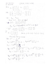
The practice exercise for mid term test | Môn Applied Linear Algebra - Trường Đại học Quốc tế, Đại học Quốc gia Thành phố Hồ Chí Minh
126 63 -
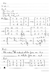
Matrix Echelon Forms and Inverses | Môn Applied Linear Algebra - Trường Đại học Quốc tế, Đại học Quốc gia Thành phố Hồ Chí Minh
103 52 -
Exercises: Matrices & Linear Equations (2021) | Môn Applied Linear Algebra - Trường Đại học Quốc tế, Đại học Quốc gia Thành phố Hồ Chí Minh
147 74 -

Final Exam Notes | Môn Applied Linear Algebra - Trường Đại học Quốc tế, Đại học Quốc gia Thành phố Hồ Chí Minh
120 60