Statistics Exercises: Full Questions and Solutions môn Thống kê trong kinh tế và kinh doanh | Trường Đại học Kinh tế Quốc dân
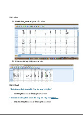
Shape: Slightly right-skewed due to high values (e.g. 2135)d) Observations: Most scores lie between 1200–1799, few high outlier. Tài liệu giúp bạn tham khảo, ôn tập và đạt kết quả cao. Mời đọc đón xem!
Môn: Thống kê trong kinh tế và kinh doanh 1.3 K tài liệu
Trường: Trường Đại học Kinh Tế Quốc Dân 8.2 K tài liệu
Tác giả:


Preview text:
Statistics Exercises: Full Questions and Solutions Chapter 2–3 Exercise 1
Data: 42, 66, 67, 71, 78, 62, 61, 76, 71, 67, 61, 64, 61, 54, 83, 63, 68, 69, 81, 53
a) Mean, Median, and Mode
Mean = (Sum of all values) / (Number of values) = (1306) / 20 = 65.3
Median: Sort data → 53, 54, 61, 61, 61, 62, 63, 64, 66, 67, 67, 68, 69, 71, 71, 76, 78, 81, 83
Middle two = 10th & 11th = 67 & 67 → Median = 67
Mode: Most frequent value = 61 (appears 3 times) → Mode = 61
b) Quartiles (Q1, Q3)
Q1 (25th percentile) = Average of 5th & 6th: (61 + 62)/2 = 61.5
Q3 (75th percentile) = Average of 15th & 16th: (71 + 76)/2 = 73.5 c) 90th Percentile
Position = 0.9 × 20 = 18 → 18th value = 81
→ Interpretation: 90% of jackets scored 81 or lower. Exercise 2
SAT Scores: 1665, 1490, 1680, 1420, 1485, 1585, 1275, 1525, 1560, 1440,
1755, 1990, 1650, 2135, 1355, 940, 1260, 1375, 1590, 1560, 1280, 1645,
1390, 1730, 1475, 1880, 1150, 1060, 1780, 1175
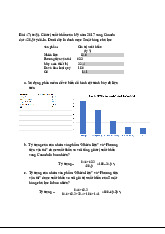
a) Frequency Distribution (Start = 800, Width = 200): Class Frequen Interval cy 800–999 1 1000–1199 3 Class Frequen Interval cy 1200–1399 7 1400–1599 8 1600–1799 7 1800–1999 3 2000–2199 1
b) Relative Frequency and Cumulative %: Interval Rel. Cum. Freq % 800–999 0.033 3.3% 1000– 1199 0.100 13.3% 1200– 1399 0.233 36.6% 1400– 1599 0.267 63.3% 1600– 1799 0.233 86.6% 1800– 1999 0.100 96.6% 2000– 2199 0.033 100%
c) Shape: Slightly right-skewed due to high values (e.g. 2135) d)
Observations: Most scores lie between 1200–1799, few high outliers
e) From Raw Data:
Mean = (Sum of values)/30 = 45,005 / 30 = 1500.2
Median = 15.5th value in sorted data = (1475+1485)/2 = 1480 Mode: 1560 (occurs twice)
f) From Frequency Distribution: Use midpoints × freq / total → approximate mean ≈ , 1497.3 median ≈ 1480
g) Comparison: Close estimates; frequency-based methods are approximations Exercise 3 City Price Sales ($) (cases) Bakersfield 34.99 501 Los Angeles 38.99 1425 Modesto 36.00 294 Oakland 33.59 882 Sacramento 40.99 715 San Diego 38.59 1088 San Francisco 39.59 1644 San Jose 37.99 819
Average price per case = Total revenue / Total quantity
=∑(Pi×Qi)∑Qi=289,417.418368≈34.59= \frac{\sum (P_i \times Q_i)}{\sum
Q_i} = \frac{289,417.41}{8368} ≈ \textbf{34.59} Exercise 4
Quarter-mile: 0.92, 0.98, 1.04, 0.90, 0.99
Mile: 4.52, 4.35, 4.60, 4.70, 4.50
Step 1: Compute Mean and SD for both
Q-mile: Mean = 0.966, SD ≈ 0.0523
Mile: Mean = 4.534, SD ≈ 0.1296
Step 2: CoefÏcient of Variation (CV) CV = SD / Mean × 100% Q-mile: ≈ 5.4% Mile: ≈ 2.86%
Conclusion: Despite the coach’s comment, mile runners were more consistent.
Statistics Exercises: Full Questions and Solutions Chapter 2–3 (... previous exercises ...) Exercise 5
Home Prices: 995.9, 48.8, 175.0, 263.5, 298.0, 218.0, 209.0, 628.3, 111.0,
212.9, 92.6, 2325.0, 958.0, 212.5
a) Median: Sort the data → 48.8, 92.6, 111.0, 175.0, 209.0, 212.5, 212.9,
218.0, 263.5, 298.0, 628.3, 958.0, 995.9, 2325.0
→ Middle = 7th & 8th → (212.9 + 218.0)/2 = 215.45
b) % Increase from $139.3 →
(215.45 – 139.3) / 139.3 × 100% ≈ 54.7%
c) Q1 = Median of lower 7 = 111.0 Q3 = Median of upper 7 = 958.0
IQR = Q3 – Q1 = 958.0 – 111.0 = 847.0 d) Boxplot:
Min = 48.8, Q1 = 111.0, Median = 215.45, Q3 = 958.0, Max = 2325.0 e) Outliers?
Lower Bound = Q1 – 1.5×IQR = –1159.5 → none
Upper Bound = Q3 + 1.5×IQR = 2228.5 → 2325 is an outlier
f) Mean = (Sum of all values)/14 = 7808 / 14 ≈ 557.7
→ Use median to avoid distortion from large outlier (2325) Exercise 6 Given: Mean = 547, SD = 100
a) P(X ≥ 647): Z = (647 – 547)/100 = 1 → P = 15.87%
b) P(X ≥ 747): Z = 2 → P = 2.28%
c) P(447 ≤ X ≤ 547): Z = –1 to 0 → P = 34.13%
d) P(347 ≤ X ≤ 647): Z = –2 to 1 → P = 81.85% Exercise 7
Mean = $3100, SD = $1200
a) Z = (2300 – 3100)/1200 = –0.667 → z = –0.67
b) Z = (4900 – 3100)/1200 = +1.5 c) Interpretation:
2300 is below average by ~0.67 SD
4900 is above average by 1.5 SD
d) Outlier? No (not beyond ±3 SD)
e) $13,000 → Z = (13000 – 3100)/1200 = 8.25 → Yes, it's a strong outlier Exercise 8
Data: 55, 56, 44, 43, 44, 56, 60, 62, 57, 45, 36, 38, 50, 69, 65
a) Mean = Sum/15 = 804 / 15 = 53.6 Median = 50
b) Q1 = 44, Q3 = 60 → IQR = 16 c) Range = 69 – 36 = 33 IQR = 60 – 44 = 16 d) Variance:
Find (x – mean)² for each, sum = 1536.4
Var = 1536.4 / 14 = 109.7 → SD ≈ 10.47
e) Boxplot values: Min = 36, Q1 = 44, Med = 50, Q3 = 60, Max = 69 → No outlier
f) Walmart goal ≈ 50% layoff. Mean = 53.6% → Likely not meeting goal Exercise 9
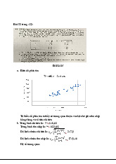
Speed vs MPG – [Data not included]
a) Scatter diagram → visual upward/downward trend
b) Interpret correlation visually: e.g., negative → as speed ↑, MPG ↓
c) Covariance = measure of joint variability
d) Correlation coefÏcient (r): r = cov(X,Y) / (SD_X × SD_Y)
If r ≈ –1 → strong negative
(If you want, I’ll continue with Chapter 4 next. Ready?)
Tài liệu liên quan:
-
Ôn tập nhóm Bài Tập Hồi Quy | Thống kê trong kinh tế và kinh doanh | Trường Đại học Kinh tế Quốc dân
17 9 -
Thống Kê Xuất Nhập Khẩu và Giá Trị Hàng Hóa | Thống kê trong kinh tế và kinh doanh | Trường Đại học Kinh tế Quốc dân
20 10 -
Bài Tập Thống Kê Kinh Doanh | Thống kê trong kinh tế và kinh doanh | Trường Đại học Kinh tế Quốc dân
17 9 -
Bài tập Phân tích sự sụp đổ của Thomas Cook trong ngành du lịch | Thống kê trong kinh tế và kinh doanh | Trường Đại học Kinh tế Quốc dân
18 9 -
Thực Hành C1: Phân Tích Dữ Liệu Bất Động Sản Trên SPSS | Thống kê trong kinh tế và kinh doanh | Trường Đại học Kinh tế Quốc dân
13 7