Sticky-Price Monetary Models of Exchange Rates: A Study on 2009 | Tài chính quốc tế | Trường Học Viện nông nghiệp Việt Nam
The asset market model of exchange rate determination underwent considerable development during the first decade following the floating of major currencies (1973–83). This is because simple models were found to explain the behavior of the post-Bretton Woods floating exchange rates poorly and also because the availability of a larger set of data on the floating period provided the opportunity to carry out more empirical work. 1 The very high volatility of the real exchange rates of major currencies in the late 1970s casts doubt on PPP and inspired the development of further versions of the monetary model, including the sticky-price monetary model of Dornbusch (1976c). Tài liệu được sưu tầm và soạn thảo dưới dạng file PDF để gửi tới các bạn cùng tham khảo, ôn tập đầy đủ kiến thức, chuẩn bị cho các buổi học thật tốt. Mời bạn đọc đón xem!
Môn: Tài chính quốc tế (hvnn) 130 tài liệu
Trường: Học viện Nông nghiệp Việt Nam 2.4 K tài liệu
Tác giả:


Preview text:
CHAPTER 6
Other Sticky-Price Monetary Models of Exchange Rates fic.com 6.1. Introduction
The asset market model of exchange rate determination underwent consid-
erable development during the first decade following the floating of major
currencies (1973–83). This is because simple models were found to explain
the behavior of the post-Bretton Woods floating exchange rates poorly and
also because the availability of a larger set of data on the floating period
provided the opportunity to carry out more empirical work.1 The very high
volatility of the real exchange rates of major currencies in the late 1970s
casts doubt on PPP and inspired the development of further versions of the
monetary model, including the sticky-price monetary model of Dornbusch (1976c).
During the late 1970s and early 1980s, a wide range of overshooting
models were constructed to explain new stylized facts or events asso-
ciated with the floating rate period. Included in these models are the real
interest differential sticky-price monetary model of Frankel (1979b), the
stock-flow model of Driskell (1981), and the equilibrium real exchange
by UNIVERSITY OF MELBOURNE on 01/13/17. For personal use only.
rate sticky-price model of Hooper and Morton (1982). Yet, the empirical
validity of these variants of the sticky-price model has proven to be more
The Theory and Empirics of Exchange Rates Downloaded from www.worldscienti elusive.
In the simple flexible-price model, the exchange rate is determined by
stock equilibrium in money markets, which is achieved very quickly (if not
instantaneously) through continuous adjustment of prices in the goods and
asset markets, while complete neutrality of monetary policy is maintained
1For a detailed analysis of the development of the asset-market model of exchange rate
determination and the events of the current floating rate period leading to modifications and
extensions in the theory, see Dornbusch (1980b) and Shafer et al. (1983). 186
Other Sticky-Price Monetary Models of Exchange Rates 187
on a continuous basis. This model appears to fit the data fairly well for the
first four years of flexible exchange rates (1973–76), as indicated by the
evidence presented by Hodrick (1978) and Bilson (1978a). In subsequent
studies (which tested the model for a slightly larger set of data incorporating
the period 1977–78), the performance of this model deteriorated severely.
This led to considerable concern with respect to a reconciliation of the
simple monetary model with the observed large fluctuations in exchange rates.
By late 1975, little correspondence was found between exchange rates
and prices in many major industrial countries (at least in the short run) and it fic.com
was also found that changes over time in the real exchange rates were much
larger than those under fixed exchange rates. Inflation rates diverged widely
between these countries, while exchange rates showed some tendency to
change over time to contain deviation from purchasing power parity. Never-
theless, most fluctuations in nominal exchange rates over the period March
1973 to September 1975 were reflected in the movements of real exchange
rates. It was against this backdrop that Dornbusch (1976c) developed the
sticky-price version of the monetary model. This model is consistent with
several stylized facts that do not fit well with the flexible-price model. Not
only does it rationalize deviations from purchasing power parity in the short
run, it also provides an explanation for periods when a rising nominal interest
rate is associated with a strong currency. In the flexible-price model, a rise in
the nominal interest rate is always associated with an increase in the inflation
rate and more rapid depreciation (or less rapid appreciation) of the currency.
In the sticky-price model, a persistently higher level of the interest rate
reflects higher inflation, which makes it associated with a weaker currency.
But an increase in the interest rate and declining inflationary expectations
may be produced by a shift to tight monetary policy, leading to currency
by UNIVERSITY OF MELBOURNE on 01/13/17. For personal use only. appreciation.
The sticky-price model suggests that the relation between changes in
The Theory and Empirics of Exchange Rates Downloaded from www.worldscienti
the exchange rate and monetary aggregates is not simple even when mon-
etary disturbances are the underlying cause. Expectations concerning future
levels of the money supply are more important than the current levels of
the money supply, which means that poor correlation between contempora-
neous changes in monetary aggregates and exchange rates is explainable. It
must be noted, however, that evidence on the sticky-price model is not very
much different from the evidence on the flexible-price model, particularly
during the first 4 years of the current flexible exchange rate period. This is 188
The Theory and Empirics of Exchange Rates
why the empirical basis for a choice between the flexible- and sticky-price
versions of the monetary model is not clear.
Frankel (1979b) modified the Dornbusch (1976c) sticky-price model by
allowing a role for differences in secular inflation rates, hence including the
real interest differential as an additional explanatory variable. He argues
that changes in long-term nominal interest rates are a measure of changes
in inflation expectations. According to this view, only short-term interest
rates are viewed as moving somewhat independently of inflation. Therefore,
Frankel includes the long-term interest rate differential in the exchange
rate equation either because long-term interest rates measure the cost of fic.com
holding money or because they are considered as a proxy for the anticipated
inflation differential. In either view, a rise in the domestic long-term interest
differential leads to a reduction in real money demand and thus to higher
prices and currency depreciation.
Frankel (1979b) tested the real interest differential model for the
mark/dollar rate from July 1974 to February 1978 and found evidence
that clearly supported the model against the flexible- and the sticky-price
versions of the monetary model. However, subsequent attempts by Dorn-
busch (1980b), Haynes and Stone (1981), and Frankel (1981) to explain
movements in the mark/dollar exchange rate after February 1978 were
unsuccessful, showing insignificant coefficients and a “reversed sign” on
the relative money coefficient. An important phenomenon that was not
directly explainable by the sticky-price models of Dornbusch (1976c) and
Frankel (1979b) was the large and growing deficit in the U.S. current
account and the surpluses of Germany and Japan. Many observers began
to view the 1978–79 slide of the U.S. dollar as primarily an adjustment
to this large and growing deficit in the U.S. current account and sur-
pluses in Germany and Japan.2 In early 1975, a surplus arose in the U.S.
by UNIVERSITY OF MELBOURNE on 01/13/17. For personal use only.
current account as the sharp U.S. recession reduced imports. But with the
recovery of the economy and the dollar, the current account began to decline
The Theory and Empirics of Exchange Rates Downloaded from www.worldscienti
rapidly. This phenomenon induced many economists to turn to models
that assign a role to the current account in the process of exchange rate determination.
One popular model that gives a role to the current account in exchange
rate determination is the equilibrium real exchange rate model of Hooper
2Note that current account imbalances have been larger and more volatile during the floating
period than they had been during the Bretton Woods period.
Other Sticky-Price Monetary Models of Exchange Rates 189
and Morton (1982).3 They modified the Dornbusch–Frankel sticky-price
models by allowing large and sustained changes in real exchange rates,
which are related to movements in the current account (both through
changes in expectations about the long-run real exchange rate and through
changes in the risk premium). In particular, they show that the equilibrium
real exchange rate (defined as the rate that is consistent with the long-
run current account balance) can be expressed as a function of the initial
equilibrium rate and the cumulative sum of past non-transitory unexpected
changes in the current account. Hooper and Morton (1982) tested this fic.com
model empirically for the dollar’s weighted average exchange rate (against
the currencies of Belgium, Canada, France, Germany, Italy, Japan, the
Netherlands, Sweden, and the U.K.) over the flexible rate period of 1973–
78. They obtained results indicating that the current account affected the
exchange rate predominantly through its impact on expectations about the
long-run equilibrium real exchange rate. According to them, these results
are a reflection of the period extending between the end of 1976 and the end
of 1978, when the dollar depreciated steadily in real terms as the U.S. ran
a series of large current account deficits.
Frankel (1982a) adopts an alternative strategy to take account of the
role of the current account in the Dornbusch–Frankel sticky-price model.
He modifies money market conditions (stated in terms of the domestic and
foreign money demand functions and the exchange rate equation) by adding
relative wealth as an additional explanatory variable. The logic underlying
this formulation goes as follows. A foreign current account surplus repre-
sents a redistribution of wealth from domestic residents to foreign residents,
simultaneously raising foreign money demand, lowering domestic money
demand, and raising the exchange rate.
by UNIVERSITY OF MELBOURNE on 01/13/17. For personal use only.
3Other models that give a specific role to the current account in the determination of exchange
rates are the portfolio balance models that were originated by Branson (1976), Girton and
The Theory and Empirics of Exchange Rates Downloaded from www.worldscienti
Henderson (1976), Kouri et al. (1978), Dooley and Isard (1979, 1982, 1983), Dornbusch
(1980a), and Allen and Kenen (1980). Within the theoretical framework of slowly adjusting
commodity prices, an alternative to Dornbusch’s view of exchange rate dynamics, the
portfolio balance models emphasize stock-flow interaction and relative-price trade-balance
effects. In contrast to the monetary models, domestic and foreign bonds are assumed to be
imperfect substitutes. Thus, an increase in a country’s wealth (which is caused by a surplus
in its current account) leads to an increase in the demand for domestic bonds and hence
appreciation of the domestic currency. For a detailed discussion of portfolio balance models, see Chapter 8. 190
The Theory and Empirics of Exchange Rates
Another interesting variant of the sticky-price model (developed in
the context of the portfolio balance effect) is due to Driskell (1981). He
developed a stock-flow model that generalizes the Dornbusch (1976c)
model, permitting imperfect substitutability between domestic and foreign
assets and allowing trade flows to affect financial markets through the
balance of payments. In this model, portfolio allocation may affect the
exchange rate. He derives a reduced form exchange rate equation by
replacing the uncovered interest parity condition in Dornbusch’s (1976c)
framework with a balance of payments equation. fic.com
6.2. The Real Interest Differential Monetary Model
Frankel (1979b) argues that the flexible-price monetary model (what he
called the “Chicago theory of exchange rate”) and the sticky-price mon-
etary model (what he called the “Keynesian theory of exchange rate”) have
conflicting implications, particularly for the relation between exchange and
interest rates. In the following two subsections, the real interest differential model is described.
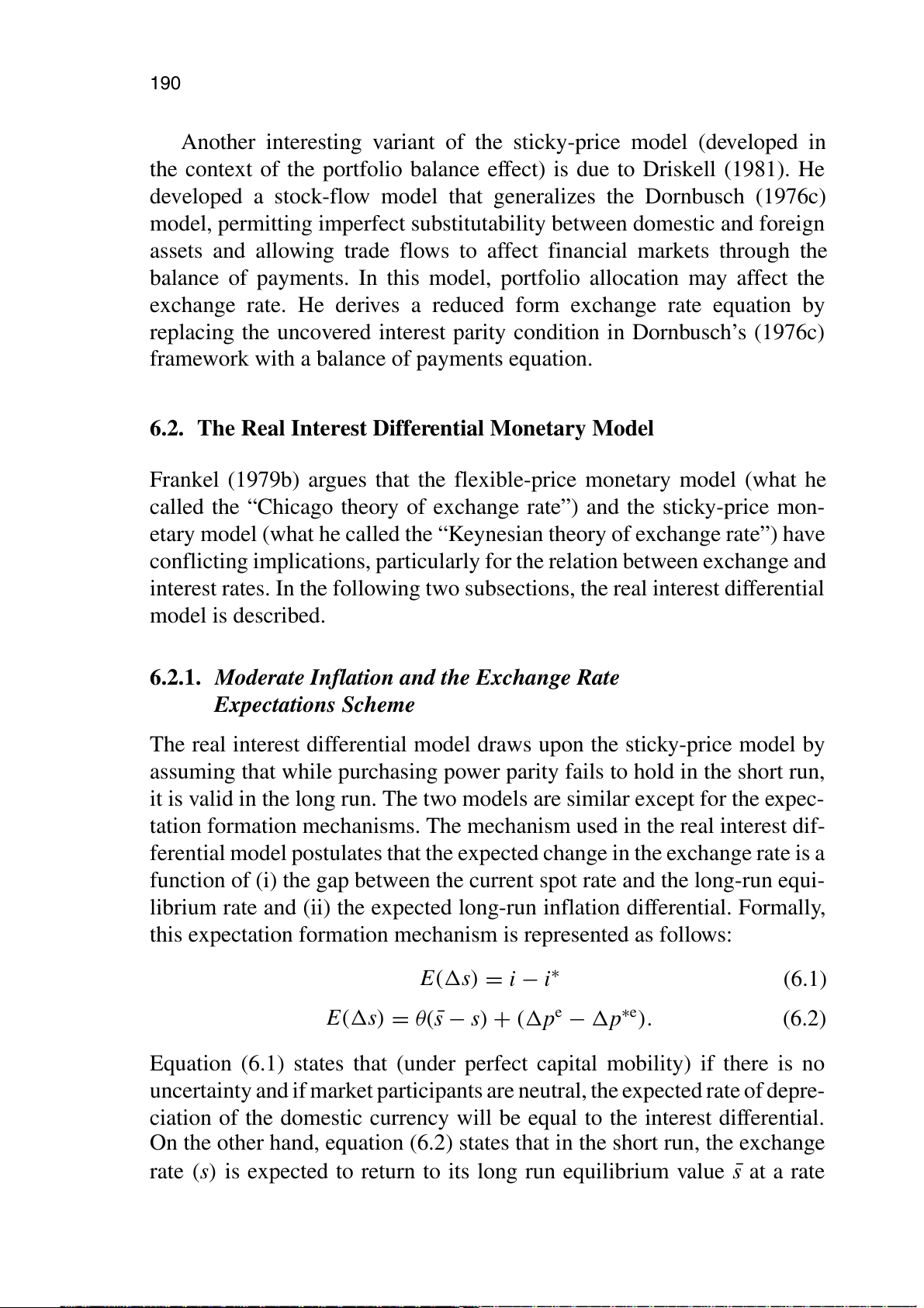
6.2.1. Moderate Inflation and the Exchange Rate
Expectations Scheme
The real interest differential model draws upon the sticky-price model by
assuming that while purchasing power parity fails to hold in the short run,
it is valid in the long run. The two models are similar except for the expec-
tation formation mechanisms. The mechanism used in the real interest dif-
ferential model postulates that the expected change in the exchange rate is a
function of (i) the gap between the current spot rate and the long-run equi-
by UNIVERSITY OF MELBOURNE on 01/13/17. For personal use only.
librium rate and (ii) the expected long-run inflation differential. Formally,
this expectation formation mechanism is represented as follows:
The Theory and Empirics of Exchange Rates Downloaded from www.worldscienti E(s) = i − i∗ (6.1) E(s) = θ( ¯
s − s) + (pe − p∗e). (6.2)
Equation (6.1) states that (under perfect capital mobility) if there is no
uncertainty and if market participants are neutral, the expected rate of depre-
ciation of the domestic currency will be equal to the interest differential.
On the other hand, equation (6.2) states that in the short run, the exchange
rate (s) is expected to return to its long run equilibrium value ¯ s at a rate
Other Sticky-Price Monetary Models of Exchange Rates 191
that is proportional to the current gap. In the long run (when ¯ s = s), the
exchange rate is expected to change at a rate that is equal to the long-run
inflation differential (pe − p∗e), which is equal to the expected long-run
relative monetary growth rate that is known to the public. By combining
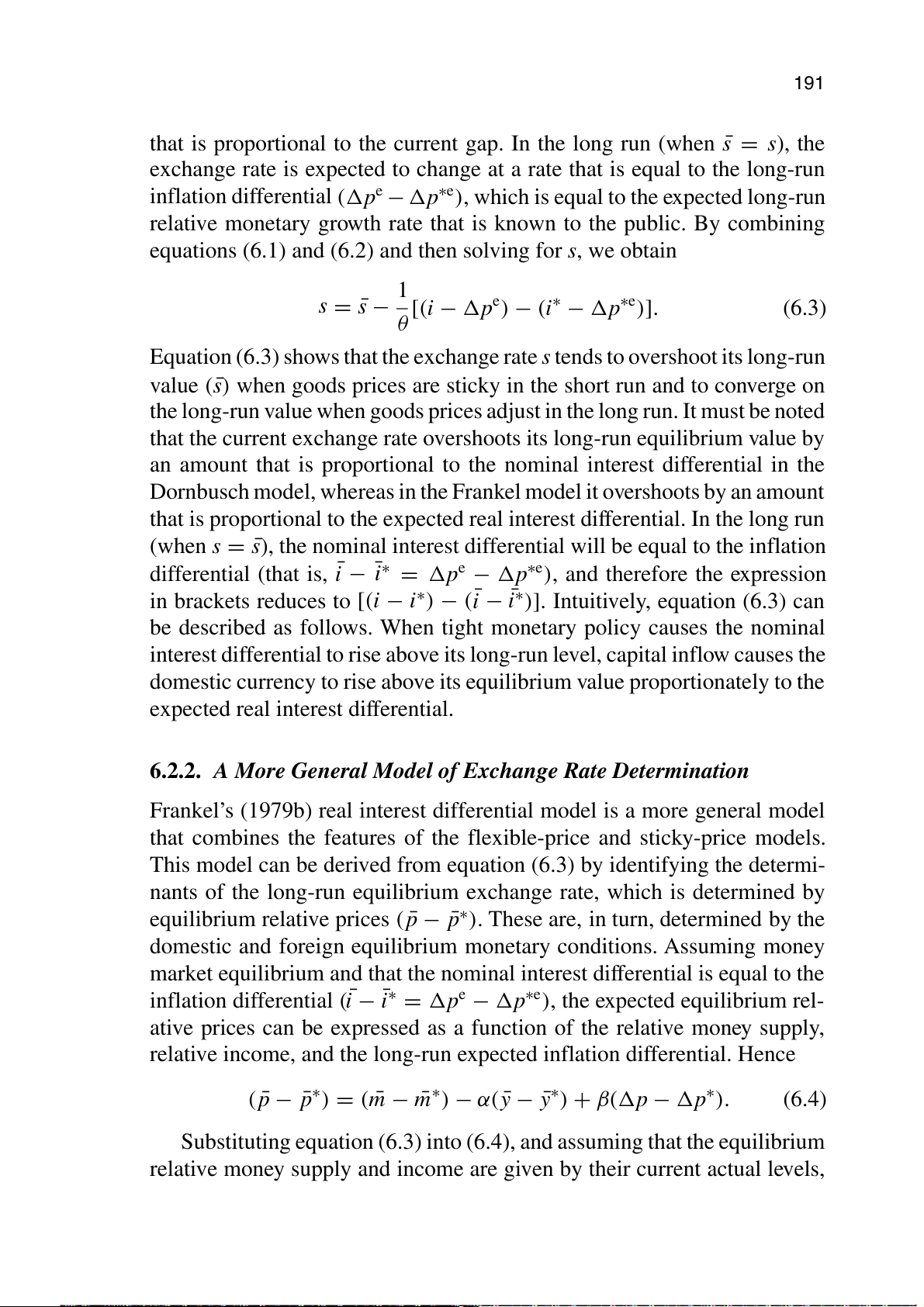
equations (6.1) and (6.2) and then solving for s, we obtain 1 s = ¯ s −
[(i − pe) − (i∗ − p∗e)]. (6.3) θ
Equation (6.3) shows that the exchange rate s tends to overshoot its long-run value ( ¯
s) when goods prices are sticky in the short run and to converge on fic.com
the long-run value when goods prices adjust in the long run. It must be noted
that the current exchange rate overshoots its long-run equilibrium value by
an amount that is proportional to the nominal interest differential in the
Dornbusch model, whereas in the Frankel model it overshoots by an amount
that is proportional to the expected real interest differential. In the long run (when s = ¯
s), the nominal interest differential will be equal to the inflation
differential (that is, ¯i − ¯i∗ = pe − p∗e), and therefore the expression
in brackets reduces to [(i − i∗) − ( ¯i − ¯
i∗)]. Intuitively, equation (6.3) can
be described as follows. When tight monetary policy causes the nominal
interest differential to rise above its long-run level, capital inflow causes the
domestic currency to rise above its equilibrium value proportionately to the
expected real interest differential.
6.2.2. A More General Model of Exchange Rate Determination
Frankel’s (1979b) real interest differential model is a more general model
that combines the features of the flexible-price and sticky-price models.
This model can be derived from equation (6.3) by identifying the determi-
by UNIVERSITY OF MELBOURNE on 01/13/17. For personal use only.
nants of the long-run equilibrium exchange rate, which is determined by
equilibrium relative prices ( ¯ p − ¯
p∗). These are, in turn, determined by the
The Theory and Empirics of Exchange Rates Downloaded from www.worldscienti
domestic and foreign equilibrium monetary conditions. Assuming money
market equilibrium and that the nominal interest differential is equal to the inflation differential ( ¯
i − ¯i∗ = pe − p∗e), the expected equilibrium rel-
ative prices can be expressed as a function of the relative money supply,
relative income, and the long-run expected inflation differential. Hence ( ¯ p − ¯ p∗) = ( ¯ m − ¯ m∗) − α( ¯ y − ¯ y∗) + β(p − p∗). (6.4)
Substituting equation (6.3) into (6.4), and assuming that the equilibrium
relative money supply and income are given by their current actual levels, 192
The Theory and Empirics of Exchange Rates
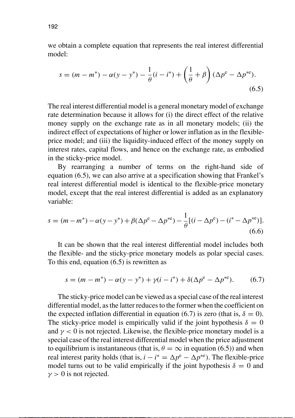
we obtain a complete equation that represents the real interest differential model: 1 1
s = (m − m∗) − α(y − y∗) − (i − i∗) + + β (pe − p∗e). θ θ (6.5)
The real interest differential model is a general monetary model of exchange
rate determination because it allows for (i) the direct effect of the relative
money supply on the exchange rate as in all monetary models; (ii) the fic.com
indirect effect of expectations of higher or lower inflation as in the flexible-
price model; and (iii) the liquidity-induced effect of the money supply on
interest rates, capital flows, and hence on the exchange rate, as embodied in the sticky-price model.
By rearranging a number of terms on the right-hand side of
equation (6.5), we can also arrive at a specification showing that Frankel’s
real interest differential model is identical to the flexible-price monetary
model, except that the real interest differential is added as an explanatory variable: 1
s = (m − m∗) − α(y − y∗) + β(pe − p∗e) − [(i − pe) − (i∗ − p∗e)]. θ (6.6)
It can be shown that the real interest differential model includes both
the flexible- and the sticky-price monetary models as polar special cases.
To this end, equation (6.5) is rewritten as
s = (m − m∗) − α(y − y∗) + γ(i − i∗) + δ(pe − p∗e). (6.7)
by UNIVERSITY OF MELBOURNE on 01/13/17. For personal use only.
The sticky-price model can be viewed as a special case of the real interest
The Theory and Empirics of Exchange Rates Downloaded from www.worldscienti
differential model, as the latter reduces to the former when the coefficient on
the expected inflation differential in equation (6.7) is zero (that is, δ = 0).
The sticky-price model is empirically valid if the joint hypothesis δ = 0
and γ < 0 is not rejected. Likewise, the flexible-price monetary model is a
special case of the real interest differential model when the price adjustment
to equilibrium is instantaneous (that is, θ = ∞ in equation (6.5)) and when
real interest parity holds (that is, i − i∗ = pe − p∗e). The flexible-price
model turns out to be valid empirically if the joint hypothesis δ = 0 and γ > 0 is not rejected.
Other Sticky-Price Monetary Models of Exchange Rates 193
6.3. Driskell’s Generalized Stock-Flow Sticky-Price Model
Driskell (1981) argues that two striking implications follow from the
Dornbusch (1976c) model. First, in response to a change in relative money
supplies, the exchange rate may change immediately by more than the
long-run equilibrium value determined by purchasing power parity. In other
words, the exchange rate may overshoot its long-run purchasing power
parity value in the short run. Second, following this initial overshooting, the
exchange rate approaches monotonically its long-run equilibrium value. He
argues that both of these implications result from the key assumptions of fic.com
sticky prices and perfect capital mobility. Following the work of Branson
(1976), Niehans (1977), and Henderson (1980) (who have developed an
alternative view of exchange rate dynamics emphasizing stock-flow inter-
actions and relative-price trade-balance effects), Driskell (1981) developed
a generalized stock-flow variant of the Dornbusch model, leading to con-
trasting results of short-run undershooting and non-monotonic exchange
rate and price level adjustments.
Driskell (1981) generalizes the Dornbusch (1976c) overshooting model
to develop two structural models (what he calls the Dornbusch model in
discrete time and a stock-flow model) by allowing imperfect substitutability
between domestic and foreign assets. He argues that both of these structural
models impose a priori constraints on the reduced-form parameters and
thus can (in principle) be rejected by the data.
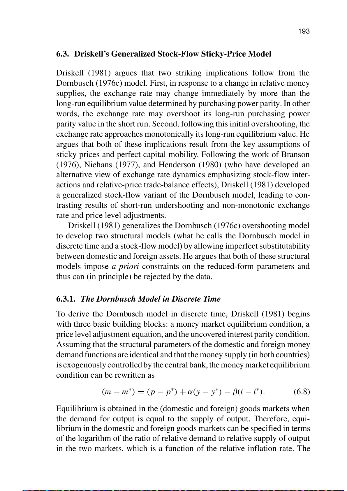
6.3.1. The Dornbusch Model in Discrete Time
To derive the Dornbusch model in discrete time, Driskell (1981) begins
with three basic building blocks: a money market equilibrium condition, a
by UNIVERSITY OF MELBOURNE on 01/13/17. For personal use only.
price level adjustment equation, and the uncovered interest parity condition.
Assuming that the structural parameters of the domestic and foreign money
demand functions are identical and that the money supply (in both countries)
The Theory and Empirics of Exchange Rates Downloaded from www.worldscienti
is exogenously controlled by the central bank, the money market equilibrium condition can be rewritten as
(m − m∗) = (p − p∗) + α(y − y∗) − β(i − i∗). (6.8)
Equilibrium is obtained in the (domestic and foreign) goods markets when
the demand for output is equal to the supply of output. Therefore, equi-
librium in the domestic and foreign goods markets can be specified in terms
of the logarithm of the ratio of relative demand to relative supply of output
in the two markets, which is a function of the relative inflation rate. The 194
The Theory and Empirics of Exchange Rates
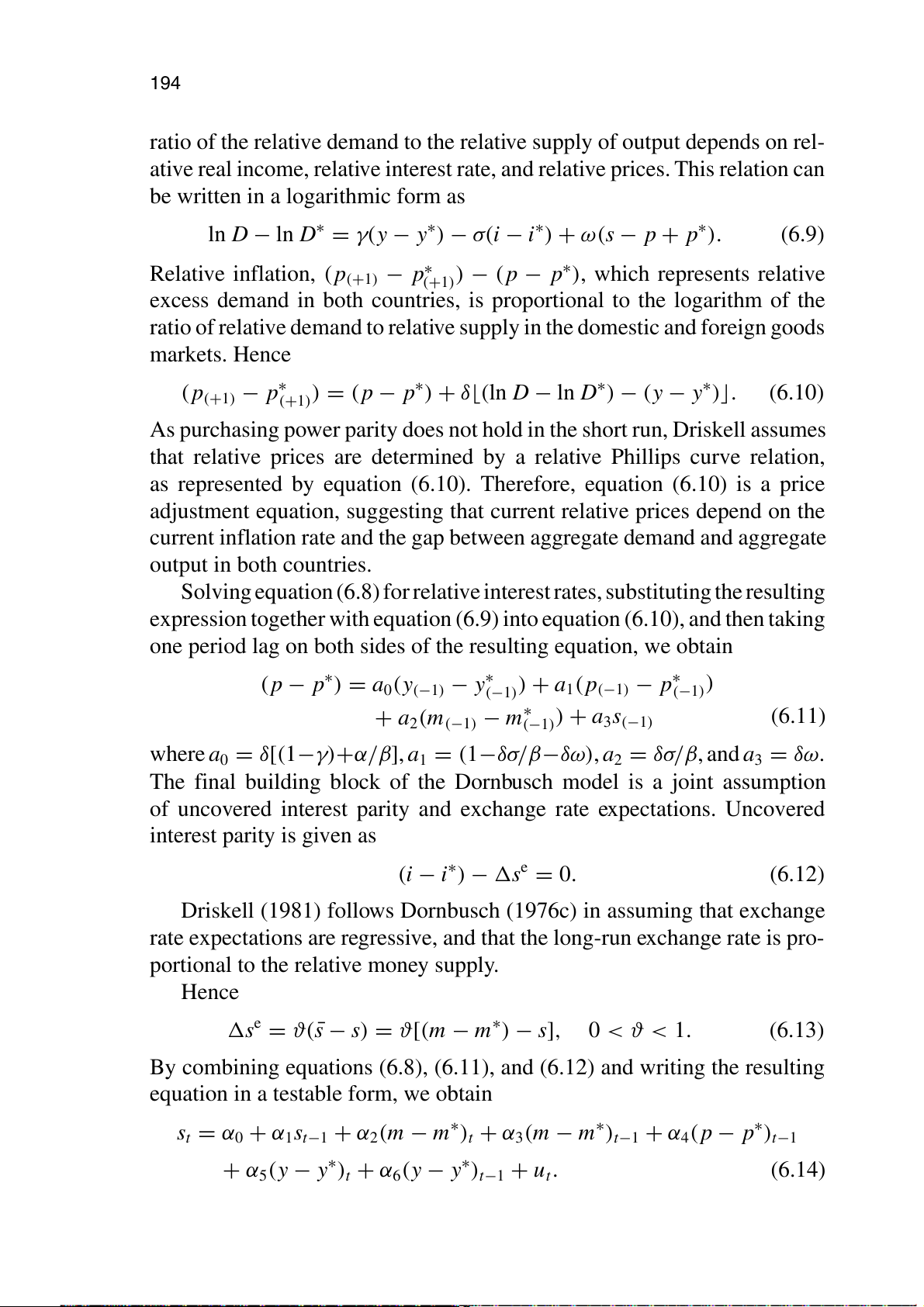
ratio of the relative demand to the relative supply of output depends on rel-
ative real income, relative interest rate, and relative prices. This relation can
be written in a logarithmic form as
ln D − ln D∗ = γ(y − y∗) − σ(i − i∗) + ω(s − p + p∗). (6.9)
Relative inflation, (p(+1) − p∗
) − (p − p∗), which represents relative (+1)
excess demand in both countries, is proportional to the logarithm of the
ratio of relative demand to relative supply in the domestic and foreign goods markets. Hence fic.com (p(+1) − p∗
) = (p − p∗) + δ(ln D − ln D∗) − (y − y∗). (6.10) (+1)
As purchasing power parity does not hold in the short run, Driskell assumes
that relative prices are determined by a relative Phillips curve relation,
as represented by equation (6.10). Therefore, equation (6.10) is a price
adjustment equation, suggesting that current relative prices depend on the
current inflation rate and the gap between aggregate demand and aggregate output in both countries.
Solving equation (6.8) for relative interest rates, substituting the resulting
expression together with equation (6.9) into equation (6.10), and then taking
one period lag on both sides of the resulting equation, we obtain
(p − p∗) = a0(y(−1) − y∗ ) + a ) (−1) 1(p(−1) − p∗ (−1) + a ∗ 2(m(−1) − m ) + a (−1) 3s(−1) (6.11)
where a0 = δ[(1−γ)+α/β], a1 = (1−δσ/β−δω), a2 = δσ/β, and a3 = δω.
The final building block of the Dornbusch model is a joint assumption
of uncovered interest parity and exchange rate expectations. Uncovered interest parity is given as (i − i∗) − se = 0. (6.12)
by UNIVERSITY OF MELBOURNE on 01/13/17. For personal use only.
Driskell (1981) follows Dornbusch (1976c) in assuming that exchange
rate expectations are regressive, and that the long-run exchange rate is pro-
The Theory and Empirics of Exchange Rates Downloaded from www.worldscienti
portional to the relative money supply. Hence se = ϑ( ¯
s − s) = ϑ[(m − m∗) − s], 0 < ϑ < 1. (6.13)
By combining equations (6.8), (6.11), and (6.12) and writing the resulting
equation in a testable form, we obtain s ∗
t = α0 + α1st−1 + α2(m − m∗)t + α3(m − m )t−1 + α4(p − p∗)t−1
+ α5(y − y∗)t + α6(y − y∗)t−1 + ut. (6.14)
Other Sticky-Price Monetary Models of Exchange Rates 195
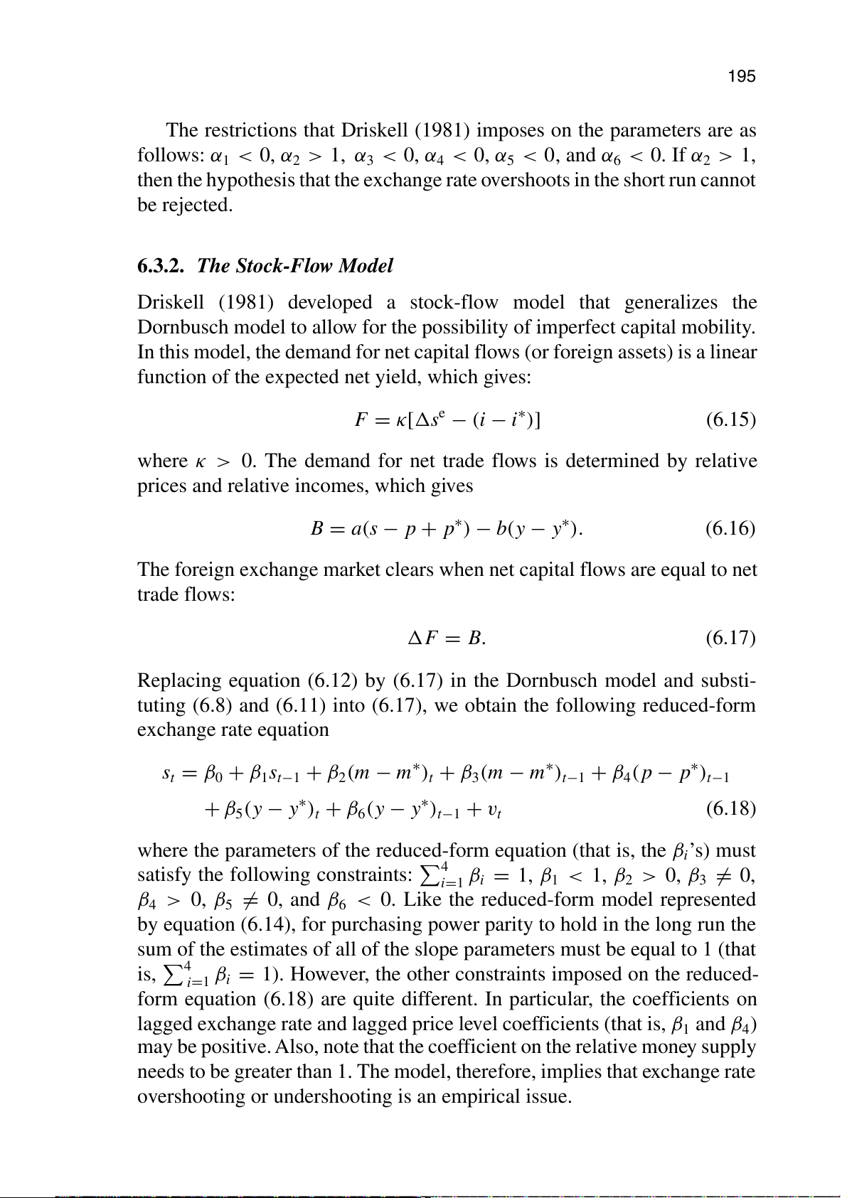
The restrictions that Driskell (1981) imposes on the parameters are as
follows: α1 < 0, α2 > 1, α3 < 0, α4 < 0, α5 < 0, and α6 < 0. If α2 > 1,
then the hypothesis that the exchange rate overshoots in the short run cannot be rejected.
6.3.2. The Stock-Flow Model
Driskell (1981) developed a stock-flow model that generalizes the
Dornbusch model to allow for the possibility of imperfect capital mobility.
In this model, the demand for net capital flows (or foreign assets) is a linear fic.com
function of the expected net yield, which gives: F = κ[se − (i − i∗)] (6.15)
where κ > 0. The demand for net trade flows is determined by relative
prices and relative incomes, which gives
B = a(s − p + p∗) − b(y − y∗). (6.16)
The foreign exchange market clears when net capital flows are equal to net trade flows: F = B. (6.17)
Replacing equation (6.12) by (6.17) in the Dornbusch model and substi-
tuting (6.8) and (6.11) into (6.17), we obtain the following reduced-form exchange rate equation s ∗ ∗
t = β0 + β1st−1 + β2(m − m∗)t + β3(m − m )t−1 + β4(p − p )t−1
+ β5(y − y∗)t + β6(y − y∗)t−1 + vt (6.18)
by UNIVERSITY OF MELBOURNE on 01/13/17. For personal use only.
where the parameters of the reduced-form equation (that is, the βi’s) must
The Theory and Empirics of Exchange Rates Downloaded from www.worldscienti
satisfy the following constraints: 4 β β β i=1 i = 1, 1 < 1, 2 > 0, β3 = 0,
β4 > 0, β5 = 0, and β6 < 0. Like the reduced-form model represented
by equation (6.14), for purchasing power parity to hold in the long run the
sum of the estimates of all of the slope parameters must be equal to 1 (that is, 4 β i=1
i = 1). However, the other constraints imposed on the reduced-
form equation (6.18) are quite different. In particular, the coefficients on
lagged exchange rate and lagged price level coefficients (that is, β1 and β4)
may be positive. Also, note that the coefficient on the relative money supply
needs to be greater than 1. The model, therefore, implies that exchange rate
overshooting or undershooting is an empirical issue. 196
The Theory and Empirics of Exchange Rates
Driskell’s model yields predictions that are clearly different from those
of the Dornbusch (1976c) and Frankel (1979b) models. The long-run
neutrality of money still holds but exchange rate overshooting is no longer
essential. With perfect substitutability between domestic and foreign assets,
α2 in the model represented by equation (6.14) would exceed one as a result
of exchange rate overshooting. With imperfect substitutability, however, the
initial response of the exchange rate to a monetary shock may be to over-
shoot or undershoot its long-run value. fic.com
6.4. The Equilibrium Real Exchange Rate Monetary Model
Hooper and Morton (1982) argue that the most serious deficiency of the
monetary model is that it neglects changes in external trade imbalances and
the impact these changes have on the exchange rate. The current account,
however, does not affect the exchange rate directly but only indirectly
through its impact on exchange rate expectations. Hooper and Morton
developed the equilibrium real exchange rate model that draws from mon-
etary and portfolio balance models. This model allows explicitly for the
short-run impact on the exchange rate of both the current account and
imperfect substitutability of assets.
The Hooper–Morton model is, in fact, an extension of the Dornbusch–
Frankel model that allows for large and sustained changes in real exchange
rates. The Dornbusch–Frankel model is modified to allow for shifts in
the long-run equilibrium real exchange rate and the existence of risk
premium. The Hooper–Morton model assumes that there is an equilibrium
real exchange rate that is expected to maintain current account equilibrium
in the long run. But at any point time, the equilibrium real exchange rate
is determined by the cumulative sum of past and present current account
by UNIVERSITY OF MELBOURNE on 01/13/17. For personal use only.
balances. Thus, an unexpected permanent rise in the cumulative current
account surplus will require an upward adjustment in the equilibrium long-
The Theory and Empirics of Exchange Rates Downloaded from www.worldscienti
run real exchange rate if the current account is to be eventually balanced.
This upward adjustment in the equilibrium long-run real exchange rate in
turn affects the equilibrium long-run nominal exchange rate through the
purchasing power parity channel.
6.4.1. The Expectation Mechanism and Exchange
Rate Determination
Hooper and Morton begin by arguing that unexpected changes in the current
account provide information about shifts in the underlying determinants that
Other Sticky-Price Monetary Models of Exchange Rates 197
make it necessary for offsetting shifts in the real exchange rate to maintain
current account equilibrium in the long run. An important point is that it
is only the unexpected component of the current account that affects the
exchange rate (the expected component is already taken into account by
the foreign exchange market). Therefore, the release by the government of
unexpected figures on the trade balance or current account appears to have
large immediate announcement effects on the exchange rate.
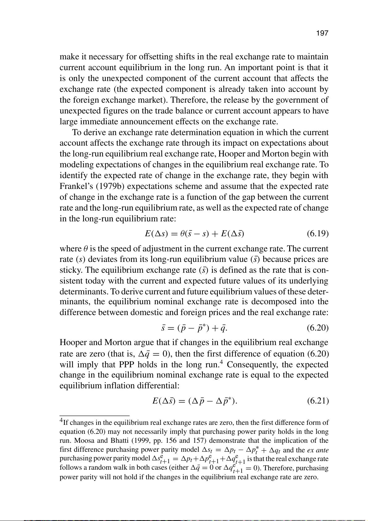
To derive an exchange rate determination equation in which the current
account affects the exchange rate through its impact on expectations about
the long-run equilibrium real exchange rate, Hooper and Morton begin with fic.com
modeling expectations of changes in the equilibrium real exchange rate. To
identify the expected rate of change in the exchange rate, they begin with
Frankel’s (1979b) expectations scheme and assume that the expected rate
of change in the exchange rate is a function of the gap between the current
rate and the long-run equilibrium rate, as well as the expected rate of change
in the long-run equilibrium rate: E(s) = θ( ¯ s − s) + E( ¯ s) (6.19)
where θ is the speed of adjustment in the current exchange rate. The current
rate (s) deviates from its long-run equilibrium value ( ¯ s) because prices are
sticky. The equilibrium exchange rate ( ¯
s) is defined as the rate that is con-
sistent today with the current and expected future values of its underlying
determinants. To derive current and future equilibrium values of these deter-
minants, the equilibrium nominal exchange rate is decomposed into the
difference between domestic and foreign prices and the real exchange rate: ¯s = ( ¯ p − ¯ p∗) + ¯ q. (6.20)
Hooper and Morton argue that if changes in the equilibrium real exchange rate are zero (that is, ¯
q = 0), then the first difference of equation (6.20)
by UNIVERSITY OF MELBOURNE on 01/13/17. For personal use only.
will imply that PPP holds in the long run.4 Consequently, the expected
change in the equilibrium nominal exchange rate is equal to the expected
The Theory and Empirics of Exchange Rates Downloaded from www.worldscienti
equilibrium inflation differential: E( ¯ s) = ( ¯ p − ¯ p∗). (6.21)
4If changes in the equilibrium real exchange rates are zero, then the first difference form of
equation (6.20) may not necessarily imply that purchasing power parity holds in the long
run. Moosa and Bhatti (1999, pp. 156 and 157) demonstrate that the implication of the
first difference purchasing power parity model s ∗
t = pt − pt + qt and the ex ante
purchasing power parity model se = p e t +p +qe t+1 t+1 is that the real exchange rate t+1
follows a random walk in both cases (either ¯ q = 0 or qe = 0). Therefore, purchasing t+1
power parity will not hold if the changes in the equilibrium real exchange rate are zero. 198
The Theory and Empirics of Exchange Rates
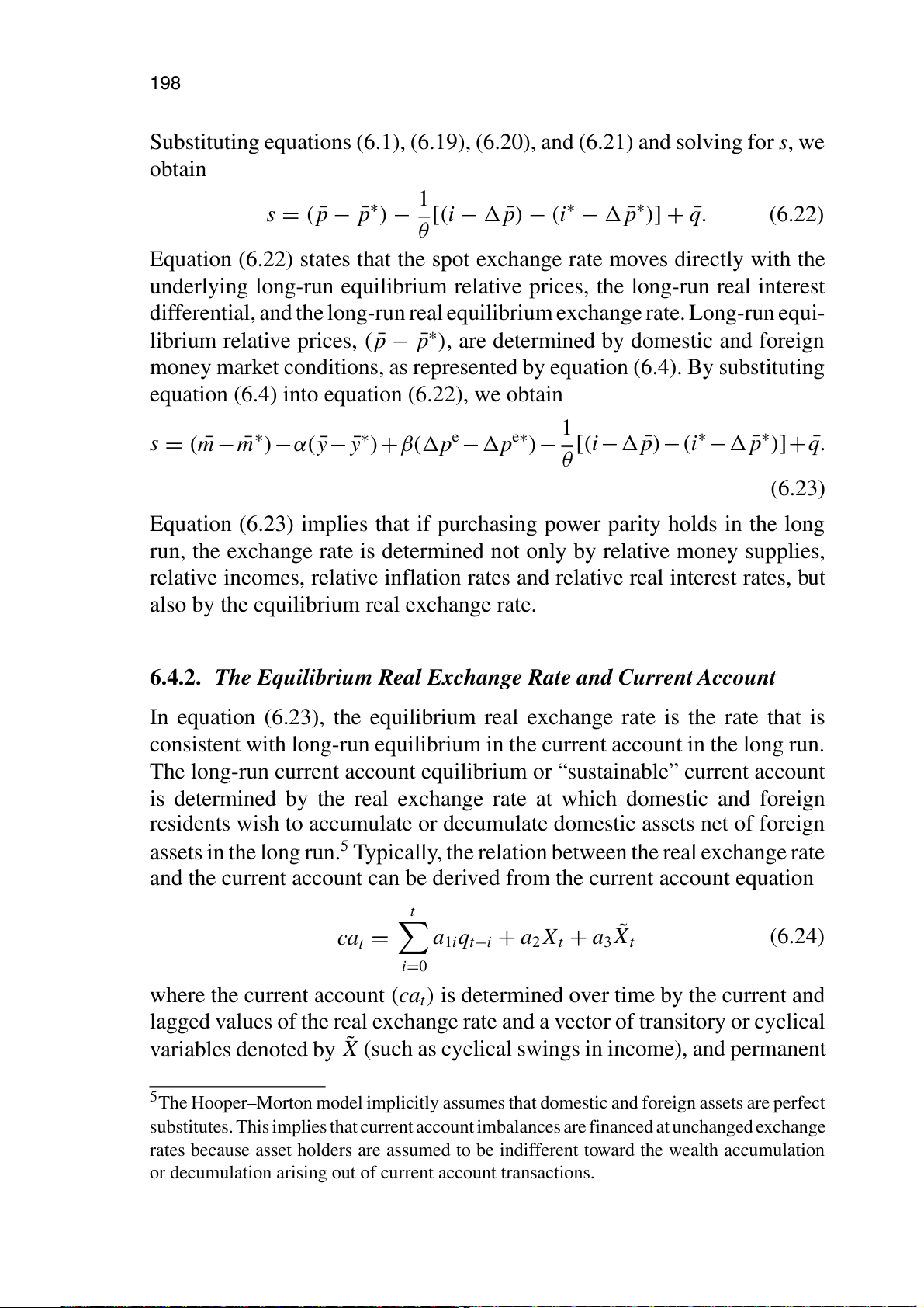
Substituting equations (6.1), (6.19), (6.20), and (6.21) and solving for s, we obtain 1 s = ( ¯ p − ¯ p∗) − [(i − ¯ p) − (i∗ − ¯ p∗)] + ¯ q. (6.22) θ
Equation (6.22) states that the spot exchange rate moves directly with the
underlying long-run equilibrium relative prices, the long-run real interest
differential, and the long-run real equilibrium exchange rate. Long-run equi- librium relative prices, ( ¯ p − ¯
p∗), are determined by domestic and foreign
money market conditions, as represented by equation (6.4). By substituting fic.com
equation (6.4) into equation (6.22), we obtain 1 s = ( ¯ m− ¯ m∗)−α( ¯ y − ¯
y∗)+β(pe −pe∗)− [(i− ¯ p)−(i∗ − ¯ p∗)]+ ¯ q. θ (6.23)
Equation (6.23) implies that if purchasing power parity holds in the long
run, the exchange rate is determined not only by relative money supplies,
relative incomes, relative inflation rates and relative real interest rates, but
also by the equilibrium real exchange rate.
6.4.2. The Equilibrium Real Exchange Rate and Current Account
In equation (6.23), the equilibrium real exchange rate is the rate that is
consistent with long-run equilibrium in the current account in the long run.
The long-run current account equilibrium or “sustainable” current account
is determined by the real exchange rate at which domestic and foreign
residents wish to accumulate or decumulate domestic assets net of foreign
assets in the long run.5 Typically, the relation between the real exchange rate
and the current account can be derived from the current account equation
by UNIVERSITY OF MELBOURNE on 01/13/17. For personal use only. t ca ˜ t = a1iqt−i + a2Xt + a3Xt (6.24)
The Theory and Empirics of Exchange Rates Downloaded from www.worldscienti i=0
where the current account (cat) is determined over time by the current and
lagged values of the real exchange rate and a vector of transitory or cyclical variables denoted by ˜
X (such as cyclical swings in income), and permanent
5The Hooper–Morton model implicitly assumes that domestic and foreign assets are perfect
substitutes. This implies that current account imbalances are financed at unchanged exchange
rates because asset holders are assumed to be indifferent toward the wealth accumulation
or decumulation arising out of current account transactions.
Other Sticky-Price Monetary Models of Exchange Rates 199
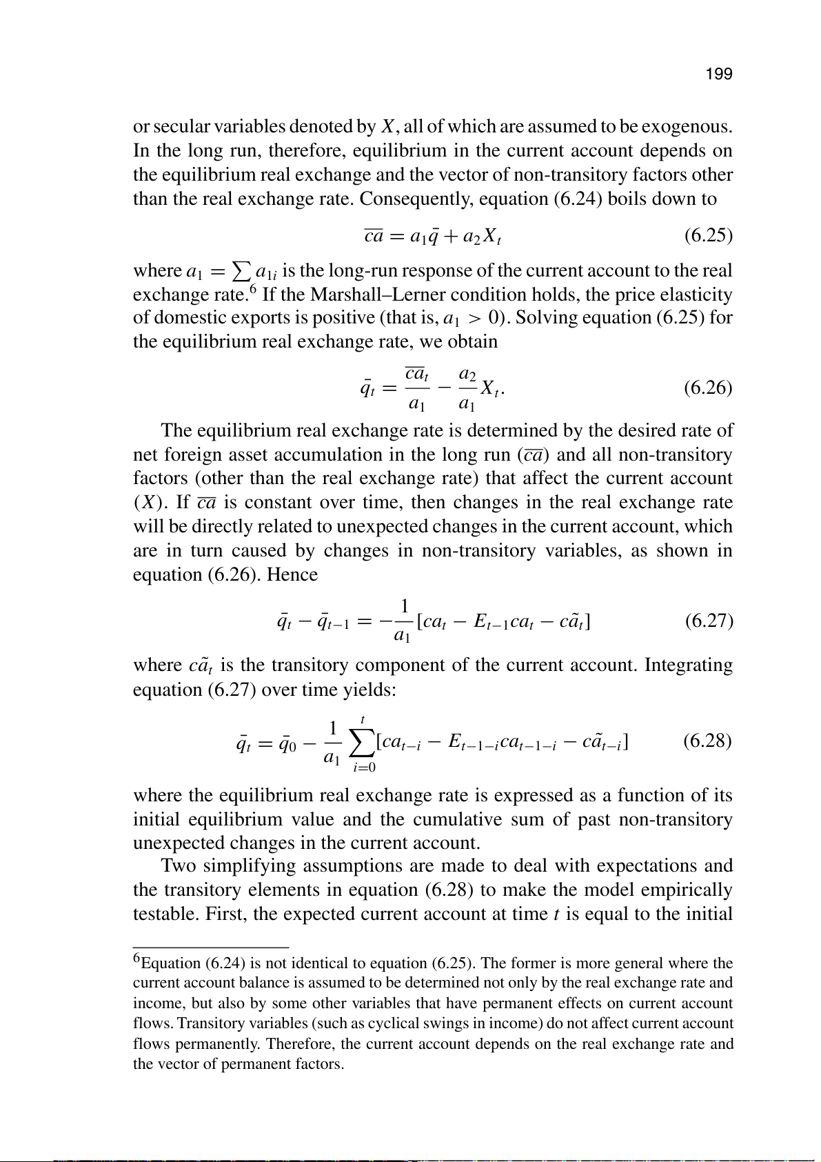
or secular variables denoted by X, all of which are assumed to be exogenous.
In the long run, therefore, equilibrium in the current account depends on
the equilibrium real exchange and the vector of non-transitory factors other
than the real exchange rate. Consequently, equation (6.24) boils down to ca = a1 ¯ q + a2Xt (6.25)
where a1 = a1i is the long-run response of the current account to the real
exchange rate.6 If the Marshall–Lerner condition holds, the price elasticity
of domestic exports is positive (that is, a1 > 0). Solving equation (6.25) for
the equilibrium real exchange rate, we obtain fic.com ca a ¯ t 2 qt = − Xt. (6.26) a1 a1
The equilibrium real exchange rate is determined by the desired rate of
net foreign asset accumulation in the long run (ca) and all non-transitory
factors (other than the real exchange rate) that affect the current account
(X). If ca is constant over time, then changes in the real exchange rate
will be directly related to unexpected changes in the current account, which
are in turn caused by changes in non-transitory variables, as shown in equation (6.26). Hence 1 ¯ qt − ¯ qt−1 = − [ca E c ˜ a a t − t−1cat − t ] (6.27) 1 where c ˜
at is the transitory component of the current account. Integrating
equation (6.27) over time yields: t 1 ¯ q [ t = ¯ q0 −
cat−i − Et−1−icat−1−i − c ˜ at−i] (6.28) a1 i=0
by UNIVERSITY OF MELBOURNE on 01/13/17. For personal use only.
where the equilibrium real exchange rate is expressed as a function of its
initial equilibrium value and the cumulative sum of past non-transitory
The Theory and Empirics of Exchange Rates Downloaded from www.worldscienti
unexpected changes in the current account.
Two simplifying assumptions are made to deal with expectations and
the transitory elements in equation (6.28) to make the model empirically
testable. First, the expected current account at time t is equal to the initial
6Equation (6.24) is not identical to equation (6.25). The former is more general where the
current account balance is assumed to be determined not only by the real exchange rate and
income, but also by some other variables that have permanent effects on current account
flows. Transitory variables (such as cyclical swings in income) do not affect current account
flows permanently. Therefore, the current account depends on the real exchange rate and
the vector of permanent factors. 200
The Theory and Empirics of Exchange Rates
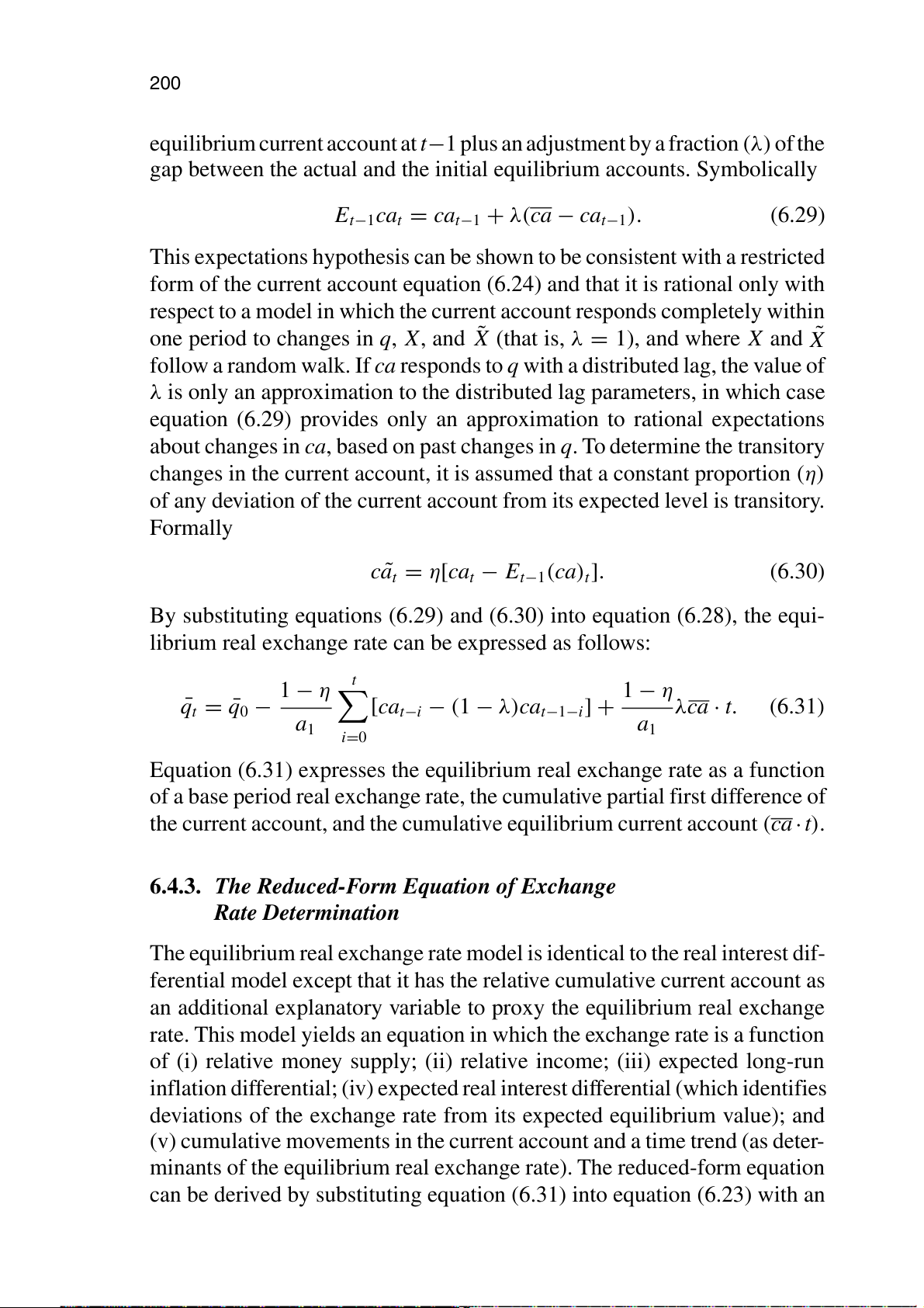
equilibrium current account at t−1 plus an adjustment by a fraction (λ) of the
gap between the actual and the initial equilibrium accounts. Symbolically
Et−1cat = cat−1 + λ(ca − cat−1). (6.29)
This expectations hypothesis can be shown to be consistent with a restricted
form of the current account equation (6.24) and that it is rational only with
respect to a model in which the current account responds completely within
one period to changes in q, X, and ˜
X (that is, λ = 1), and where X and ˜ X
follow a random walk. If ca responds to q with a distributed lag, the value of fic.com
λ is only an approximation to the distributed lag parameters, in which case
equation (6.29) provides only an approximation to rational expectations
about changes in ca, based on past changes in q. To determine the transitory
changes in the current account, it is assumed that a constant proportion (η)
of any deviation of the current account from its expected level is transitory. Formally c ˜ at = η[cat − Et−1(ca)t]. (6.30)
By substituting equations (6.29) and (6.30) into equation (6.28), the equi-
librium real exchange rate can be expressed as follows: t 1 − η 1 − η ¯ qt = ¯ q0 −
[cat−i − (1 − λ)cat−1−i] + λca · t. (6.31) a1 a1 i=0
Equation (6.31) expresses the equilibrium real exchange rate as a function
of a base period real exchange rate, the cumulative partial first difference of
the current account, and the cumulative equilibrium current account (ca · t).
6.4.3. The Reduced-Form Equation of Exchange
by UNIVERSITY OF MELBOURNE on 01/13/17. For personal use only.
Rate Determination
The Theory and Empirics of Exchange Rates Downloaded from www.worldscienti
The equilibrium real exchange rate model is identical to the real interest dif-
ferential model except that it has the relative cumulative current account as
an additional explanatory variable to proxy the equilibrium real exchange
rate. This model yields an equation in which the exchange rate is a function
of (i) relative money supply; (ii) relative income; (iii) expected long-run
inflation differential; (iv) expected real interest differential (which identifies
deviations of the exchange rate from its expected equilibrium value); and
(v) cumulative movements in the current account and a time trend (as deter-
minants of the equilibrium real exchange rate). The reduced-form equation
can be derived by substituting equation (6.31) into equation (6.23) with an
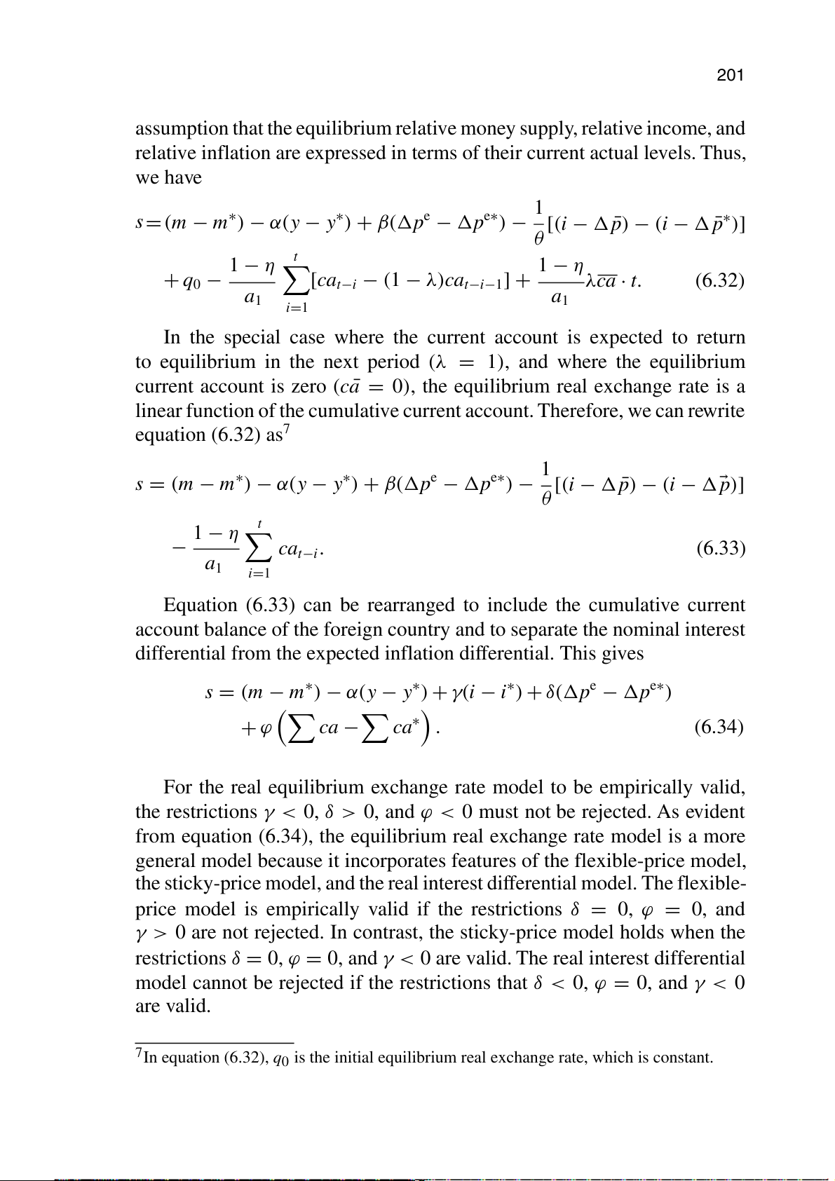
Other Sticky-Price Monetary Models of Exchange Rates 201
assumption that the equilibrium relative money supply, relative income, and
relative inflation are expressed in terms of their current actual levels. Thus, we have 1
s = (m − m∗) − α(y − y∗) + β(pe − pe∗) − [(i − ¯ p) − (i − ¯ p∗)] θ t 1 − η 1 − η + q0 −
[cat−i − (1 − λ)cat−i−1] + λca · t. (6.32) a1 a1 i=1
In the special case where the current account is expected to return fic.com
to equilibrium in the next period (λ = 1), and where the equilibrium current account is zero (c ¯
a = 0), the equilibrium real exchange rate is a
linear function of the cumulative current account. Therefore, we can rewrite equation (6.32) as7 1
s = (m − m∗) − α(y − y∗) + β(pe − pe∗) − [(i − ¯ p) − (i − p)] θ t 1 − η − cat−i. (6.33) a1 i=1
Equation (6.33) can be rearranged to include the cumulative current
account balance of the foreign country and to separate the nominal interest
differential from the expected inflation differential. This gives
s = (m − m∗) − α(y − y∗) + γ(i − i∗) + δ(pe − pe∗) + ϕ ca − ca∗ . (6.34)
For the real equilibrium exchange rate model to be empirically valid,
by UNIVERSITY OF MELBOURNE on 01/13/17. For personal use only.
the restrictions γ < 0, δ > 0, and ϕ < 0 must not be rejected. As evident
from equation (6.34), the equilibrium real exchange rate model is a more
The Theory and Empirics of Exchange Rates Downloaded from www.worldscienti
general model because it incorporates features of the flexible-price model,
the sticky-price model, and the real interest differential model. The flexible-
price model is empirically valid if the restrictions δ = 0, ϕ = 0, and
γ > 0 are not rejected. In contrast, the sticky-price model holds when the
restrictions δ = 0, ϕ = 0, and γ < 0 are valid. The real interest differential
model cannot be rejected if the restrictions that δ < 0, ϕ = 0, and γ < 0 are valid.
7In equation (6.32), q0 is the initial equilibrium real exchange rate, which is constant. 202
The Theory and Empirics of Exchange Rates
6.4.4. The Impact of the Risk Premium on the Exchange Rate
Portfolio preferences influence the exchange rate to the extent that they
play a role in the determination of the equilibrium real exchange rate (by
identifying the long-run current account). Now, we relax this assumption
and allow for imperfect substitutability of assets in the short run and the
existence of a risk premium, which gives E(s) = i − i∗ − ρ (6.35)
where ρ is the risk premium that asset holders demand on domestic assets fic.com
relative to foreign assets, given wealth, asset stocks, and the expected rel-
ative rates of return on those assets. Hooper and Morton (1982) employed
an abbreviated specification, expressing the risk premium as a linear
function of the cumulative current account, intervention flows, and an initial condition: T ρ = φ0 − φ1 (ca−j + I−j) (6.36) j=2
By allowing for the risk premium in equation (6.22), we obtain 1 ρ s = ¯ s − [(i − ¯ p) − (i∗ − ¯ p∗)] + ¯ q + . (6.37) θ θ
Substituting equations (6.37) and (6.31) into equation (6.23), we obtain s = ( ¯ m − ¯ m∗) − α( ¯ y − ¯ y∗) + β(pe − pe∗) 1 − [(i − ¯ p) − (i∗ − ¯ p∗)] + ¯ q0 θ t 1 − η
by UNIVERSITY OF MELBOURNE on 01/13/17. For personal use only. − [ca a
t−i − (1 − λ)cat−i−1] 1 i=1 T
The Theory and Empirics of Exchange Rates Downloaded from www.worldscienti 1 − η φ φ + 0 1 λca · t + − (ca−j + I−j). (6.38) a1 θ θ j=1
In equation (6.38), the current account affects the exchange rate via two
channels: expectations and short-run portfolio rebalancing. In the former
case, the announcement of a current account deficit (that is, unexpected and
nontransitory) affects the exchange rate (through changes in expectations
about the equilibrium exchange rate) in such a way as to restore long-
run equilibrium or a “sustainable” current account. In the latter case, if
Other Sticky-Price Monetary Models of Exchange Rates 203
the current account deficit is not financed by official intervention during
the length of time it takes to return to equilibrium, the necessary private
financing is attracted with an increase in the risk premium, which causes
the real exchange rate to overshoot its expected equilibrium level.
6.5. The Buiter–Miller Model with Core Inflation Rate
Buiter and Miller (1981) developed a variant of the Dornbusch (1976c)
sticky-price model that incorporates a core inflation rate, which is used to fic.com
analyze the dynamic effects of natural resource discoveries on output and
the exchange rate. Their analysis is designed to be suggestive of the U.K.’s
experience with the discovery of oil in the North Sea in the 1970s.
Buiter and Miller begin by specifying a money market equilibrium con-
dition, and a rational expectations augmented version of the UIP condition.
These two relations are written as mt − pt = φyt − λit (6.39) st+1 = (it − i∗). (6.40) t
In equation (6.40), the actual change in the exchange rate appears instead
of the expected change, reflecting the assumption of rational expectations.
The aggregate demand function explicitly incorporates the (negative) effect
of the real interest rate. Hence dt = α( ˙ pt − it) + β(st − pt). (6.41)
Inflation is assumed to be proportional to the level of excess demand over
the full employment level of output plus a core inflation rate:
by UNIVERSITY OF MELBOURNE on 01/13/17. For personal use only. ˙ pt = (dt − yt) + µt. (6.42)
The Theory and Empirics of Exchange Rates Downloaded from www.worldscienti
The core inflation rate (µ) is equal to the rate of growth in the money supply: µt = ˙ mt (6.43)
In the sticky-price monetary model, long-run equilibrium is achieved when
the current and long-run exchange rates are equal. In the Buiter–Miller
model, however, the presence of a core inflation rate implies a nonzero
difference between the current exchange rate and the long-run rate. This 204
The Theory and Empirics of Exchange Rates
result arises because, in equilibrium, the nominal interest rate is equal to
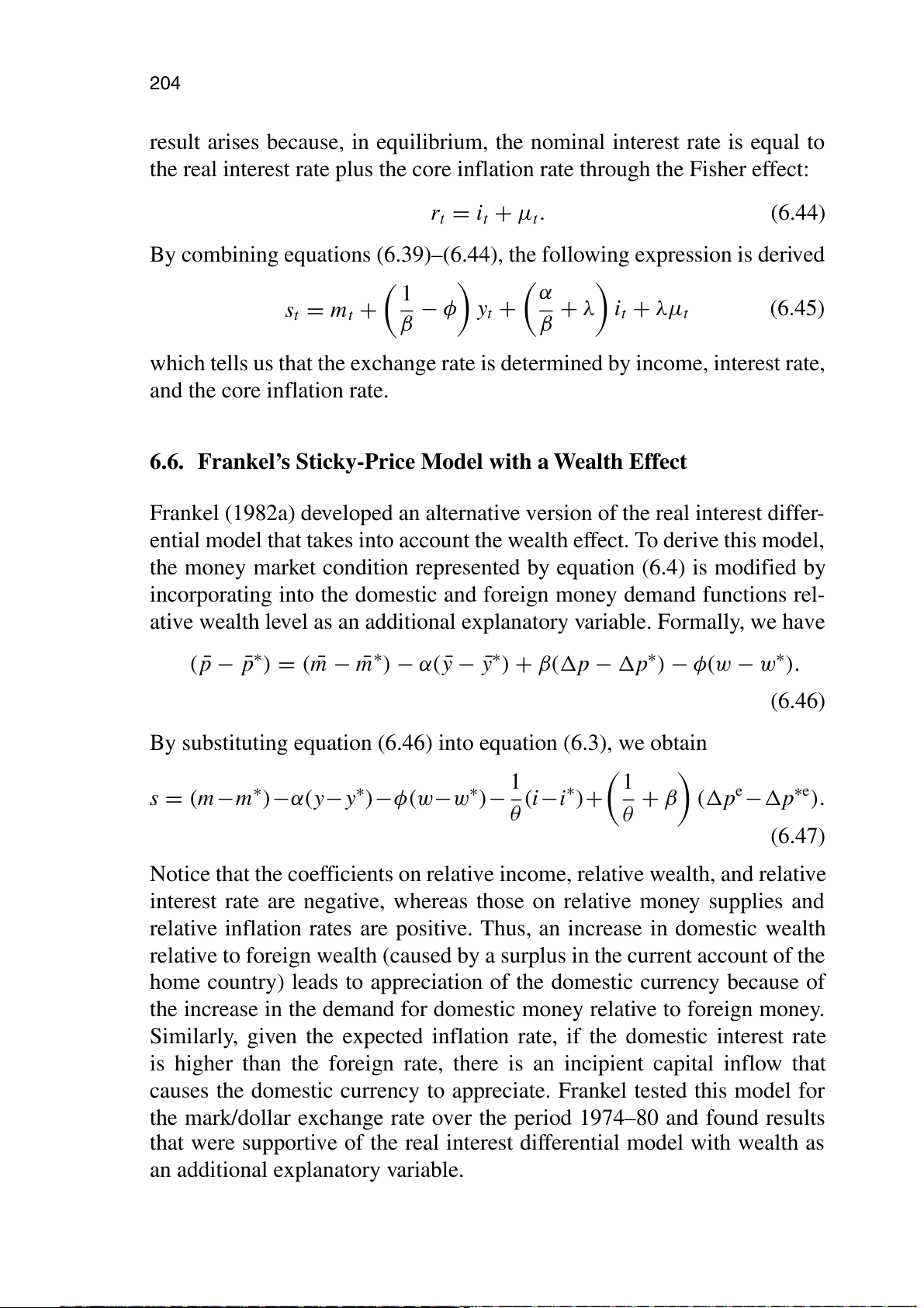
the real interest rate plus the core inflation rate through the Fisher effect: rt = it + µt. (6.44)
By combining equations (6.39)–(6.44), the following expression is derived 1 α s − + t = mt + φ yt + λ it + λµt (6.45) β β
which tells us that the exchange rate is determined by income, interest rate, fic.com and the core inflation rate.
6.6. Frankel’s Sticky-Price Model with a Wealth Effect
Frankel (1982a) developed an alternative version of the real interest differ-
ential model that takes into account the wealth effect. To derive this model,
the money market condition represented by equation (6.4) is modified by
incorporating into the domestic and foreign money demand functions rel-
ative wealth level as an additional explanatory variable. Formally, we have ( ¯ p − ¯ p∗) = ( ¯ m − ¯ m∗) − α( ¯ y − ¯
y∗) + β(p − p∗) − φ(w − w∗). (6.46)
By substituting equation (6.46) into equation (6.3), we obtain 1 1
s = (m−m∗)−α(y−y∗)−φ(w−w∗)− (i−i∗)+ + β (pe −p∗e). θ θ (6.47)
Notice that the coefficients on relative income, relative wealth, and relative
by UNIVERSITY OF MELBOURNE on 01/13/17. For personal use only.
interest rate are negative, whereas those on relative money supplies and
relative inflation rates are positive. Thus, an increase in domestic wealth
The Theory and Empirics of Exchange Rates Downloaded from www.worldscienti
relative to foreign wealth (caused by a surplus in the current account of the
home country) leads to appreciation of the domestic currency because of
the increase in the demand for domestic money relative to foreign money.
Similarly, given the expected inflation rate, if the domestic interest rate
is higher than the foreign rate, there is an incipient capital inflow that
causes the domestic currency to appreciate. Frankel tested this model for
the mark/dollar exchange rate over the period 1974–80 and found results
that were supportive of the real interest differential model with wealth as
an additional explanatory variable.
Other Sticky-Price Monetary Models of Exchange Rates 205 6.7. Recapitulation
The sticky-price monetary model of Dornbusch allows substantial short-
term overshooting of nominal and real exchange rates beyond the long-
run equilibrium values determined by purchasing power parity because the
“jump variables” in the system (exchange rates and interest rates) com-
pensate for sluggishness in other variables, notably goods prices. This model
is a representation of long-run equilibrium toward which the economy tends
to adjust, while in the short run it is possible for the exchange rate to over- shoot its long-run value. fic.com
During the late 1970s and early 1980s, a wide range of sticky-price
models were developed to account for some observations pertaining to the
behavior of flexible exchange rates. These models include the real interest
differential model of Frankel (1979b), the stock-flow model of Driskell
(1981), and the equilibrium real exchange rate sticky-price model of Hooper
and Morton (1982). While these models appeared to have made some useful
additions to the Dornbusch model, their empirical validity remained as
questionable as their predecessors.
by UNIVERSITY OF MELBOURNE on 01/13/17. For personal use only.
The Theory and Empirics of Exchange Rates Downloaded from www.worldscienti
Tài liệu liên quan:
-

Hoạt động Tài chính của Doanh nghiệp Đa Quốc Gia (DN) - Chương 6 | Tài chính quốc tế | Trường Học Viện nông nghiệp Việt Nam
19 10 -

Hệ Thống Tiền Tệ Quốc Tế: Khái Niệm và Các Chế Độ Tỷ Giá | Tài chính quốc tế | Trường Học Viện nông nghiệp Việt Nam
24 12 -

Bài giảng Chương 1: Các Quan Hệ Cân Bằng Quốc Tế và LOP | Tài chính quốc tế | Trường Học Viện nông nghiệp Việt Nam
21 11 -
Cách Tính Lạm Phát và CPI: So Sánh Việt Nam và Mỹ | Tài chính quốc tế | Trường Học Viện nông nghiệp Việt Nam
23 12 -

Detailed Report and Analysis on Submission Trends | Tài chính quốc tế | Trường Học Viện nông nghiệp Việt Nam
23 12