The cellular concept — System design fundamentals môn Thông tin di động | Trường Đại học Bách Khoa Hà Nội
The cellular concept was a major breakthrough in solving the problem of spectral congestion and user capacity. It offered very high capacity in a limited spectrum allocation without any major technological changes. Tài liệu được sưu tầm gồm 57 trang, giúp các bạn nắm vững kiến thức, rèn luyện kỹ năng và đạt được kết quả tốt trong học tập. Mời các bạn đón xem!
Môn: Thông tin di động 14 tài liệu
Trường: Đại học Bách Khoa Hà Nội 5.6 K tài liệu
Tác giả:


Preview text:
lOMoAR cPSD| 59671932 0 C HAPTER 3 The Cellular Concept—
System Design Fundamentals T
he design objective of early mobile radio systems was to achieve a large coverage area
by using a single, high powered transmitter with an antenna mounted on a tall tower. While this
approach achieved very good coverage, it also meant that it was impossible to reuse those same
frequencies throughout the system, since any attempts to achieve frequency reuse would result in
interference. For example, the Bell mobile system in New York City in the 1970s could only
support a maximum of twelve simultaneous calls over a thousand square miles [Cal88]. Faced
with the fact that government regulatory agencies could not make spectrum allocations in
proportion to the increasing demand for mobile services, it became imperative to restructure the
radio telephone system to achieve high capacity with limited radio spectrum while at the same
time covering very large areas. 3.1 Introduction
The cellular concept was a major breakthrough in solving the problem of spectral congestion and
user capacity. It offered very high capacity in a limited spectrum allocation without any major
technological changes. The cellular concept is a system-level idea which calls for replacing a
single, high power transmitter (large cell) with many low power transmitters (small cells), each
providing coverage to only a small portion of the service area. Each base station is allocated a
portion of the total number of channels available to the entire system, and nearby base stations
are assigned different groups of channels so that all the available channels are assigned to a lOMoAR cPSD| 59671932 0
relatively small number of neighboring base stations. Neighboring base stations are assigned
different groups of channels so that the interference between base stations (and the mobile users
under their control) is minimized. By systematically spacing base stations and their channel 57 58
groups throughout a market, the available channels are distributed throughout the geographic
region and may be reused as many times as necessary so long as the interference between
cochannel stations is kept below acceptable levels.
As the demand for service increases (i.e., as more channels are needed within a particular
market), the number of base stations may be increased (along with a corresponding decrease in
transmitter power to avoid added interference), thereby providing additional radio capacity with
no additional increase in radio spectrum. This fundamental principle is the foundation for all
modern wireless communication systems, since it enables a fixed number of channels to serve an
arbitrarily large number of subscribers by reusing the channels throughout the coverage region.
Furthermore, the cellular concept allows every piece of subscriber equipment within a country or
continent to be manufactured with the same set of channels so that any mobile may be used anywhere within the region. 3.2 Frequency Reuse
Cellular radio systems rely on an intelligent allocation and reuse of channels throughout a
coverage region [Oet83]. Each cellular base station is allocated a group of radio channels to be
used within a small geographic area called a cell. Base stations in adjacent cells are assigned
channel groups which contain completely different channels than neighboring cells. The base
station antennas are designed to achieve the desired coverage within the particular cell. By
limiting the coverage area to within the boundaries of a cell, the same group of channels may be
used to cover different cells that are separated from one another by distances large enough to keep
interference levels within tolerable limits. The design process of selecting and allocating channel
groups for all of the cellular base stations within a system is called frequency reuse or frequency planning [Mac79].
Figure 3.1 illustrates the concept of cellular frequency reuse, where cells labeled with the
same letter use the same group of channels. The frequency reuse plan is overlaid upon a map to
indicate where different frequency channels are used. The hexagonal cell shape shown in Figure
3.1 is conceptual and is a simplistic model of the radio coverage for each base station, but it has
been universally adopted since the hexagon permits easy and manageable analysis of a cellular
system. The actual radio coverage of a cell is known as the footprint and is determined from field
measurements or propagation prediction models. Although the real footprint is amorphous in
nature, a regular cell shape is needed for systematic system design and adaptation for future
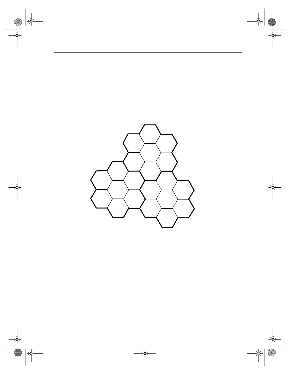
growth. While it might seem natural to choose a circle to represent the coverage area of a base lOMoAR cPSD| 59671932 0
station, adjacent circles cannot be overlaid upon a map without leaving gaps or creating
overlapping regions. Thus, when considering geometric shapes which cover an entire region
without overlap and with equal area, there are three sensible choices—a square, an equilateral
triangle, and a hexagon. A cell must be designed to serve the weakest mobiles within the footprint,
and these are typically located at the edge of the cell. For a given distance between the center of
a polygon and its farthest perimeter points, the hexagon has the largest area of the three. Thus, by
using the hexagon geometry, the fewest number of cells can cover a geographic region, and the
hexagon closely approximates a circular radiation pattern which would occur for an omnidirectional base Frequency Reuse 59 B G C A F D B E G C B A G C F D A E F D E
Figure 3.1 Illustration of the cellular frequency reuse concept. Cells with the same letter use the
same set of frequencies. A cel cluster is outlined in bold and replicated over the coverage area.
In this example, the cluster size, N, is equal to seven, and the frequency reuse factor is 1/7 since
each cell contains one-seventh of the total number of available channels.
station antenna and free space propagation. Of course, the actual cellular footprint is determined
by the contour in which a given transmitter serves the mobiles successfully.
When using hexagons to model coverage areas, base station transmitters are depicted as
either being in the center of the cell (center-excited cells) or on three of the six cell vertices (edge-
excited cells). Normally, omnidirectional antennas are used in center-excited cells and sectored
directional antennas are used in corner-excited cells. Practical considerations usually do not allow
base stations to be placed exactly as they appear in the hexagonal layout. Most system designs
permit a base station to be positioned up to one-fourth the cell radius away from the ideal location. lOMoAR cPSD| 59671932 0
To understand the frequency reuse concept, consider a cellular system which has a total of
S duplex channels available for use. If each cell is allocated a group of k channels (k < S), and if
the S channels are divided among N cells into unique and disjoint channel groups which each
have the same number of channels, the total number of available radio channels can be expressed as S = kN (3.1)
The N cells which collectively use the complete set of available frequencies is called a
cluster. If a cluster is replicated M times within the system, the total number of duplex channels,
C, can be used as a measure of capacity and is given by
C = MkN = MS (3.2) 60
As seen from Equation (3.2), the capacity of a cellular system is directly proportional to the
number of times a cluster is replicated in a fixed service area. The factor N is called the cluster
size and is typically equal to 4, 7, or 12. If the cluster size N is reduced while the cell size is kept
constant, more clusters are required to cover a given area, and hence more capacity (a larger value
of C) is achieved. A large cluster size indicates that the ratio between the cell radius and the
distance between co-channel cells is small. Conversely, a small cluster size indicates that co-
channel cells are located much closer together. The value for N is a function of how much
interference a mobile or base station can tolerate while maintaining a sufficient quality of
communications. From a design viewpoint, the smallest possible value of N is desirable in order
to maximize capacity over a given coverage area (i.e., to maximize C in Equation (3.2)). The
frequency reuse factor of a cellular system is given by 1/N, since each cell within a cluster is only
assigned 1/N of the total available channels in the system.
Due to the fact that the hexagonal geometry of Figure 3.1 has exactly six equidistant
neighbors and that the lines joining the centers of any cell and each of its neighbors are separated
by multiples of 60 degrees, there are only certain cluster sizes and cell layouts which are possible
[Mac79]. In order to tessellate—to connect without gaps between adjacent cells—the geometry
of hexagons is such that the number of cells per cluster, N, can only have values which satisfy Equation (3.3). 2 2
N = i + ij + j (3.3)
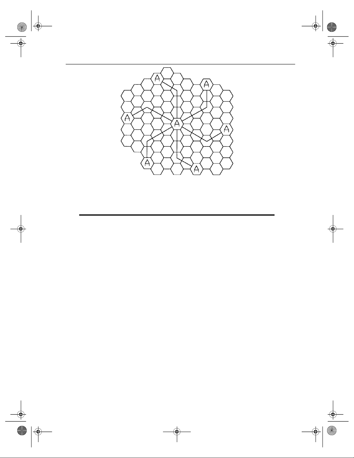
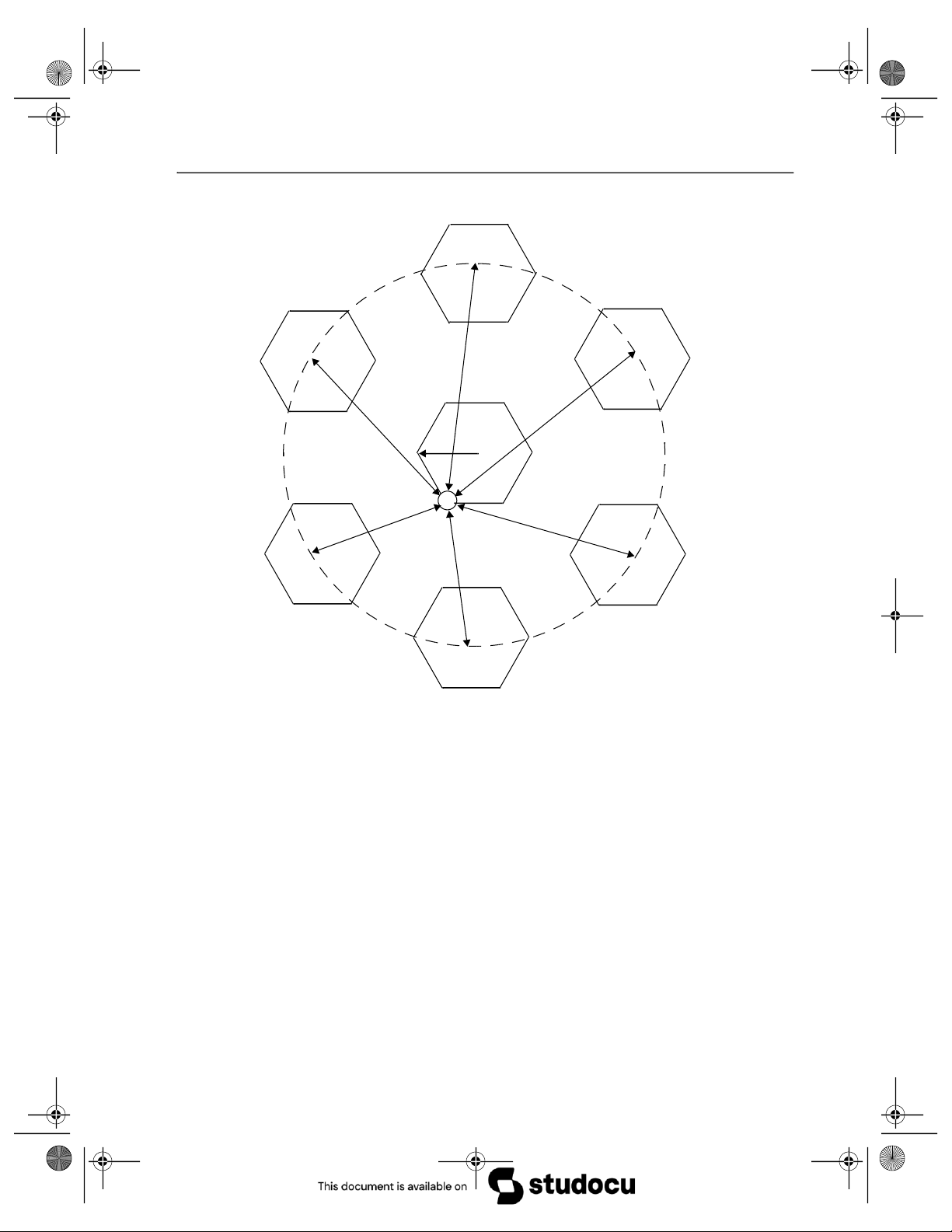
where i and j are non-negative integers. To find the nearest co-channel neighbors of a particular
cell, one must do the following: (1) move i cells along any chain of hexagons and then (2) turn
60 degrees counter-clockwise and move j cells. This is illustrated in Figure 3.2 for i = 3 and j = 2 (example, N = 19). lOMoAR cPSD| 59671932 0 Figure 3.2
Method of locating co-channel cells in a cel ular system. In this example, N = 19
(i.e., i= 3, j = 2). (Adapted from [Oet83] © IEEE.) Frequency Reuse 61 Example 3.1
If a total of 33 MHz of bandwidth is allocated to a particular FDD cellular telephone
system which uses two 25 kHz simplex channels to provide full duplex voice and
control channels, compute the number of channels available per cell if a system uses
(a) four-cell reuse, (b) seven-cell reuse, and (c) 12-cell reuse. If 1 MHz of the al ocated
spectrum is dedicated to control channels, determine an equitable distribution of
control channels and voice channels in each cell for each of the three systems. Solution Given: Total bandwidth = 33 MHz
Channel bandwidth = 25 kHz × 2 simplex channels = 50 kHz/duplex channel
Total available channels = 33,000/50 = 660 channels
(a) For N = 4, total number of channels available per cell = 660/4 ≈ 165 channels.
(b) For N = 7, total number of channels available per cel = 660/7 ≈ 95 channels.
(c) For N = 12, total number of channels available per cell = 660/12 ≈ 55 channels.
A 1 MHz spectrum for control channels implies that there are 1000/50 = 20 control
channels out of the 660 channels available. To evenly distribute the control and voice
channels, simply al ocate the same number of voice channels in each cel wherever
possible. Here, the 660 channels must be evenly distributed to each cell within the
cluster. In practice, only the 640 voice channels would be allocated, since the control
channels are al ocated separately as 1 per cell. lOMoAR cPSD| 59671932 0
(a) For N = 4, we can have five control channels and 160 voice channels per cel . In
practice, however, each cell only needs a single control channel (the control channels
have a greater reuse distance than the voice channels). Thus, one control channel
and 160 voice channels would be assigned to each cell.
(b) For N = 7, four cells with three control channels and 92 voice channels, two cells
with three control channels and 90 voice channels, and one cell with two control
channels and 92 voice channels could be allocated. In practice, however, each cell
would have one control channel, four cells would have 91 voice channels, and three
cells would have 92 voice channels.
(c) For N = 12, we can have eight cells with two control channels and 53 voice
channels, and four cel s with one control channel and 54 voice channels each. In an
actual system, each cel would have one control channel, eight cells would have 53
voice channels, and four cel s would have 54 voice channels. 62
3.3 Channel Assignment Strategies
For efficient utilization of the radio spectrum, a frequency reuse scheme that is consistent with
the objectives of increasing capacity and minimizing interference is required. A variety of channel
assignment strategies have been developed to achieve these objectives. Channel assignment
strategies can be classified as either fixed or dynamic. The choice of channel assignment strategy
impacts the performance of the system, particularly as to how calls are managed when a mobile
user is handed off from one cell to another [Tek91], [LiC93], [Sun94], [Rap93b].
In a fixed channel assignment strategy, each cell is allocated a predetermined set of voice
channels. Any call attempt within the cell can only be served by the unused channels in that
particular cell. If all the channels in that cell are occupied, the call is blocked and the subscriber
does not receive service. Several variations of the fixed assignment strategy exist. In one
approach, called the borrowing strategy, a cell is allowed to borrow channels from a neighboring
cell if all of its own channels are already occupied. The mobile switching center (MSC) supervises
such borrowing procedures and ensures that the borrowing of a channel does not disrupt or
interfere with any of the calls in progress in the donor cell.
In a dynamic channel assignment strategy, voice channels are not allocated to different cells
permanently. Instead, each time a call request is made, the serving base station requests a channel
from the MSC. The switch then allocates a channel to the requested cell following an algorithm
that takes into account the likelihood of future blocking within the cell, the frequency of use of
the candidate channel, the reuse distance of the channel, and other cost functions.
Accordingly, the MSC only allocates a given frequency if that frequency is not presently
in use in the cell or any other cell which falls within the minimum restricted distance of frequency
reuse to avoid co-channel interference. Dynamic channel assignment reduce the likelihood of
blocking, which increases the trunking capacity of the system, since all the available channels in
a market are accessible to all of the cells. Dynamic channel assignment strategies require the lOMoAR cPSD| 59671932 0
MSC to collect real-time data on channel occupancy, traffic distribution, and radio signal strength
indications (RSSI) of all channels on a continuous basis. This increases the storage and
computational load on the system but provides the advantage of increased channel utilization and
decreased probability of a blocked call. 3.4 Handoff Strategies
When a mobile moves into a different cell while a conversation is in progress, the MSC
automatically transfers the call to a new channel belonging to the new base station. This handoff
operation not only involves identifying a new base station, but also requires that the voice and
control signals be allocated to channels associated with the new base station.
Processing handoffs is an important task in any cellular radio system. Many handoff
strategies prioritize handoff requests over call initiation requests when allocating unused channels
in a cell site. Handoffs must be performed successfully and as infrequently as possible, and be
imperceptible to the users. In order to meet these requirements, system designers must specify an
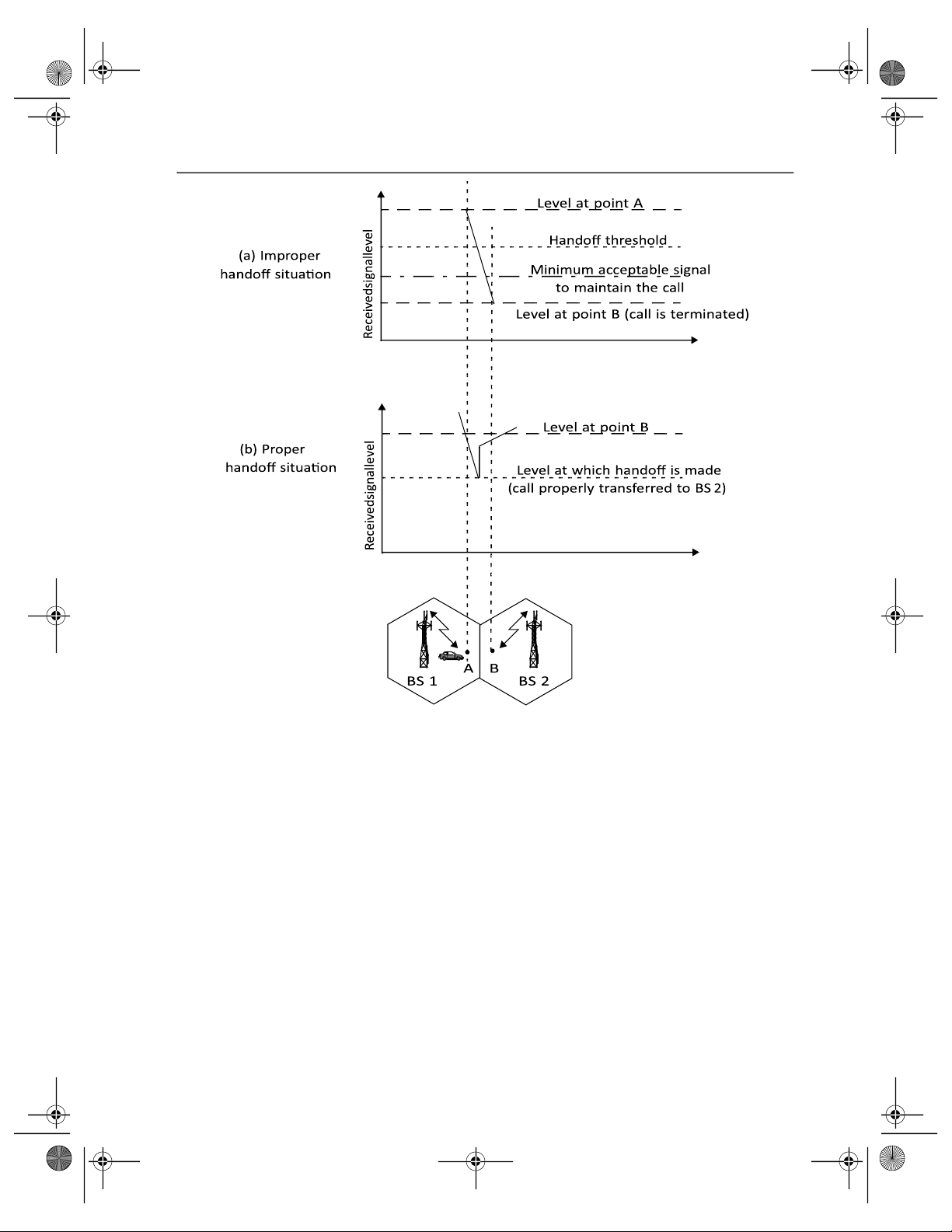
optimum signal level at which to initiate a handoff. Once a particular signal level is specified as the minimum usable Handoff Strategies 63
signal for acceptable voice quality at the base station receiver (normally taken as between –90
dBm and –100 dBm), a slightly stronger signal level is used as a threshold at which a handoff is made.
This margin, given by ∆ = Pr handoff – Pr minimum usable, cannot be too large or too small. If ∆ is too
large, unnecessary handoffs which burden the MSC may occur, and if ∆ is too small, there may
be insufficient time to complete a handoff before a call is lost due to weak signal conditions.
Therefore, ∆ is chosen carefully to meet these conflicting requirements. Figure 3.3 illustrates a
handoff situation. Figure 3.3(a) demonstrates the case where a handoff is not made and the signal
drops below the minimum acceptable level to keep the channel active. This dropped call event
can happen when there is an excessive delay by the MSC in assigning a handoff or when the
threshold ∆ is set too small for the handoff time in the system. Excessive delays may occur during
high traffic conditions due to computational loading at the MSC or due to the fact that no channels
are available on any of the nearby base stations (thus forcing the MSC to wait until a channel in a nearby cell becomes free). lOMoAR cPSD| 59671932 0 Time Time
Figure 3.3 Illustration of a handoff scenario at cel boundary. 64
In deciding when to handoff, it is important to ensure that the drop in the measured signal
level is not due to momentary fading and that the mobile is actually moving away from the serving
base station. In order to ensure this, the base station monitors the signal level for a certain period
of time before a handoff is initiated. This running average measurement of signal strength should
be optimized so that unnecessary handoffs are avoided, while ensuring that necessary handoffs
are completed before a call is terminated due to poor signal level. The length of time needed to
decide if a handoff is necessary depends on the speed at which the vehicle is moving. If the slope
of the short-term average received signal level in a given time interval is steep, the handoff should
be made quickly. Information about the vehicle speed, which can be useful in handoff decisions,
can also be computed from the statistics of the received short-term fading signal at the base station.
The time over which a call may be maintained within a cell, without handoff, is called the
dwell time [Rap93b]. The dwell time of a particular user is governed by a number of factors, lOMoAR cPSD| 59671932 0
including propagation, interference, distance between the subscriber and the base station, and
other time varying effects. Chapter 5 shows that even when a mobile user is stationary, ambient
motion in the vicinity of the base station and the mobile can produce fading; thus, even a
stationary subscriber may have a random and finite dwell time. Analysis in [Rap93b] indicates
that the statistics of dwell time vary greatly, depending on the speed of the user and the type of
radio coverage. For example, in mature cells which provide coverage for vehicular highway users,
most users tend to have a relatively constant speed and travel along fixed and well-defined paths
with good radio coverage. In such instances, the dwell time for an arbitrary user is a random
variable with a distribution that is highly concentrated about the mean dwell time. On the other
hand, for users in dense, cluttered microcell environments, there is typically a large variation of
dwell time about the mean, and the dwell times are typically shorter than the cell geometry would
otherwise suggest. It is apparent that the statistics of dwell time are important in the practical
design of handoff algorithms [LiC93], [Sun94], [Rap93b].
In first generation analog cellular systems, signal strength measurements are made by the
base stations and supervised by the MSC. Each base station constantly monitors the signal
strengths of all of its reverse voice channels to determine the relative location of each mobile user
with respect to the base station tower. In addition to measuring the RSSI of calls in progress
within the cell, a spare receiver in each base station, called the locator receiver, is used to scan
and determine signal strengths of mobile users which are in neighboring cells. The locator
receiver is controlled by the MSC and is used to monitor the signal strength of users in
neighboring cells which appear to be in need of handoff and reports all RSSI values to the MSC.
Based on the locator receiver signal strength information from each base station, the MSC decides
if a handoff is necessary or not.
In today’s second generation systems, handoff decisions are mobile assisted. In mobile
assisted handoff (MAHO), every mobile station measures the received power from surrounding
base stations and continually reports the results of these measurements to the serving base station.
A handoff is initiated when the power received from the base station of a neighboring cell begins
to exceed the power received from the current base station by a certain level or for a certain period of Handoff Strategies 65
time. The MAHO method enables the call to be handed over between base stations at a much
faster rate than in first generation analog systems since the handoff measurements are made by
each mobile, and the MSC no longer constantly monitors signal strengths. MAHO is particularly
suited for microcellular environments where handoffs are more frequent.
During the course of a call, if a mobile moves from one cellular system to a different cellular
system controlled by a different MSC, an intersystem handoff becomes necessary. An MSC
engages in an intersystem handoff when a mobile signal becomes weak in a given cell and the
MSC cannot find another cell within its system to which it can transfer the call in progress. There
are many issues that must be addressed when implementing an intersystem handoff. For instance, lOMoAR cPSD| 59671932 0
a local call may become a long-distance call as the mobile moves out of its home system and
becomes a roamer in a neighboring system. Also, compatibility between the two MSCs must be
determined before implementing an intersystem handoff. Chapter 10 demonstrates how
intersystem handoffs are implemented in practice.
Different systems have different policies and methods for managing handoff requests. Some
systems handle handoff requests in the same way they handle originating calls. In such systems,
the probability that a handoff request will not be served by a new base station is equal to the
blocking probability of incoming calls. However, from the user’s point of view, having a call
abruptly terminated while in the middle of a conversation is more annoying than being blocked
occasionally on a new call attempt. To improve the quality of service as perceived by the users,
various methods have been devised to prioritize handoff requests over call initiation requests
when allocating voice channels.
3.4.1 Prioritizing Handoffs
One method for giving priority to handoffs is called the guard channel concept, whereby a
fraction of the total available channels in a cell is reserved exclusively for handoff requests from
ongoing calls which may be handed off into the cell. This method has the disadvantage of
reducing the total carried traffic, as fewer channels are allocated to originating calls. Guard
channels, however, offer efficient spectrum utilization when dynamic channel assignment
strategies, which minimize the number of required guard channels by efficient demand-based allocation, are used.
Queuing of handoff requests is another method to decrease the probability of forced
termination of a call due to lack of available channels. There is a tradeoff between the decrease
in probability of forced termination and total carried traffic. Queuing of handoffs is possible due
to the fact that there is a finite time interval between the time the received signal level drops
below the handoff threshold and the time the call is terminated due to insufficient signal level.
The delay time and size of the queue is determined from the traffic pattern of the particular service
area. It should be noted that queuing does not guarantee a zero probability of forced termination,
since large delays will cause the received signal level to drop below the minimum required level
to maintain communication and hence lead to forced termination. 66
3.4.2 Practical Handoff Considerations
In practical cellular systems, several problems arise when attempting to design for a wide range
of mobile velocities. High speed vehicles pass through the coverage region of a cell within a
matter of seconds, whereas pedestrian users may never need a handoff during a call. Particularly
with the addition of microcells to provide capacity, the MSC can quickly become burdened if
high speed users are constantly being passed between very small cells. Several schemes have
been devised to handle the simultaneous traffic of high speed and low speed users while lOMoAR cPSD| 59671932 0
minimizing the handoff intervention from the MSC. Another practical limitation is the ability to obtain new cell sites.
Although the cellular concept clearly provides additional capacity through the addition of
cell sites, in practice it is difficult for cellular service providers to obtain new physical cell site
locations in urban areas. Zoning laws, ordinances, and other nontechnical barriers often make it
more attractive for a cellular provider to install additional channels and base stations at the same
physical location of an existing cell, rather than find new site locations. By using different antenna
heights (often on the same building or tower) and different power levels, it is possible to provide
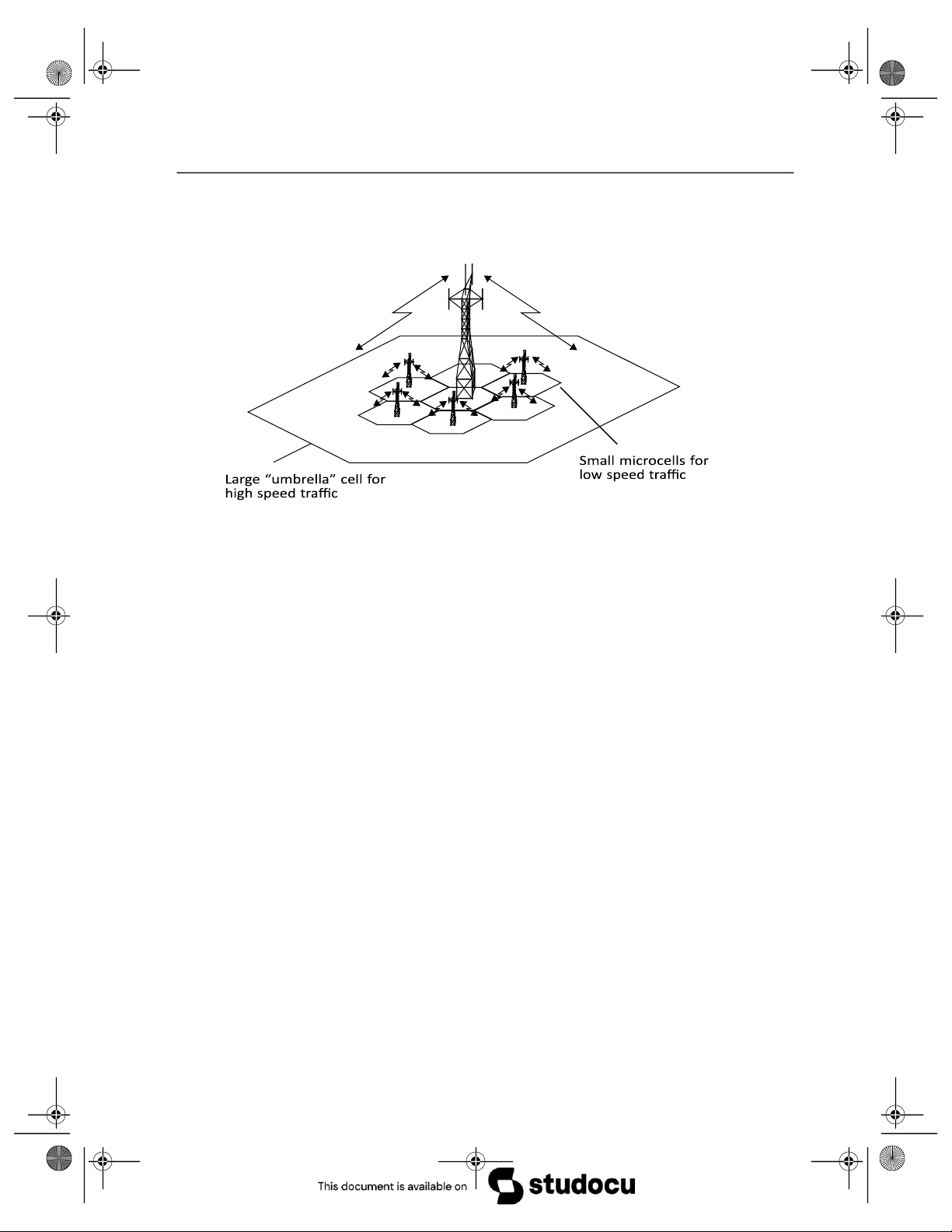
“large” and “small” cells which are co-located at a single location. This technique is called the
umbrella cell approach and is used to provide large area coverage to high speed users while
providing small area coverage to users traveling at low speeds. Figure 3.4 illustrates an umbrella
cell which is colocated with some smaller microcells. The umbrella cell approach ensures that
the number of handoffs is minimized for high speed users and provides additional microcell
channels for pedestrian users. The speed of each user may be estimated by the base station or
MSC by evaluating how rapidly the short-term average signal strength on the RVC changes over
time, or more sophisticated algorithms may be used to evaluate and partition users [LiC93]. If a
high speed user in the large umbrella cell is approaching the base station, and its velocity is rapidly
decreasing, the base station may decide to hand the user into the co-located microcell, without MSC intervention.
Another practical handoff problem in microcell systems is known as cell dragging. Cell
dragging results from pedestrian users that provide a very strong signal to the base station. Such
a situation occurs in an urban environment when there is a line-of-sight (LOS) radio path between
the subscriber and the base station. As the user travels away from the base station at a very slow
speed, the average signal strength does not decay rapidly. Even when the user has traveled well
beyond the designed range of the cell, the received signal at the base station may be above the
handoff threshold, thus a handoff may not be made. This creates a potential interference and
traffic management problem, since the user has meanwhile traveled deep within a neighboring
cell. To solve the cell dragging problem, handoff thresholds and radio coverage parameters must be adjusted carefully.
In first generation analog cellular systems, the typical time to make a handoff, once the
signal level is deemed to be below the handoff threshold, is about 10 seconds. This requires that
the value for ∆ be on the order of 6 dB to 12 dB. In digital cellular systems such as GSM, the
mobile assists with the handoff procedure by determining the best handoff candidates, and the
handoff, once the decision is made, typically requires only 1 or 2 seconds. Consequently, ∆ is lOMoAR cPSD| 59671932
03_57_104_final.fm Page 68 Tuesday, December 4, 2001 2:17 PM
Interference and System Capacity 67
Figure 3.4 The umbrella cell approach.
usually between 0 dB and 6 dB in modern cellular systems. The faster handoff process supports
a much greater range of options for handling high speed and low speed users and provides the
MSC with substantial time to “rescue” a call that is in need of handoff.
Another feature of newer cellular systems is the ability to make handoff decisions based on
a wide range of metrics other than signal strength. The co-channel and adjacent channel
interference levels may be measured at the base station or the mobile, and this information may
be used with conventional signal strength data to provide a multi-dimensional algorithm for
determining when a handoff is needed.
The IS-95 code division multiple access (CDMA) spread spectrum cellular system
described in Chapter 11 and in [Lib99], [Kim00], and [Gar99], provides a unique handoff
capability that cannot be provided with other wireless systems. Unlike channelized wireless
systems that assign different radio channels during a handoff (called a hard handoff), spread
spectrum mobiles share the same channel in every cell. Thus, the term handoff does not mean a
physical change in the assigned channel, but rather that a different base station handles the radio
communication task. By simultaneously evaluating the received signals from a single subscriber
at several neighboring base stations, the MSC may actually decide which version of the user’s
signal is best at any moment in time. This technique exploits macroscopic space diversity
provided by the different physical locations of the base stations and allows the MSC to make a
“soft” decision as to which version of the user’s signal to pass along to the PSTN at any instance
[Pad94]. The ability to select between the instantaneous received signals from a variety of base
stations is called soft handoff.
Downloaded by Uc Lan (uehbsaxac464@gmail.com) lOMoAR cPSD| 59671932
03_57_104_final.fm Page 69 Tuesday, December 4, 2001 2:17 PM
Interference and System Capacity
3.5 Interference and System Capacity
Interference is the major limiting factor in the performance of cellular radio systems. Sources of
interference include another mobile in the same cell, a call in progress in a neighboring cell, other
base stations operating in the same frequency band, or any noncellular system which inadvertently 68
leaks energy into the cellular frequency band. Interference on voice channels causes cross talk,
where the subscriber hears interference in the background due to an undesired transmission. On
control channels, interference leads to missed and blocked calls due to errors in the digital
signaling. Interference is more severe in urban areas, due to the greater RF noise floor and the
large number of base stations and mobiles. Interference has been recognized as a major bottleneck
in increasing capacity and is often responsible for dropped calls. The two major types of system-
generated cellular interference are co-channel interference and adjacent channel interference.
Even though interfering signals are often generated within the cellular system, they are difficult
to control in practice (due to random propagation effects). Even more difficult to control is
interference due to out-of-band users, which arises without warning due to front end overload of
subscriber equipment or intermittent intermodulation products. In practice, the transmitters from
competing cellular carriers are often a significant source of out-of-band interference, since
competitors often locate their base stations in close proximity to one another in order to provide
comparable coverage to customers.
3.5.1 Co-channel Interference and System Capacity
Frequency reuse implies that in a given coverage area there are several cells that use the same set
of frequencies. These cells are called co-channel cells, and the interference between signals from
these cells is called co-channel interference. Unlike thermal noise which can be overcome by
increasing the signal-to-noise ratio (SNR), co-channel interference cannot be combated by simply
increasing the carrier power of a transmitter. This is because an increase in carrier transmit power
increases the interference to neighboring co-channel cells. To reduce co-channel interference, co-
channel cells must be physically separated by a minimum distance to provide sufficient isolation due to propagation.
When the size of each cell is approximately the same and the base stations transmit the
same power, the co-channel interference ratio is independent of the transmitted power and
becomes a function of the radius of the cell (R) and the distance between centers of the nearest
co-channel cells (D). By increasing the ratio of D/R, the spatial separation between co-channel
cells relative to the coverage distance of a cell is increased. Thus, interference is reduced from
improved isolation of RF energy from the co-channel cell. The parameter Q, called the co-channel
Downloaded by Uc Lan (uehbsaxac464@gmail.com) lOMoAR cPSD| 59671932
03_57_104_final.fm Page 70 Tuesday, December 4, 2001 2:17 PM
Interference and System Capacity
reuse ratio, is related to the cluster size (see Table 3.1 and Equation (3.3)). For a hexagonal geometry D Q = --- = 3N (3.4) R
A small value of Q provides larger capacity since the cluster size N is small, whereas a large
value of Q improves the transmission quality, due to a smaller level of co-channel interference.
A trade-off must be made between these two objectives in actual cellular design.
69 Table 3.1 Co-channel Reuse Ratio for Some Values of N Cluster Size (N)
Co-channel Reuse Ratio (Q) i = 1, j = 1 3 3 i = 1, j = 2 7 4.58 i = 2, j = 2 12 6 i = 1, j = 3 13 6.24
Let i0 be the number of co-channel interfering cells. Then, the signal-to-interference ratio
(S/I or SIR) for a mobile receiver which monitors a forward channel can be expressed as S S -- = ------------ (3.5) I i0 ∑Ii i = 1
where S is the desired signal power from the desired base station and Ii is the interference power
caused by the ith interfering co-channel cell base station. If the signal levels of co-channel cells
are known, then the S/I ratio for the forward link can be found using Equation (3.5).
Propagation measurements in a mobile radio channel show that the average received signal
strength at any point decays as a power law of the distance of separation between a transmitter
and receiver. The average received power Pr at a distance d from the transmitting antenna is approximated by
Downloaded by Uc Lan (uehbsaxac464@gmail.com) lOMoAR cPSD| 59671932
03_57_104_final.fm Page 71 Tuesday, December 4, 2001 2:17 PM
Interference and System Capacity Pr = P0 ---dd0- –n (3.6) or d
Pr(dBm) = P0(dBm) – 10nlog ---d 0- (3.7)
where P0 is the power received at a close-in reference point in the far field region of the antenna
at a small distance d0 from the transmitting antenna and n is the path loss exponent. Now consider
the forward link where the desired signal is the serving base station and where the interference is
due to co-channel base stations. If Di is the distance of the ith interferer from the mobile, the
received power at a given mobile due to the ith interfering cell will be proportional to (Di)–n. The
path loss exponent typically ranges between two and four in urban cellular systems [Rap92b]. 70
When the transmit power of each base station is equal and the path loss exponent is the
same throughout the coverage area, S/I for a mobile can be approximated as –n S R -- = ----------------------- (3.8) I i0 ∑(Di)–n i = 1
Considering only the first layer of interfering cells, if all the interfering base stations are
equidistant from the desired base station and if this distance is equal to the distance D between
cell centers, then Equation (3.8) simplifies to
S (-----------------D R⁄
)n- = --(----------------3N)n (3.9) - - = I i0 i0
Equation (3.9) relates S/I to the cluster size N, which in turn determines the overall capacity
of the system from Equation (3.2). For example, assume that the six closest cells are close enough
to create significant interference and that they are all approximately equidistant from the desired
Downloaded by Uc Lan (uehbsaxac464@gmail.com) lOMoAR cPSD| 59671932
03_57_104_final.fm Page 72 Tuesday, December 4, 2001 2:17 PM
Interference and System Capacity
base station. For the U.S. AMPS cellular system which uses FM and 30 kHz channels, subjective
tests indicate that sufficient voice quality is provided when S/I is greater than or equal to 18 dB.
Using Equation (3.9), it can be shown in order to meet this requirement, the cluster size N should
be at least 6.49, assuming a path loss exponent n = 4. Thus a minimum cluster size of seven is
required to meet an S/I requirement of 18 dB. It should be noted that Equation (3.9) is based on
the hexagonal cell geometry where all the interfering cells are equidistant from the base station
receiver, and hence provides an optimistic result in many cases. For some frequency reuse plans
(e.g., N = 4), the closest interfering cells vary widely in their distances from the desired cell.
Using an exact cell geometry layout, it can be shown for a seven-cell cluster, with the
mobile unit at the cell boundary, the mobile is a distance D – R from the two nearest co-channel
interfering cells and is exactly D + R/2, D, D – R/2, and D + R from the other interfering cells in
the first tier, as shown rigorously in [Lee86]. Using the approximate geometry shown in Figure
3.5, Equation (3.8), and assuming n = 4, the signal-to-interference ratio for the worst case can be
closely approximated as (an exact expression is worked out by Jacobsmeyer [Jac94]) –4 S R
-- = ------------------------------------------------------------------------------ (3.10) I
2(D – R)–4 + 2(D + R)–4 + 2D–4
Equation (3.10) can be rewritten in terms of the co-channel reuse ratio Q, as S 1
-- = ----------------------------------------------------------------------------- (3.11) I
2(Q – 1)–4 + 2(Q + 1)–4 + 2Q–4 71
Downloaded by Uc Lan (uehbsaxac464@gmail.com) lOMoAR cPSD| 59671932
03_57_104_final.fm Page 73 Tuesday, December 4, 2001 2:17 PM
Interference and System Capacity A A A D+R R D R D+R A X D-R D A D-R A A
Figure 3.5 Illustration of the first tier of co-channel cells for a cluster size of N = 7. An
approximation of the exact geometry is shown here, whereas the exact geometry is given in
[Lee86]. When the mobile is at the cell boundary (point X), it experiences worst case co-channel
interference on the forward channel. The marked distances between the mobile and different co-
channel cells are based on approximations made for easy analysis.
For N = 7, the co-channel reuse ratio Q is 4.6, and the worst case S/I is approximated as
49.56 (17 dB) using Equation (3.11), whereas an exact solution using Equation (3.8) yields 17.8
dB [Jac94]. Hence for a seven-cell cluster, the S/I ratio is slightly less than 18 dB for the worst
case. To design the cellular system for proper performance in the worst case, it would be necessary
to increase N to the next largest size, which from Equation (3.3) is found to be 12 (corresponding
to i = j = 2). This obviously entails a significant decrease in capacity, since 12-cell reuse offers a
spectrum utilization of 1/12 within each cell, whereas seven-cell reuse offers a spectrum
utilization of 1/7. In practice, a capacity reduction of 7/12 would not be tolerable to accommodate
for the worst case situation which rarely occurs. From the above discussion, it is clear that co-
channel interference determines link performance, which in turn dictates the frequency reuse plan
and the overall capacity of cellular systems.
Downloaded by Uc Lan (uehbsaxac464@gmail.com) lOMoAR cPSD| 59671932
03_57_104_final.fm Page 74 Tuesday, December 4, 2001 2:17 PM
Interference and System Capacity 72 Example 3.2
If a signal-to-interference ratio of 15 dB is required for satisfactory forward channel
performance of a cellular system, what is the frequency reuse factor and cluster size
that should be used for maximum capacity if the path loss exponent is (a) n = 4, (b) n
= 3? Assume that there are six cochannel cells in the first tier, and all of them are at
the same distance from the mobile. Use suitable approximations. Solution (a) n = 4
First, let us consider a seven-cell reuse pattern.
Using Equation (3.4), the co-channel reuse ratio D/R = 4.583.
Using Equation (3.9), the signal-to-noise interference ratio is given by
S/I = (1/6) × (4.583)4 = 75.3 = 18.66 dB
Since this is greater than the minimum required S/I, N = 7 can be used. (b) n = 3
First, let us consider a seven-cell reuse pattern.
Using Equation (3.9), the signal-to-interference ratio is given by
S/I = (1/6) × (4.583)1 = 16.04 = 12.05 dB
Since this is less than the minimum required S/I, we need to use a larger N.
Using Equation (3.3), the next possible value of N is 12, (i = j = 2).
The corresponding co-channel ratio is given by Equation (3.4) as D/R = 6.0
Using Equation (3.3), the signal-to-interference ratio is given by
1 3.5.2Channel Planning for Wireless Systems
Judiciously assigning the appropriate radio channels to each base station is an important process
that is much more difficult in practice than in theory. While Equation (3.9) is a valuable rule of
thumb for determining the appropriate frequency reuse ratio (or cluster size) and the appropriate
separation between adjacent co-channel cells, the wireless engineer must deal with the real-world
difficulties of radio propagation and imperfect coverage regions of each cell. Cellular systems,
in practice, seldom obey the homogenous propagation path loss assumption of Equation (3.9).
Generally, the available mobile radio spectrum is divided into channels, which are part of
an air interface standard that is used throughout a country or continent. These channels generally
are made up of control channels (vital for initiating, requesting, or paging a call), and voice
channels (dedicated to carrying revenue-generating traffic). Typically, about 5% of the entire
mobile spectrum is devoted to control channels, which carry data messages that are very brief
and bursty in nature, while the remaining 95% of the spectrum is dedicated to voice channels. Channels may be assigned
Downloaded by Uc Lan (uehbsaxac464@gmail.com) lOMoAR cPSD| 59671932
03_57_104_final.fm Page 75 Tuesday, December 4, 2001 2:17 PM
Interference and System Capacity
S/I = (1/6) × (6)3 = 36 = 15.56 dB
Since this is greater than the minimum required S/I, N = 12 is used. 73
by the wireless carrier in any manner it chooses, since each market may have its own particular
propagation conditions or particular services it wishes to offer and may wish to adopt its own
particular frequency reuse scheme that fits its geographic conditions or air interface technology
choice. However, in practical systems, the air interface standard ensures a distinction between
voice and control channels, and thus control channels are generally not allowed to be used as
voice channels, and vice versa. Furthermore, since control channels are vital in the successful
launch of any call, the frequency reuse strategy applied to control channels is different and
generally more conservative (e.g., is afforded greater S/I protection) than for the voice channels.
This can be seen in Example 3.3, where the control channels are allocated using 21-cell reuse,
whereas voice channels are assigned using seven-cell reuse. Typically, the control channels are
able to handle a great deal of data such that only one control channel is needed within a cell. As
described in Section 3.7.2, sectoring is often used to improve the signal-to-interference ratio
which may lead to a smaller cluster size, and in such cases, only a single control channel is
assigned to an individual sector of a cell.
One of the key features of CDMA systems is that the cluster size is N = 1, and frequency
planning is not nearly as difficult as for TDMA or first generation cellular systems [Lib99]. Still,
however, propagation considerations require most practical CDMA systems to use some sort of
limited frequency reuse where propagation conditions are particularly ill-behaved in a particular
market. For example, in the vicinity of bodies of water, interfering cells on the same channel as
the desired serving cell can create interference overload that exceeds the dynamic range of CDMA
power control capabilities, leading to dropped calls. In such instances, the most popular approach
is to use what is called f1/f2 cell planning, where nearest neighbor cells use radio channels that
are different from its closest neighbor in particular locations. Such frequency planning requires
CDMA phones to make hard handoffs, just as TDMA and FDMA phones do.
In CDMA, a single 1.25 MHz radio channel carries the simultaneous transmissions of the
single control channel with up to 64 simultaneous voice channels. Thus, unlike in 30 kHz IS-136
or 200 kHz GSM TDMA systems, where the coverage region and interference levels are well
defined when specific radio channels are in use, the CDMA system instead has a dynamic, time
varying coverage region which varies depending on the instantaneous number of users on the
CDMA radio channel. This effect, known as a breathing cell, requires the wireless engineer to
carefully plan the coverage and signal levels for the best and worst cases for serving cells as well
as nearest neighbor cells, from both a coverage and interference standpoint. The breathing cell
phenomenon can lead to abrupt dropped calls resulting from abrupt coverage changes simply due
to an increase in the number of users on a serving CDMA base station. Thus, instead of having to
Downloaded by Uc Lan (uehbsaxac464@gmail.com) lOMoAR cPSD| 59671932
03_57_104_final.fm Page 76 Tuesday, December 4, 2001 2:17 PM
Interference and System Capacity
make careful decisions about the channel assignment schemes for each cellular base station,
CDMA engineers must instead make difficult decisions about the power levels and thresholds
assigned to control channels, voice channels, and how these levels and thresholds should be
adjusted for changing traffic intensity. Also, threshold levels for CDMA handoffs, in both the soft
handoff case and hard handoff case, must be planned and often measured carefully before turning
up service. In fact, the f1/f2 cell planning issue led to the development of TSB-74, which added
hard-handoff capabilities between different CDMA radio channels to the original IS-95 CDMA
specification described in Chapter 11. 74
3.5.3 Adjacent Channel Interference
Interference resulting from signals which are adjacent in frequency to the desired signal is called
adjacent channel interference. Adjacent channel interference results from imperfect receiver
filters which allow nearby frequencies to leak into the passband. The problem can be particularly
serious if an adjacent channel user is transmitting in very close range to a subscriber’s receiver,
while the receiver attempts to receive a base station on the desired channel. This is referred to as
the near–far effect, where a nearby transmitter (which may or may not be of the same type as that
used by the cellular system) captures the receiver of the subscriber. Alternatively, the near– far
effect occurs when a mobile close to a base station transmits on a channel close to one being used
by a weak mobile. The base station may have difficulty in discriminating the desired mobile user
from the “bleedover” caused by the close adjacent channel mobile.
Adjacent channel interference can be minimized through careful filtering and channel
assignments. Since each cell is given only a fraction of the available channels, a cell need not be
assigned channels which are all adjacent in frequency. By keeping the frequency separation
between each channel in a given cell as large as possible, the adjacent channel interference may
be reduced considerably. Thus instead of assigning channels which form a contiguous band of
frequencies within a particular cell, channels are allocated such that the frequency separation
between channels in a given cell is maximized. By sequentially assigning successive channels in
the frequency band to different cells, many channel allocation schemes are able to separate
adjacent channels in a cell by as many as N channel bandwidths, where N is the cluster size. Some
channel allocation schemes also prevent a secondary source of adjacent channel interference by
avoiding the use of adjacent channels in neighboring cell sites.
If the frequency reuse factor is large (e.g., small N), the separation between adjacent
channels at the base station may not be sufficient to keep the adjacent channel interference level
within tolerable limits. For example, if a close-in mobile is 20 times as close to the base station
as another mobile and has energy spillout of its passband, the signal-to-interference ratio at the
base station for the weak mobile (before receiver filtering) is approximately
Downloaded by Uc Lan (uehbsaxac464@gmail.com)
Tài liệu liên quan:
-

Cảnh báo Hệ thống AI tự động kiểm tra nội dung tiêu đề dữ liệu bạn nhập Nếu sai lệ
17 9 -
hay quan l ne dsfgasdfgsdgfsdgsdg
22 11 -

Trắc nghiệm Chương 1 & 2 Hệ Thống Thông Tin (HTTT)
30 15 -
Câu hỏi trắc nghiệm ôn tập học kỳ 2 Microsoft Access - P2
28 14 -
Bài tập và gợi ý giải môn học Lý thuyết thông tin
53 27