The Foreign Exchange Market Overview | Tài chính quốc tế | Trường Học Viện nông nghiệp Việt Nam
Foreign exchange trading refers to trading one country ’ s money for that of another country.The need for such trade arises because of tourism, the buying and selling of goods internationally, or investment occurring across international boundaries. The kind of money specifically traded takes the form of bank deposits or bank transfers of deposits denominated in foreign currency.The foreign exchange market,as we usually think of it, refers to large commercial banks in financial centers, such as NewYork or London, that trade foreign-currency-denominated deposits with each other. Tài liệu được sưu tầm và soạn thảo dưới dạng file PDF để gửi tới các bạn cùng tham khảo, ôn tập đầy đủ kiến thức, chuẩn bị cho các buổi học thật tốt. Mời bạn đọc đón xem!
Môn: Tài chính quốc tế (hvnn) 130 tài liệu
Trường: Học viện Nông nghiệp Việt Nam 2.4 K tài liệu
Tác giả:


Preview text:
CHAPTER 1
The Foreign Exchange Market Contents
Foreign Exchange Trading Volume 3
Geographic Foreign Exchange Rate Activity 5 Spot Exchange Rates 8 Currency Arbitrage 11
Short-Term Foreign Exchange Rate Movements 14
Long-Term Foreign Exchange Movements 17 Summary 19 Exercises 19 Further Reading 20
Appendix A Trade-Weighted Exchange Rate Indexes 20
Appendix B The Top Foreign Exchange Dealers 23
Foreign exchange trading refers to trading one country’s money for that
of another country. The need for such trade arises because of tourism, the
buying and selling of goods internationally, or investment occurring across
international boundaries. The kind of money specifically traded takes the
form of bank deposits or bank transfers of deposits denominated in for-
eign currency. The foreign exchange market, as we usually think of it, refers to
large commercial banks in financial centers, such as New York or London,
that trade foreign-currency-denominated deposits with each other. Actual
bank notes like dollar bills are relatively unimportant insofar as they rarely
physically cross international borders. In general, only tourism or illegal
activities would lead to the international movement of bank notes.
FOREIGN EXCHANGE TRADING VOLUME
The foreign exchange market is the largest financial market in the world.
Every 3 years the Bank for International Settlements conducts a survey
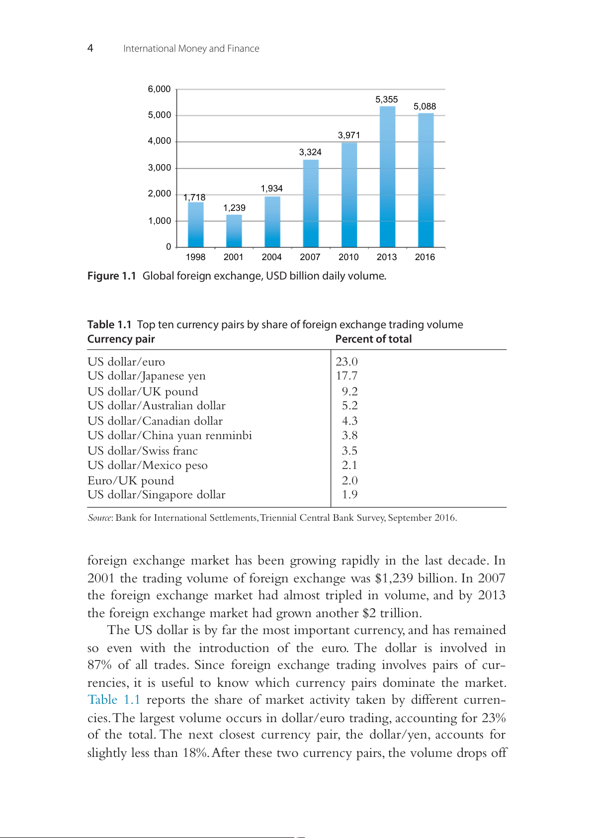
of trading volume around the world and in the 2016 survey the average
amount of currency traded each business day was $5,088 billion. Thus the
foreign exchange market is an enormous market. Fig. 1.1 shows that the © 201 7 Elsevier Inc.
International Money and Finance. All rights reserved. 3 4
International Money and Finance 6,000 5,355 5,088 5,000 3,971 4,000 3,324 3,000 1,934 2,000 1,718 1,239 1,000 0 1998 2001 2004 2007 2010 2013 2016
Figure 1.1 Global foreign exchange, USD billion daily volume.
Table 1.1 Top ten currency pairs by share of foreign exchange trading volume Currency pair Percent of total US dollar/euro 23.0 US dollar/Japanese yen 17.7 US dollar/UK pound 9.2 US dollar/Australian dollar 5.2 US dollar/Canadian dollar 4.3 US dollar/China yuan renminbi 3.8 US dollar/Swiss franc 3.5 US dollar/Mexico peso 2.1 Euro/UK pound 2.0 US dollar/Singapore dollar 1.9
Source: Bank for International Settlements, Triennial Central Bank Survey, September 2016.
foreign exchange market has been growing rapidly in the last decade. In
2001 the trading volume of foreign exchange was $1,239 billion. In 2007
the foreign exchange market had almost tripled in volume, and by 2013
the foreign exchange market had grown another $2 trillion.
The US dollar is by far the most important currency, and has remained
so even with the introduction of the euro. The dollar is involved in
87% of all trades. Since foreign exchange trading involves pairs of cur-
rencies, it is useful to know which currency pairs dominate the market.
Table 1.1 reports the share of market activity taken by different curren-
cies. The largest volume occurs in dollar/euro trading, accounting for 23%
of the total. The next closest currency pair, the dollar/yen, accounts for
slightly less than 18%. After these two currency pairs, the volume drops off The Foreign Exchange Market 5
dramatically. For example, the dollar/UK pound is roughly half as much
foreign currency trading as the dollar/yen. The US dollar is represented in
nine of the top ten currency pairs. Thus, the currency markets are domi- nated by dollar trading.
GEOGRAPHIC FOREIGN EXCHANGE RATE ACTIVITY
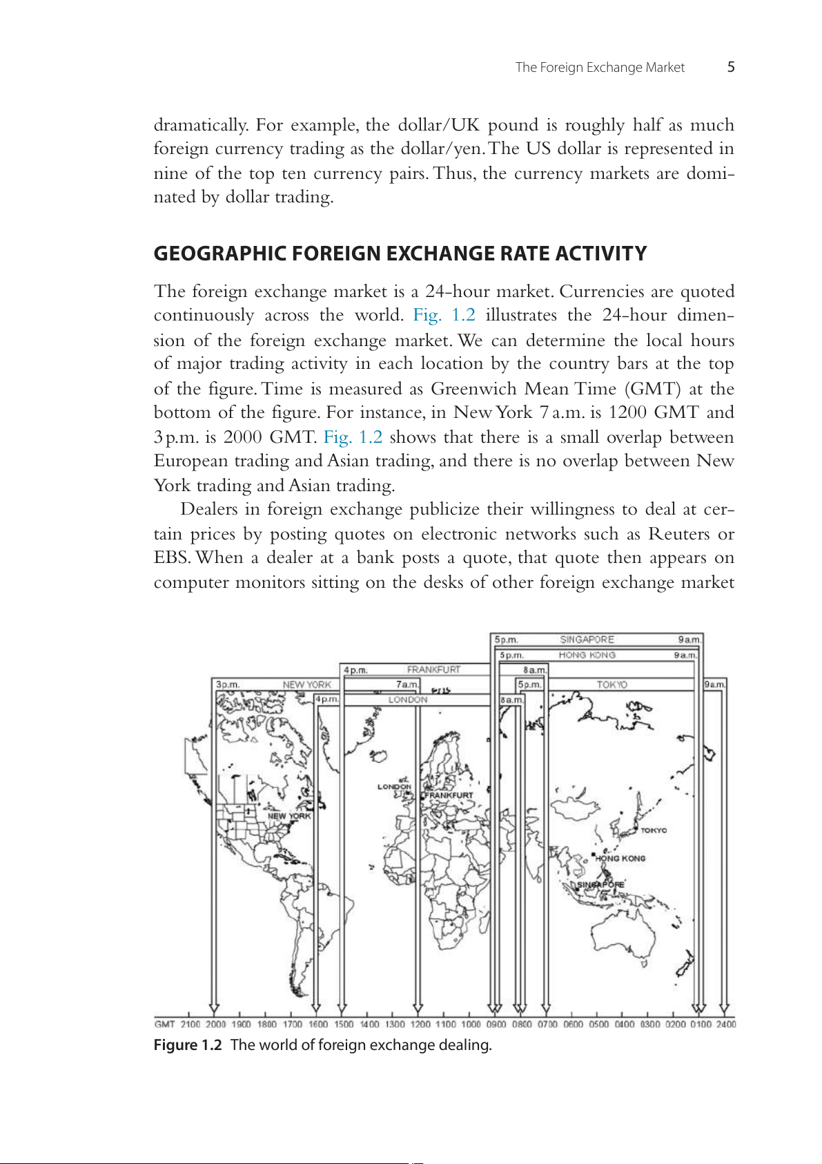
The foreign exchange market is a 24-hour market. Currencies are quoted
continuously across the world. Fig. 1.2 illustrates the 24-hour dimen-
sion of the foreign exchange market. We can determine the local hours
of major trading activity in each location by the country bars at the top
of the figure. Time is measured as Greenwich Mean Time (GMT) at the
bottom of the figure. For instance, in New York 7 a.m. is 1200 GMT and
3 p.m. is 2000 GMT. Fig. 1.2 shows that there is a small overlap between
European trading and Asian trading, and there is no overlap between New
York trading and Asian trading.
Dealers in foreign exchange publicize their willingness to deal at cer-
tain prices by posting quotes on electronic networks such as Reuters or
EBS. When a dealer at a bank posts a quote, that quote then appears on
computer monitors sitting on the desks of other foreign exchange market
Figure 1.2 The world of foreign exchange dealing. 6
International Money and Finance
participants worldwide. This posted quote is like an advertisement, tell-
ing the rest of the market the prices at which the quoting dealer is ready
to deal. In addition to the electronic trading venues, there is still bilateral
direct-dealing in the market where one person speaks with a bank dealer
to arrange a trade. These bilateral transactions and the quantities and prices
that are transacted are proprietary information and are known only by the
two participants in a transaction. The quotes on the electronic trading net-
works are the best publicly available information on the current prices in the market.
In terms of the geographic pattern of foreign exchange trading, a small
number of locations account for the majority of trading. Table 1.2 reports
the average daily volume of foreign exchange trading in different coun-
tries. The United Kingdom and the United States account for more than
half of the total world trading. The United Kingdom has long been the
leader in foreign exchange trading. In 2016, it accounted for just over 37%
of total world trading volume. While it is true that foreign exchange trad-
ing is a round-the-clock business, with trading taking place somewhere in
the world at any point in time, the peak activity occurs during business
hours in London, New York, and Tokyo.
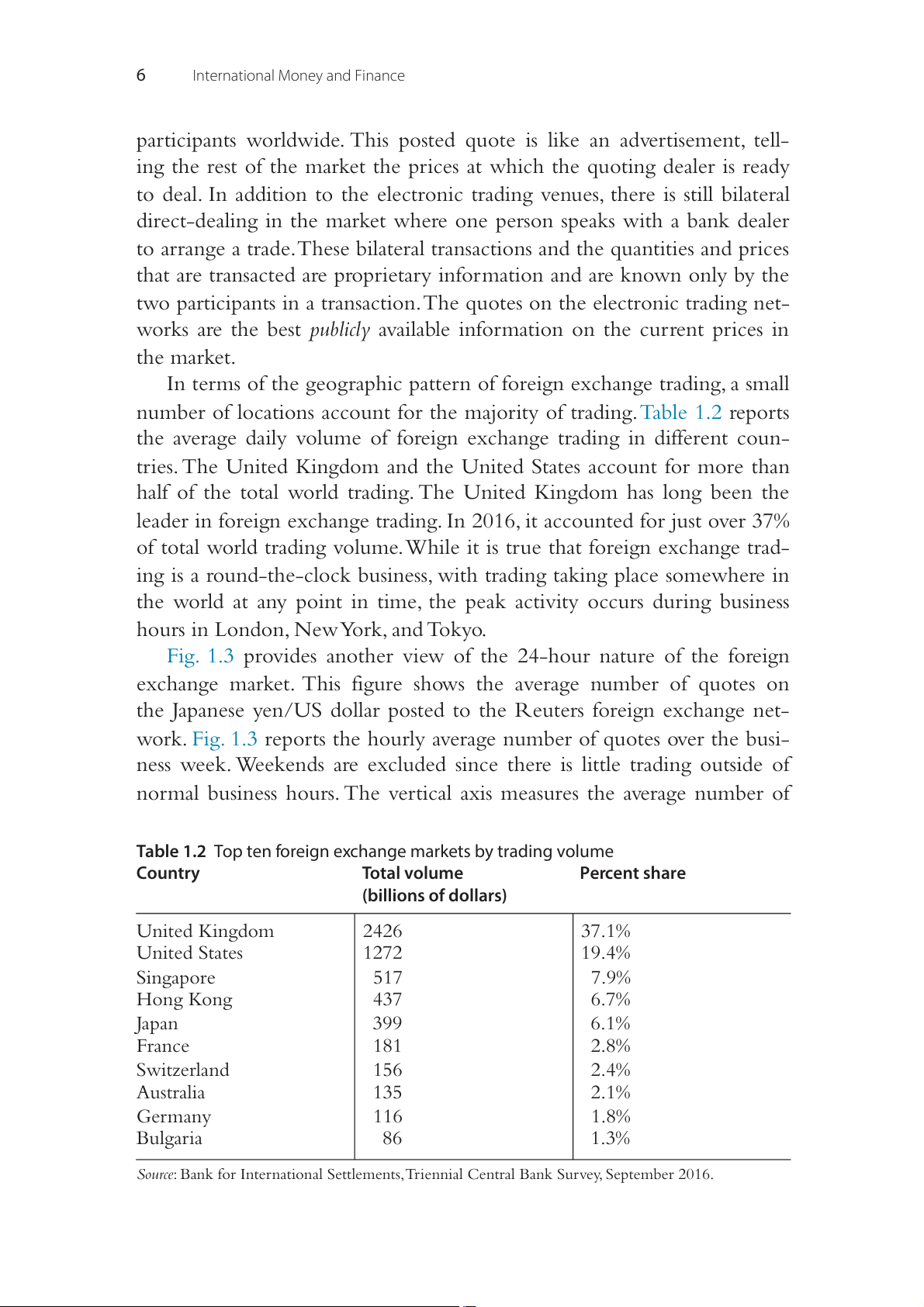
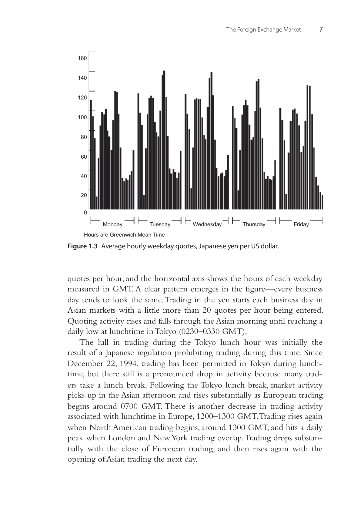
Fig. 1.3 provides another view of the 24-hour nature of the foreign
exchange market. This figure shows the average number of quotes on
the Japanese yen/US dollar posted to the Reuters foreign exchange net-
work. Fig. 1.3 reports the hourly average number of quotes over the busi-
ness week. Weekends are excluded since there is little trading outside of
normal business hours. The vertical axis measures the average number of
Table 1.2 Top ten foreign exchange markets by trading volume Country Total volume Percent share (billions of dollars) United Kingdom 2426 37.1% United States 1272 19.4% Singapore 517 7.9% Hong Kong 437 6.7% Japan 399 6.1% France 181 2.8% Switzerland 156 2.4% Australia 135 2.1% Germany 116 1.8% Bulgaria 86 1.3%
Source: Bank for International Settlements, Triennial Central Bank Survey, September 2016. The Foreign Exchange Market 7 160 140 120 r u o 100 r h e p s te 80 o u Q 60 40 20
0 0 1 2 3 4 5 6 7 8 9 0 1 2 3 4 5 6 7 8 9 0 1 2 3 0 1 2 3 4 5 6 7 8 9 0 1 2 3 0 1 2 3 4 5 6 7 8 9 0 1 2 3 0 1 2 3 4 5 6 7 8 9 0 1 2 3 0 1 2 3 4 5 6 7 8 9 0 1 2 3 1 1 1 1 1 1 1 1 1 1 2 2 2 2 0 1 2 3 4 5 6 7 8 9 1 1 1 1 1 1 1 1 1 1 2 2 2 2 0 1 2 3 4 5 6 7 8 9 1 1 1 1 1 1 1 1 1 1 2 2 2 2 0 1 2 3 4 5 6 7 8 9 1 1 1 1 1 1 1 1 1 1 2 2 2 2 0 1 2 3 4 5 6 7 8 9 1 1 1 1 1 1 1 1 1 1 2 2 2 2 Monday Tuesday Wednesday Thursday Friday Hours are Greenwich Mean Time
Figure 1.3 Average hourly weekday quotes, Japanese yen per US dollar.
quotes per hour, and the horizontal axis shows the hours of each weekday
measured in GMT. A clear pattern emerges in the figure—every business
day tends to look the same. Trading in the yen starts each business day in
Asian markets with a little more than 20 quotes per hour being entered.
Quoting activity rises and falls through the Asian morning until reaching a
daily low at lunchtime in Tokyo (0230–0330 GMT).
The lull in trading during the Tokyo lunch hour was initially the
result of a Japanese regulation prohibiting trading during this time. Since
December 22, 1994, trading has been permitted in Tokyo during lunch-
time, but there still is a pronounced drop in activity because many trad-
ers take a lunch break. Following the Tokyo lunch break, market activity
picks up in the Asian afternoon and rises substantially as European trading
begins around 0700 GMT. There is another decrease in trading activity
associated with lunchtime in Europe, 1200–1300 GMT. Trading rises again
when North American trading begins, around 1300 GMT, and hits a daily
peak when London and New York trading overlap. Trading drops substan-
tially with the close of European trading, and then rises again with the
opening of Asian trading the next day. 8
International Money and Finance
Note that every weekday has this same pattern, as the pace of the
activity in the foreign exchange market follows the opening and closing of
business hours around the world. While it is true that the foreign exchange
market is a 24-hour market with continuous trading possible, the amount
of trading follows predictable patterns. This is not to say that there are not
days that differ substantially from this average daily number of quotes. If
some surprising event occurs that stimulates trading, some days may have a
much different pattern. Later in the text we consider the determinants of
exchange rates and study what sorts of news would be especially relevant
to the foreign exchange market. SPOT EXCHANGE RATES
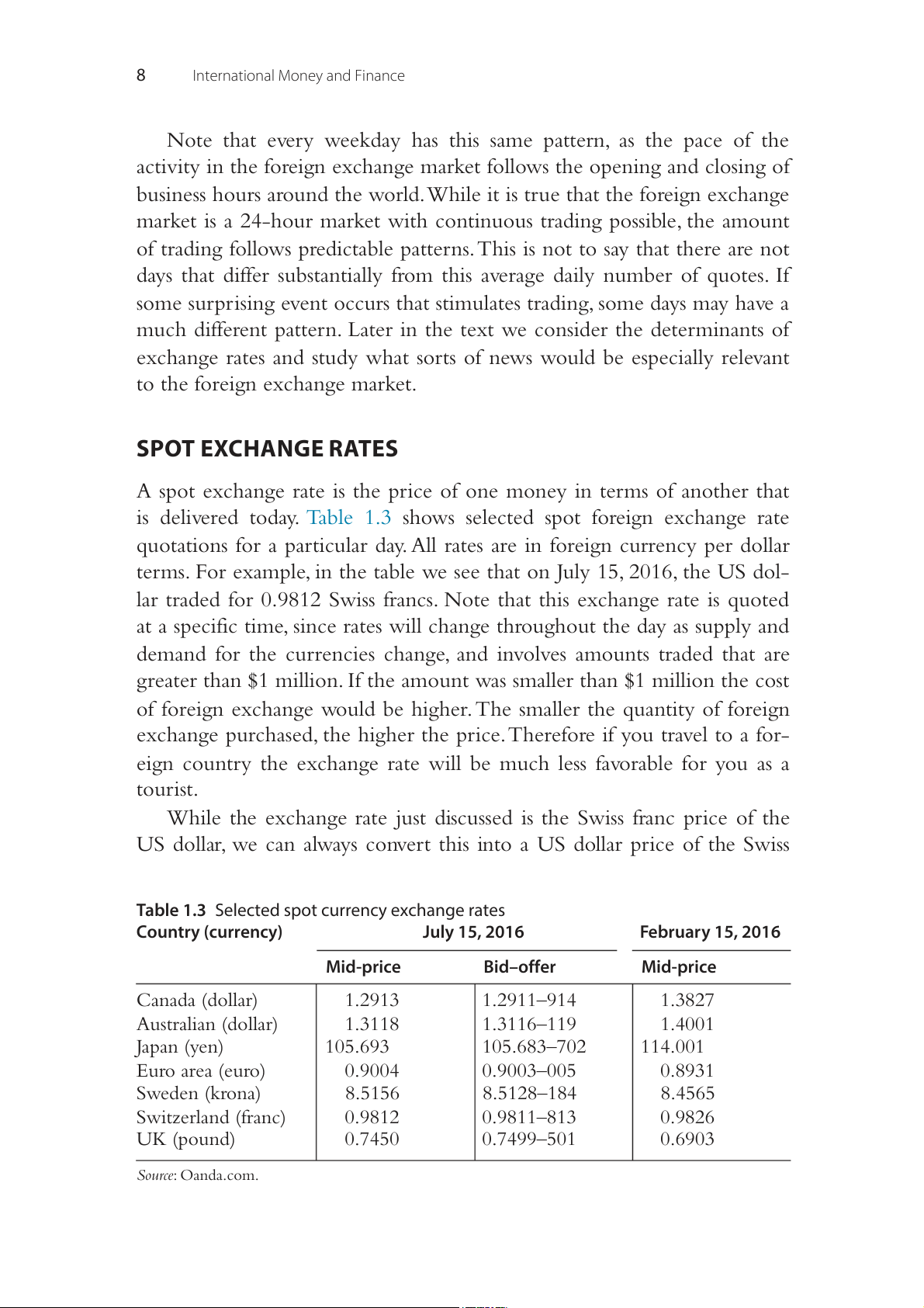
A spot exchange rate is the price of one money in terms of another that
is delivered today. Table 1.3 shows selected spot foreign exchange rate
quotations for a particular day. All rates are in foreign currency per dollar
terms. For example, in the table we see that on July 15, 2016, the US dol-
lar traded for 0.9812 Swiss francs. Note that this exchange rate is quoted
at a specific time, since rates will change throughout the day as supply and
demand for the currencies change, and involves amounts traded that are
greater than $1 million. If the amount was smaller than $1 million the cost
of foreign exchange would be higher. The smaller the quantity of foreign
exchange purchased, the higher the price. Therefore if you travel to a for-
eign country the exchange rate will be much less favorable for you as a tourist.
While the exchange rate just discussed is the Swiss franc price of the
US dollar, we can always convert this into a US dollar price of the Swiss
Table 1.3 Selected spot currency exchange rates Country (currency) July 15, 2016 February 15, 2016 Mid-price Bid–offer Mid-price Canada (dollar) 1.2913 1.2911–914 1.3827 Australian (dollar) 1.3118 1.3116–119 1.4001 Japan (yen) 105.693 105.683–702 114.001 Euro area (euro) 0.9004 0.9003–005 0.8931 Sweden (krona) 8.5156 8.5128–184 8.4565 Switzerland (franc) 0.9812 0.9811–813 0.9826 UK (pound) 0.7450 0.7499–501 0.6903 Source: Oanda.com. The Foreign Exchange Market 9
franc by taking the reciprocal of the exchange rate, or 1/exchange rate, For
instance, the exchange rate of 0.9812 Swiss francs per dollar is converted
into dollars per Swiss franc by calculating the reciprocal: 1/0.9812 =
1.019. It will always be true that when we know the Swiss franc price per
dollar (SF/$), we can find the dollar price per Swiss franc by taking the reciprocal 1/(SF/$) = ($/SF).
Note that the exchange rate quotes in the first column in Table 1.3 are
mid-price rates. For convenience we often talk about the spot rate as if it
is one rate. Often this rate is the mid-price rate. However, the spot rate
always involves two rates. Banks bid (buy) foreign exchange at lower rates
than they offer (sell), and the difference between the selling and buying rates
is called the spread. The mid-price is the average of the buying and selling
rates. Table 1.3 lists the spreads for the currencies in the second column.
The bid/offer prices is quoted so that one can see the bid (buy) price, and
one can find the offer (sell) price by dropping the last three digits of the
buy quote and replacing them with the second number. For example, the
Swiss franc bid–offer price is 0.9811 8
– 13. Thus, the bank is willing to buy
dollars for Swiss francs at 0.9811, and sell dollars at 0.9813 Swiss francs.
The spread (the bank’s profit) between the buy and sell rates is very small.
The spread for the Swiss franc can be measured in percentage terms
as the (ask-bid)/mid-price. Using the information in Table 1.3, we can
compute the spread in percentage terms as [(0.9813-0.9811)/0.9812 =
0.0002], or 2/100 of 1%. This spread is indicative of how small the normal
spread is in the market for major traded currencies. The existing spread in
any currency will vary according to the individual currency trader, the cur-
rency being traded, and the trading bank’s overall view of conditions in the
foreign exchange market. The spread quoted will tend to increase for more
thinly traded currencies (i.e., currencies that do not generate a large volume
of trading) or when the bank perceives that the risks associated with trading
in a currency at a particular time are rising.
Let us look at an example of using the buy and sell rates. If you were a
US importer buying watches from Switzerland at the dollar price of $10
million, a bank would sell $10 million worth of Swiss francs to you for
0.9811 Swiss francs per dollar. Note that Table 1.3 shows what banks are
willing to bid and offer when buying or selling dollars for Swiss franc.
We want to sell our dollars for Swiss franc so we need to use the bid
rate for the bank in Table 1.3. You would receive SF9,811,000 to settle the
account with the Swiss exporter.
$10,000,000*0.9811 SF/$ = SF9,811,000 10
International Money and Finance
Table 1.4 International currency symbols Country Currency Symbol ISOcode Australia Dollar A$ AUD Austria Euro € EUR Belgium Euro € EUR Canada Dollar C$ CAD Denmark Krone DKr DKK Finland Euro € EUR France Euro € EUR Germany Euro € EUR Greece Euro € EUR India Rupee ₹ INR Iran Rial RI IRR Italy Euro € EUR Japan Yen ¥ JPY Kuwait Dinar KD KWD Mexico Peso Ps MXN Netherlands Euro € EUR Norway Krone NKr NOK Saudi Arabia Riyal SR SAR Singapore Dollar S$ SGD South Africa Rand R ZAR Spain Euro € EUR Sweden Krona SKr SEK Switzerland Franc SF CHF United Kingdom Pound £ GBP United States Dollar $ USD
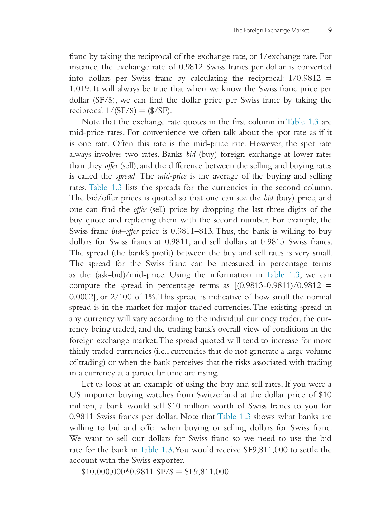
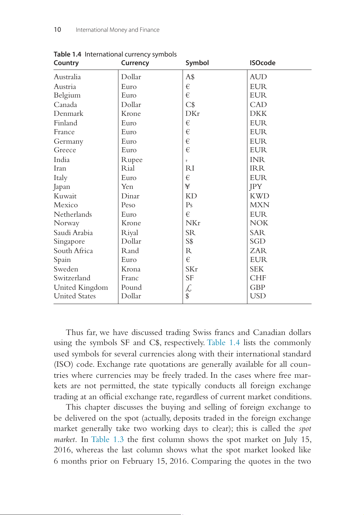
Thus far, we have discussed trading Swiss francs and Canadian dollars
using the symbols SF and C$, respectively. Table 1.4 lists the commonly
used symbols for several currencies along with their international standard
(ISO) code. Exchange rate quotations are generally available for all coun-
tries where currencies may be freely traded. In the cases where free mar-
kets are not permitted, the state typically conducts all foreign exchange
trading at an official exchange rate, regardless of current market conditions.
This chapter discusses the buying and selling of foreign exchange to
be delivered on the spot (actually, deposits traded in the foreign exchange
market generally take two working days to clear); this is called the spot
market. In Table 1.3 the first column shows the spot market on July 15,
2016, whereas the last column shows what the spot market looked like
6 months prior on February 15, 2016. Comparing the quotes in the two The Foreign Exchange Market 11
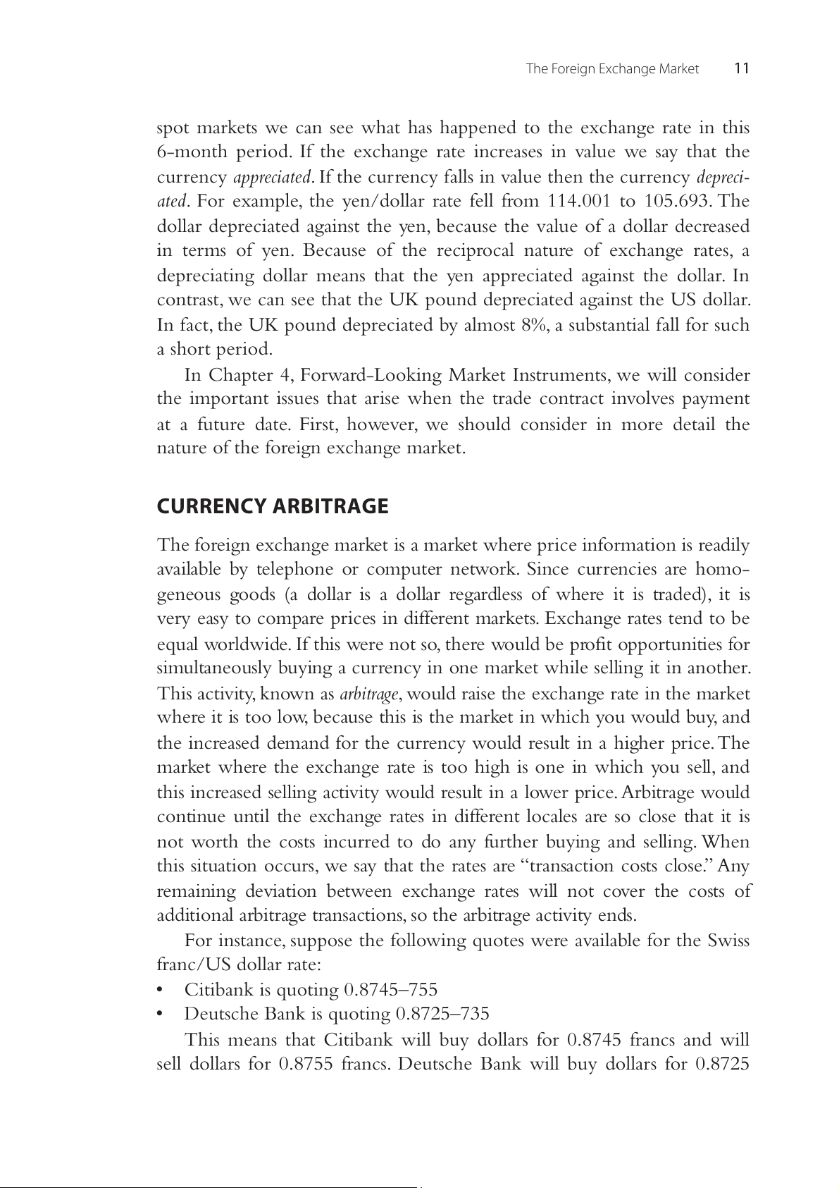
spot markets we can see what has happened to the exchange rate in this
6-month period. If the exchange rate increases in value we say that the
currency appreciated. If the currency falls in value then the currency depreci-
ated. For example, the yen/dollar rate fell from 114.001 to 105.693. The
dollar depreciated against the yen, because the value of a dollar decreased
in terms of yen. Because of the reciprocal nature of exchange rates, a
depreciating dollar means that the yen appreciated against the dollar. In
contrast, we can see that the UK pound depreciated against the US dollar.
In fact, the UK pound depreciated by almost 8%, a substantial fall for such a short period.
In Chapter4, Forward-Looking Market Instruments, we will consider
the important issues that arise when the trade contract involves payment
at a future date. First, however, we should consider in more detail the
nature of the foreign exchange market. CURRENCY ARBITRAGE
The foreign exchange market is a market where price information is readily
available by telephone or computer network. Since currencies are homo-
geneous goods (a dollar is a dollar regardless of where it is traded), it is
very easy to compare prices in different markets. Exchange rates tend to be
equal worldwide. If this were not so, there would be profit opportunities for
simultaneously buying a currency in one market while selling it in another.
This activity, known as arbitrage, would raise the exchange rate in the market
where it is too low, because this is the market in which you would buy, and
the increased demand for the currency would result in a higher price. The
market where the exchange rate is too high is one in which you sell, and
this increased selling activity would result in a lower price. Arbitrage would
continue until the exchange rates in different locales are so close that it is
not worth the costs incurred to do any further buying and selling. When
this situation occurs, we say that the rates are “transaction costs close.” Any
remaining deviation between exchange rates will not cover the costs of
additional arbitrage transactions, so the arbitrage activity ends.
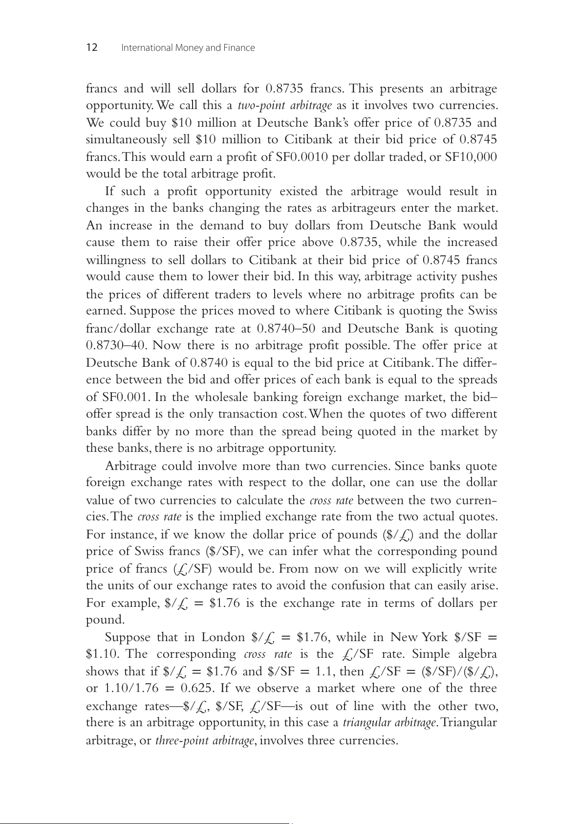
For instance, suppose the following quotes were available for the Swiss franc/US dollar rate: ●
Citibank is quoting 0.8745–755 ●
Deutsche Bank is quoting 0.8725–735
This means that Citibank will buy dollars for 0.8745 francs and will
sell dollars for 0.8755 francs. Deutsche Bank will buy dollars for 0.8725 12
International Money and Finance
francs and will sell dollars for 0.8735 francs. This presents an arbitrage
opportunity. We call this a two-point arbitrage as it involves two currencies.
We could buy $10 million at Deutsche Bank’s offer price of 0.8735 and
simultaneously sell $10 million to Citibank at their bid price of 0.8745
francs. This would earn a profit of SF0.0010 per dollar traded, or SF10,000
would be the total arbitrage profit.
If such a profit opportunity existed the arbitrage would result in
changes in the banks changing the rates as arbitrageurs enter the market.
An increase in the demand to buy dollars from Deutsche Bank would
cause them to raise their offer price above 0.8735, while the increased
willingness to sell dollars to Citibank at their bid price of 0.8745 francs
would cause them to lower their bid. In this way, arbitrage activity pushes
the prices of different traders to levels where no arbitrage profits can be
earned. Suppose the prices moved to where Citibank is quoting the Swiss
franc/dollar exchange rate at 0.8740–50 and Deutsche Bank is quoting
0.8730–40. Now there is no arbitrage profit possible. The offer price at
Deutsche Bank of 0.8740 is equal to the bid price at Citibank. The differ-
ence between the bid and offer prices of each bank is equal to the spreads
of SF0.001. In the wholesale banking foreign exchange market, the bid–
offer spread is the only transaction cost. When the quotes of two different
banks differ by no more than the spread being quoted in the market by
these banks, there is no arbitrage opportunity.
Arbitrage could involve more than two currencies. Since banks quote
foreign exchange rates with respect to the dollar, one can use the dollar
value of two currencies to calculate the cross rate between the two curren-
cies. The cross rate is the implied exchange rate from the two actual quotes.
For instance, if we know the dollar price of pounds ($/£) and the dollar
price of Swiss francs ($/SF), we can infer what the corresponding pound
price of francs (£/SF) would be. From now on we will explicitly write
the units of our exchange rates to avoid the confusion that can easily arise.
For example, $/£ = $1.76 is the exchange rate in terms of dollars per pound.
Suppose that in London $/£ = $1.76, while in New York $/SF =
$1.10. The corresponding cross rate is the £/SF rate. Simple algebra
shows that if $/£ = $1.76 and $/SF = 1.1, then £/SF = ($/SF)/($/£),
or 1.10/1.76 = 0.625. If we observe a market where one of the three
exchange rates—$/£, $/SF, £/SF—is out of line with the other two,
there is an arbitrage opportunity, in this case a triangular arbitrage. Triangular
arbitrage, or three-point arbitrage, involves three currencies. The Foreign Exchange Market 13
Table 1.5 Triangular arbitrage Location $/SF $/£ £/SF New York 1.100 1.600 – London – 1.600 0.625 Geneva 1.100 – 0.625
To simplify the analysis of arbitrage involving three currencies, let us
ignore the bid–offer spread and assume that we can either buy or sell at one
price. Suppose that in Geneva, Switzerland the exchange rate is £/SF =
0.625, while in New York $/SF = 1.100, and in London $/£ = $1.600, as
shown in Table 1.5. Examining Table 1.5 it appears to have no possible arbi-
trage opportunity, but astute traders in the foreign exchange market would
observe a discrepancy when they check the cross rates. Computing the
implicit cross rate for New York, the arbitrageur finds the implicit cross rate
to be £/SF = ($/SF)/($/£), or 1.100/1.600 = 0.6875. Thus the cost of SF
is high in New York, and the cost of £ is low.
Assume that a trader starts in New York with 1 million dollars. The
trader should buy £ in New York. Selling $1 million in New York (or
London) the trader receives £625,000 ($1 million divided by $/£ =
$1.60). The pounds then are used to buy Swiss francs at £/SF = 0.625
(in either London or Geneva), so that £625,000 = SF1 million. The SF1
million would be used in New York to buy dollars at $/SF = $1.10, so
that SF1 million = $1,100,000. Thus the initial $1 million could be turned
into $1,100,000, with the triangular arbitrage action earning the trader
$100,000 (costs associated with the transaction should be deducted to
arrive at the true arbitrage profit).
As in the case of the two-currency arbitrage covered earlier, a valu-
able product of this arbitrage activity is the return of the exchange rates
to internationally consistent levels. If the initial discrepancy was that the
dollar price of pounds was too low in London, the selling of dollars for
pounds in London by the arbitrageurs will make pounds more expensive,
raising the price from $/£ = $1.60. Note that if the pound cost increases
to $/£ = $1.76 then there is no arbitrage possible. However, the pound
exchange rate is unlikely to increase that much because the activity in the
other markets would tend to raise the pound price of francs and lower
the dollar price of francs, so that a dollar price of pounds somewhere
between $1.60 and $1.76 would be the new equilibrium among the three currencies. 14
International Money and Finance
Since there is active trading between the dollar and other curren-
cies, we can look to any two exchange rates involving dollars to infer the
cross rates. So even if there is limited direct trading between, for instance,
Mexican pesos and yen, by using pesos/$ and $/¥, we can find the implied
pesos/¥ rate. Since transaction costs are higher for lightly traded curren-
cies, the depth of foreign exchange trading that involves dollars often
makes it cheaper to go through dollars to get from some currency X to another currency Y when X and
Y are not widely traded. Thus, if a busi-
ness firm in small country X wants to buy currency Y to pay for merchan-
dise imports from small country Y, it may well be cheaper to sell X for
dollars and then use dollars to buy Y rather than try to trade currency X for currency Y directly.
SHORT-TERM FOREIGN EXCHANGE RATE MOVEMENTS
Understanding the “market microstructure” allows us to explain the evo-
lution of the foreign exchange market in an intradaily sense, in which
foreign exchange traders adjust their bid and offer quotes throughout the business day.
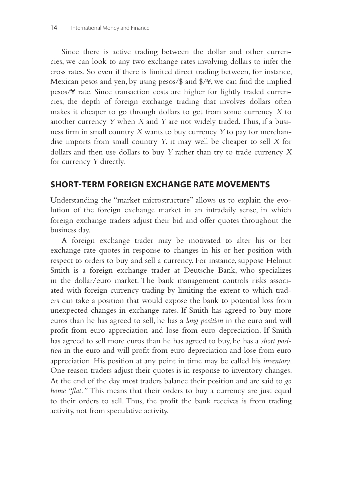
A foreign exchange trader may be motivated to alter his or her
exchange rate quotes in response to changes in his or her position with
respect to orders to buy and sell a currency. For instance, suppose Helmut
Smith is a foreign exchange trader at Deutsche Bank, who specializes
in the dollar/euro market. The bank management controls risks associ-
ated with foreign currency trading by limiting the extent to which trad-
ers can take a position that would expose the bank to potential loss from
unexpected changes in exchange rates. If Smith has agreed to buy more
euros than he has agreed to sell, he has a long position in the euro and will
profit from euro appreciation and lose from euro depreciation. If Smith
has agreed to sell more euros than he has agreed to buy, he has a short posi-
tion in the euro and will profit from euro depreciation and lose from euro
appreciation. His position at any point in time may be called his inventory.
One reason traders adjust their quotes is in response to inventory changes.
At the end of the day most traders balance their position and are said to go
home “flat.” This means that their orders to buy a currency are just equal
to their orders to sell. Thus, the profit the bank receives is from trading
activity, not from speculative activity. The Foreign Exchange Market 15
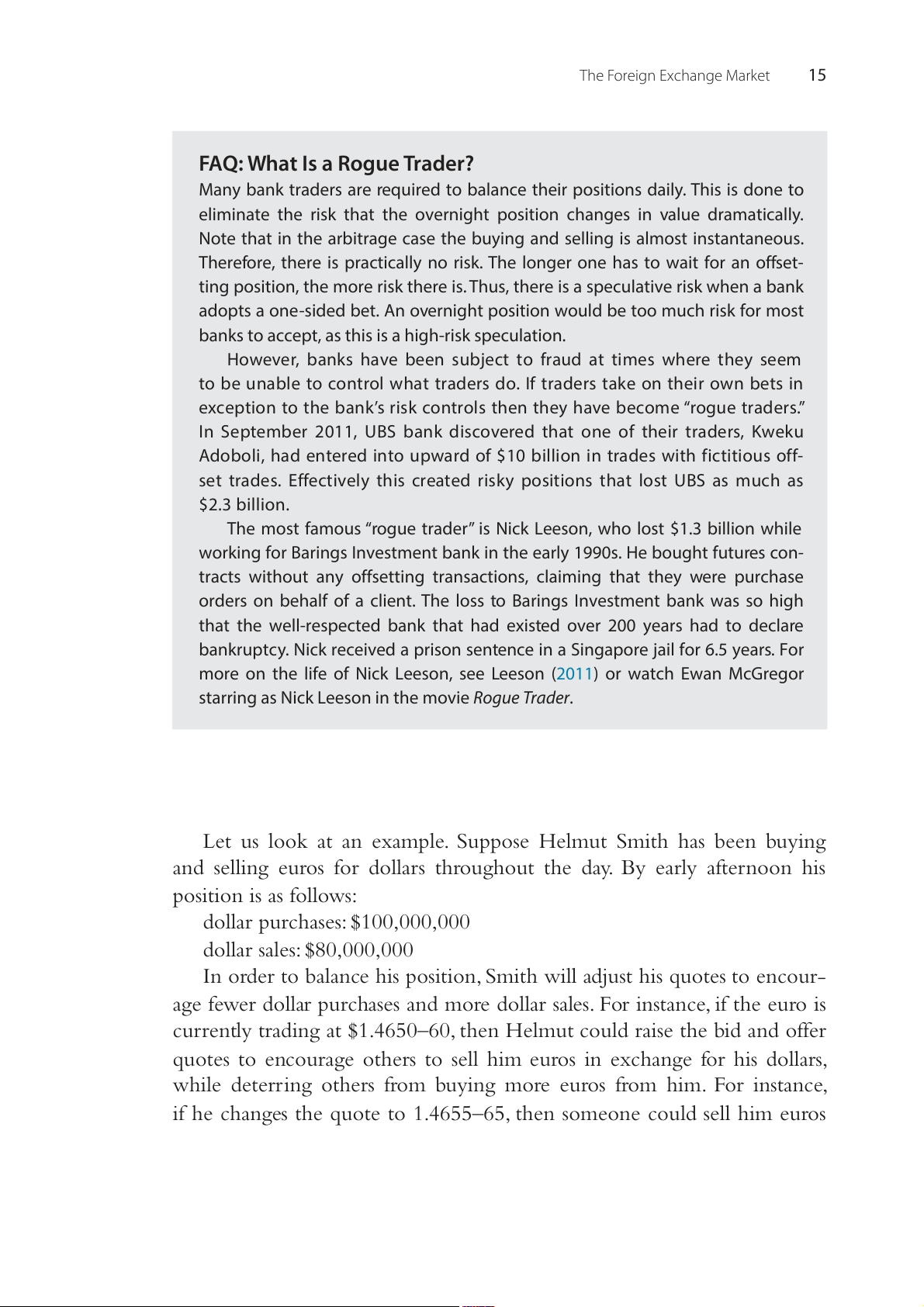
FAQ: What Is a Rogue Trader?
Many bank traders are required to balance their positions daily. This is done to
eliminate the risk that the overnight position changes in value dramatically.
Note that in the arbitrage case the buying and selling is almost instantaneous.
Therefore, there is practically no risk. The longer one has to wait for an offset-
ting position, the more risk there is. Thus, there is a speculative risk when a bank
adopts a one-sided bet. An overnight position would be too much risk for most
banks to accept, as this is a high-risk speculation.
However, banks have been subject to fraud at times where they seem
to be unable to control what traders do. If traders take on their own bets in
exception to the bank’s risk controls then they have become “rogue traders.”
In September 2011, UBS bank discovered that one of their traders, Kweku
Adoboli, had entered into upward of $10 billion in trades with fictitious off-
set trades. Effectively this created risky positions that lost UBS as much as $2.3 billion.
The most famous “rogue trader” is Nick Leeson, who lost $1.3 billion while
working for Barings Investment bank in the early 1990s. He bought futures con-
tracts without any offsetting transactions, claiming that they were purchase
orders on behalf of a client. The loss to Barings Investment bank was so high
that the well-respected bank that had existed over 200 years had to declare
bankruptcy. Nick received a prison sentence in a Singapore jail for 6.5 years. For
more on the life of Nick Leeson, see Leeson (2011) or watch Ewan McGregor
starring as Nick Leeson in the movie Rogue Trader.
Let us look at an example. Suppose Helmut Smith has been buying
and selling euros for dollars throughout the day. By early afternoon his position is as follows: dollar purchases: $100,000,000 dollar sales: $80,000,000
In order to balance his position, Smith will adjust his quotes to encour-
age fewer dollar purchases and more dollar sales. For instance, if the euro is
currently trading at $1.4650–60, then Helmut could raise the bid and offer
quotes to encourage others to sell him euros in exchange for his dollars,
while deterring others from buying more euros from him. For instance,
if he changes the quote to 1.4655–65, then someone could sell him euros 16
International Money and Finance
(or buy his dollars) for $1.4655 per euro. Since he has raised the dollar
price of a euro, he will receive more interest from people wanting to sell
him euros in exchange for his dollars. When Helmut buys euros from
other traders, he is selling them dollars, and this helps to balance his inven-
tory and reduce his long position in the dollar. At the same time Helmut
has raised the sell rate of euros to $1.4665. This discourages other traders
from buying more euros from Helmut (giving him dollars as payments).
This inventory control effect on exchange rates can explain why trad-
ers may alter their quotes in the absence of any news about exchange rate fundamentals.
In addition to the inventory control effect, there is also an asymmet-
ric information effect, which causes exchange rates to change due to trad-
ers’ fears that they are quoting prices to someone who knows more about
current market conditions than they do. Even without news regarding the
fundamentals, information is being transmitted from one trader to another
through the act of trading. If Helmut posts a quote of 1.0250–260 and is
called by Ingrid Schultz at Citibank asking to buy $5 million of euros at
Helmut’s offer price of 1.0260, Helmut then must wonder whether Ingrid
knows something he doesn’t. Should Ingrid’s order to trade at Helmut’s
price be considered a signal that Helmut’s price is too low? What superior
information could Ingrid have? Every bank receives orders from nonbank
customers to buy and sell currency. Perhaps Ingrid knows that her bank
has just received a large order from Daimler Benz to sell dollars, and she is
selling dollars (and buying euros) in advance of the price increase that will
be caused by this nonbank order being filled by purchasing euros from other traders.
Helmut does not know why Ingrid is buying euros at his offer price,
but he protects himself from further euro sales to someone who may be
better informed than he is by raising his offer price. The bid price may be
left unchanged because the order was to buy his euros; in such a case the
spread increases, with the higher offer price due to the possibility of trad-
ing with a better-informed counterparty who wants him to sell euros.
The inventory control and asymmetric information effects can help
explain why exchange rates change throughout the day, even in the
absence of news regarding the fundamental determinants of exchange
rates. The act of trading generates price changes among risk-averse traders
who seek to manage their inventory positions to limit their exposure to
surprising exchange rate changes and limit the potential loss from trading
with better-informed individuals. The Foreign Exchange Market 17
LONG-TERM FOREIGN EXCHANGE MOVEMENTS
Thus far we have examined short-run movements in exchange rates. For
the most part we are interested in long-term movements in this book.
Since the exchange rate is the price of one money in terms of another,
changes in exchange rates affect the prices of goods and services traded
internationally. Therefore most of this book is concerned with why
exchange rates move and how we can avoid these effects. In this section
we will introduce a simple but powerful tool, called the trade flow model.
The trade flow model argues that the exchange rate responds to the
demand for traded goods by countries.
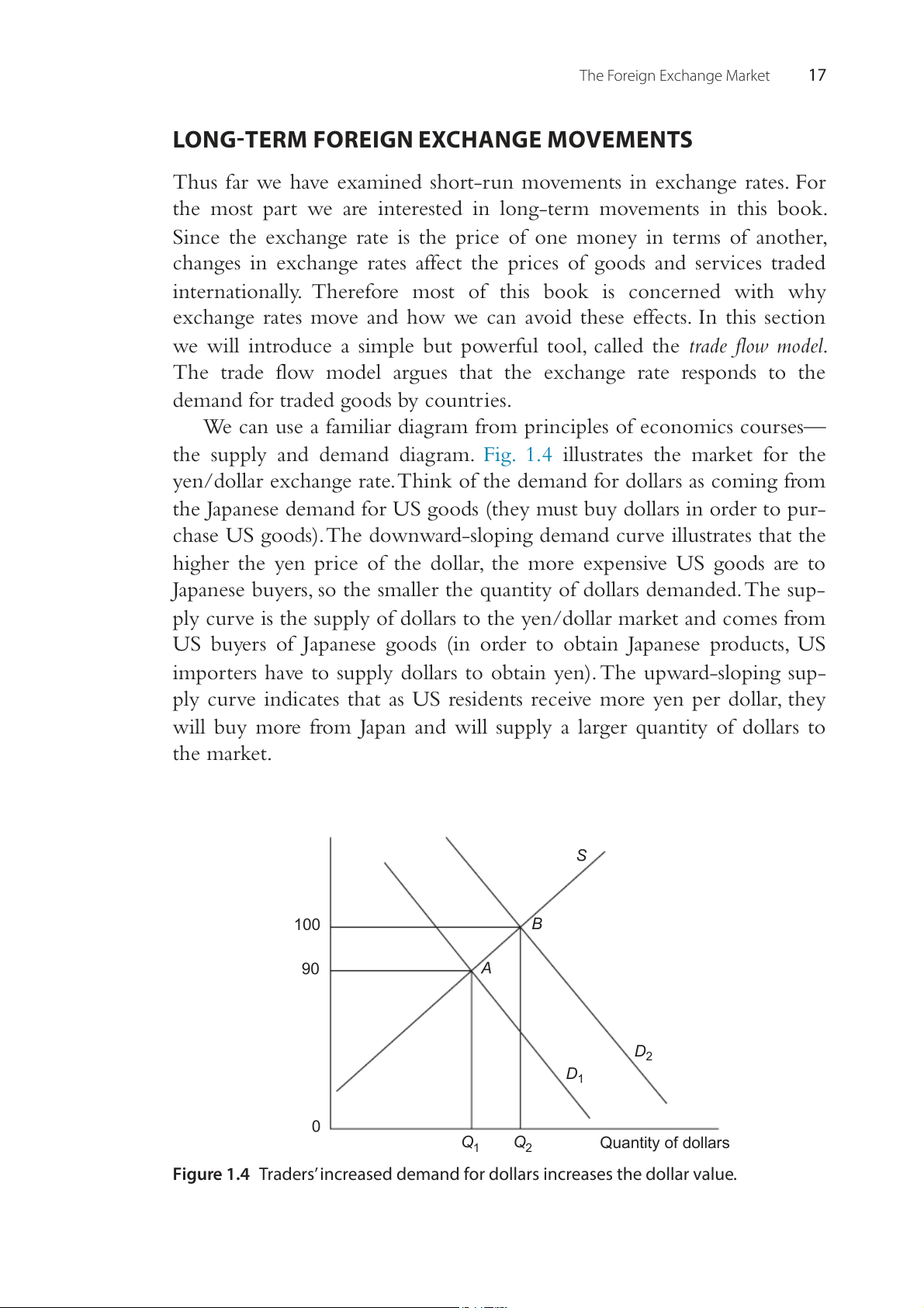
We can use a familiar diagram from principles of economics courses—
the supply and demand diagram. Fig. 1.4 illustrates the market for the
yen/dollar exchange rate. Think of the demand for dollars as coming from
the Japanese demand for US goods (they must buy dollars in order to pur-
chase US goods). The downward-sloping demand curve illustrates that the
higher the yen price of the dollar, the more expensive US goods are to
Japanese buyers, so the smaller the quantity of dollars demanded. The sup-
ply curve is the supply of dollars to the yen/dollar market and comes from
US buyers of Japanese goods (in order to obtain Japanese products, US
importers have to supply dollars to obtain yen). The upward-sloping sup-
ply curve indicates that as US residents receive more yen per dollar, they
will buy more from Japan and will supply a larger quantity of dollars to the market. S te ra 100 B e g n a 90 A xch r e lla o /d n D e 2 Y D1 0 Q Q Quantity of dollars 1 2
Figure 1.4 Traders’ increased demand for dollars increases the dollar value. 18
International Money and Finance
The initial equilibrium exchange rate is at point A, where the
exchange rate is 90 yen per dollar. Now suppose there is an increase in
Japanese demand for US products. This increases the demand for dollars
so that the demand curve shifts from D1 to D2. The equilibrium exchange
rate will now change to 100 yen per dollar at point B as the dollar appre-
ciates in value against the yen. This dollar appreciation makes Japanese goods cheaper to US buyers.
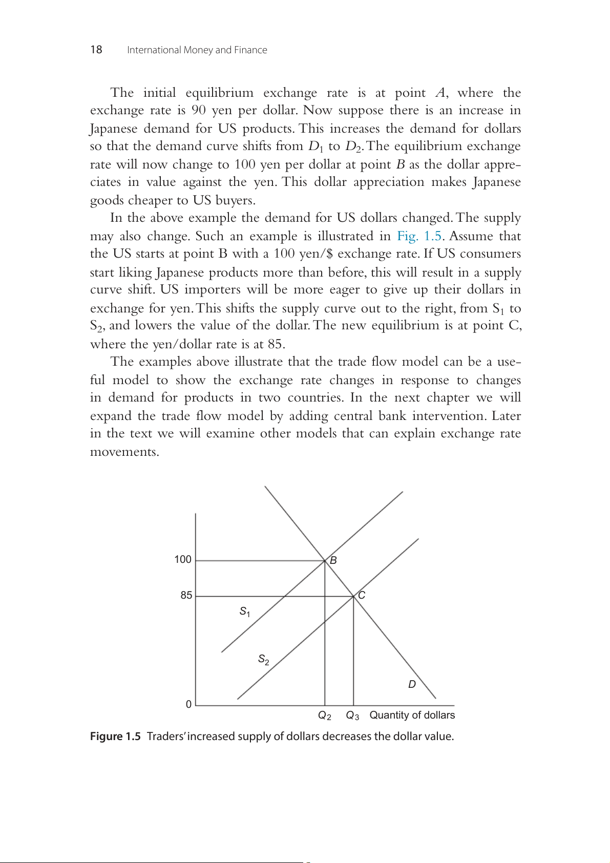
In the above example the demand for US dollars changed. The supply
may also change. Such an example is illustrated in Fig. 1.5. Assume that
the US starts at point B with a 100 yen/$ exchange rate. If US consumers
start liking Japanese products more than before, this will result in a supply
curve shift. US importers will be more eager to give up their dollars in
exchange for yen. This shifts the supply curve out to the right, from S1 to
S2, and lowers the value of the dollar. The new equilibrium is at point C,
where the yen/dollar rate is at 85.
The examples above illustrate that the trade flow model can be a use-
ful model to show the exchange rate changes in response to changes
in demand for products in two countries. In the next chapter we will
expand the trade flow model by adding central bank intervention. Later
in the text we will examine other models that can explain exchange rate movements. te 100 B ra e g n a 85 C xch S1 r e lla o /d n e S Y 2 D 0 Q 2 Q 3 Quantity of dollars
Figure 1.5 Traders’ increased supply of dollars decreases the dollar value. The Foreign Exchange Market 19 SUMMARY
1. The foreign exchange market is a global market where foreign cur-
rency deposits are traded. Trading in actual currency notes is generally
limited to tourism or illegal activities.
2. The dollar/euro currency pair dominates foreign exchange trading
volume, and the United Kingdom is the largest trading location.
3. A spot exchange rate is the price of a currency in terms of another
currency for current delivery. Banks buy (bid) foreign exchange at a
lower rate than they sell (offer), and the difference between the selling
and buying rates is called the spread.
4. Arbitrage realizes riskless profit from market disequilibrium by buying
a currency in one market and selling it in another. Arbitrage ensures
that exchange rates are transaction costs close in all markets.
5. The factors that explain why exchange rates vary so much in the short
run are inventory control and asymmetric information.
6. In the long run, economic factors (e.g., demand/supply of foreign
and domestic goods) affect the exchange rate movements. The trade
flow model is useful for discussing fundamental changes in the foreign exchange rate. EXERCISES
1. Suppose Nomura Bank quotes the ¥/$ exchange rate as 110.30–.40.
Assume you need ¥100,000. How much dollars do you need to pay
Nomura Bank to buy ¥100,000. Explain.
2. Compute the cross rate for the following quotes.
a. Compute the C$/€ using the following C$/$ = 1.5613, $/€ = 1.0008
b. Compute the £/¥ using the following ¥/$ = 124.84, $/£ = 1.5720
c. Compute the SF/C$ using the following SF/$ = 1.4706, C$/$ = 1.5613
3. Suppose Citibank quotes the ¥/$ exchange rate as 110.30–.40 and
Nomura Bank quotes 110.40–.50. Is there an arbitrage opportunity?
If so, explain how you would profit from these quotes. If not, explain why not. 20
International Money and Finance
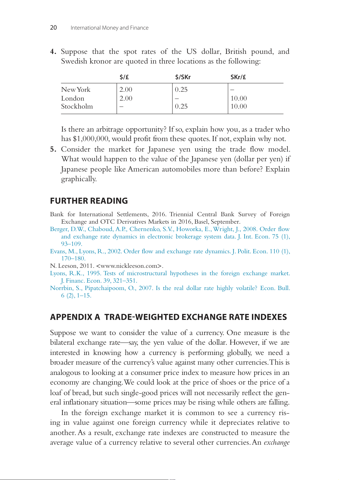
4. Suppose that the spot rates of the US dollar, British pound, and
Swedish kronor are quoted in three locations as the following: $/£ $/SKr SKr/£ New York 2.00 0.25 – London 2.00 – 10.00 Stockholm – 0.25 10.00
Is there an arbitrage opportunity? If so, explain how you, as a trader who
has $1,000,000, would profit from these quotes. If not, explain why not.
5. Consider the market for Japanese yen using the trade flow model.
What would happen to the value of the Japanese yen (dollar per yen) if
Japanese people like American automobiles more than before? Explain graphically. FURTHER READING
Bank for International Settlements, 2016. Triennial Central Bank Survey of Foreign
Exchange and OTC Derivatives Markets in 2016, Basel, September.
Berger, D.W., Chaboud, A.P., Chernenko, S.V., Howorka, E., Wright, J., 2008. Order flow
and exchange rate dynamics in electronic brokerage system data. J. Int. Econ. 75 (1), 93–109.
Evans, M., Lyons, R., 2002. Order flow and exchange rate dynamics. J. Polit. Econ. 110 (1), 170–180. N. Leeson, 2011. .
Lyons, R.K., 1995. Tests of microstructural hypotheses in the foreign exchange market.
J. Financ. Econ. 39, 321–351.
Norrbin, S., Pipatchaipoom, O., 2007. Is the real dollar rate highly volatile? Econ. Bull. 6 (2), 1–15.
APPENDIX A TRADE-WEIGHTED EXCHANGE RATE INDEXES
Suppose we want to consider the value of a currency. One measure is the
bilateral exchange rate—say, the yen value of the dollar. However, if we are
interested in knowing how a currency is performing globally, we need a
broader measure of the currency’s value against many other currencies. This is
analogous to looking at a consumer price index to measure how prices in an
economy are changing. We could look at the price of shoes or the price of a
loaf of bread, but such single-good prices will not necessarily reflect the gen-
eral inflationary situation—some prices may be rising while others are falling.
In the foreign exchange market it is common to see a currency ris-
ing in value against one foreign currency while it depreciates relative to
another. As a result, exchange rate indexes are constructed to measure the
average value of a currency relative to several other currencies. An exchange The Foreign Exchange Market 21
rate index is a weighted average of a currency’s value relative to other cur-
rencies, with the weights typically based on the importance of each cur-
rency to international trade. If we want to construct an exchange rate
index for the United States, we would include the currencies of the coun-
tries that are the major trading partners of the United States.
If half of US trade was with Canada and the other half was with
Mexico, then the percentage change in the trade-weighted dollar exchange
rate index would be found by multiplying the percentage change in both
the Canadian dollar/US dollar exchange rate and the Mexican peso/
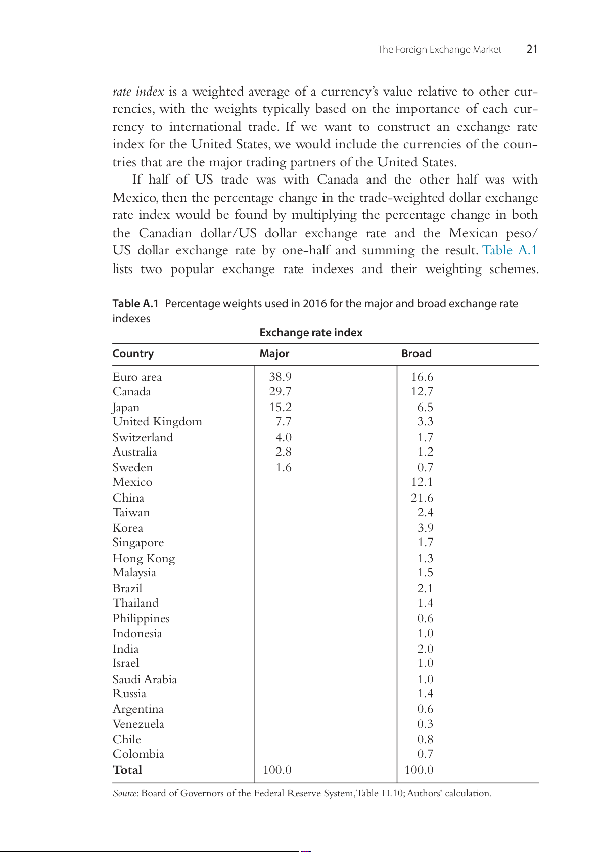
US dollar exchange rate by one-half and summing the result. Table A.1
lists two popular exchange rate indexes and their weighting schemes.
Table A.1 Percentage weights used in 2016 for the major and broad exchange rate indexes Exchange rate index Country Major Broad Euro area 38.9 16.6 Canada 29.7 12.7 Japan 15.2 6.5 United Kingdom 7.7 3.3 Switzerland 4.0 1.7 Australia 2.8 1.2 Sweden 1.6 0.7 Mexico 12.1 China 21.6 Taiwan 2.4 Korea 3.9 Singapore 1.7 Hong Kong 1.3 Malaysia 1.5 Brazil 2.1 Thailand 1.4 Philippines 0.6 Indonesia 1.0 India 2.0 Israel 1.0 Saudi Arabia 1.0 Russia 1.4 Argentina 0.6 Venezuela 0.3 Chile 0.8 Colombia 0.7 Total 100.0 100.0
Source: Board of Governors of the Federal Reserve System, Table H.10; Authors' calculation. 22
International Money and Finance 180 Broad currency index Major currency index 160 140 120 100 80 60 40 20 0 3 3 4 5 6 7 8 8 9 0 1 2 3 3 4 5 6 7 8 8 9 0 1 2 3 3 4 5 6 7 8 8 9 0 1 2 3 3 4 5 6 7 8 8 9 0 1 2 3 3 4 5 7 7 7 7 7 7 7 7 7 8 8 8 8 8 8 8 8 8 8 8 8 9 9 9 9 9 9 9 9 9 9 9 9 0 0 0 0 0 0 0 0 0 0 0 0 1 1 1 1 1 1 1 9 9 9 9 9 9 9 9 9 9 9 9 9 9 9 9 9 9 9 9 9 9 9 9 9 9 9 9 9 9 9 9 9 0 0 0 0 0 0 0 0 0 0 0 0 0 0 0 0 0 0 0 1 1 1 1 1 1 1 1 1 1 1 1 1 1 1 1 1 1 1 1 1 1 1 1 1 1 1 1 1 1 1 1 1 2 2 2 2 2 2 2 2 2 2 2 2 2 2 2 2 2 2 2
Figure A.1 The dollar value for two different exchange rate indices (1975–2015).
Source: Federal Reserve Bank of St. Louis, FRED data, Authors' calculation.
The indexes listed are the Federal Reserve Board’s Major Currency Index,
(TWEXMMTH) and the Broad Currency Index (TWEXBMTH).
Since the different indexes are constructed using different currencies,
should we expect them to tell a different story? It is entirely possible for
a currency to be appreciating against some currencies while it depreci-
ates against others. Therefore, the exchange rate indexes will not all move
identically. Fig. A.1 plots the movement of the various indexes over time.
Fig. A.1 indicates that the value of the dollar generally rose in the
early 1980s—a conclusion we draw regardless of the exchange rate index
used. Differences arise in the 1990s where the dollar stayed fairly constant
against the major currencies, but appreciated according to the broad cur-
rency index. In the 2000s both indexes again tell the same story, with both
indexes showing a depreciating dollar, until 2015 when the dollar appreci- ates according both indexes.
Since different indexes assign a different importance to each foreign
currency, the different movement of the dollar for the two indexes is not
surprising. For instance, if we look at the weights in Table A.1, then a
period in which the dollar appreciated rapidly against the Mexican peso
relative to other currencies would result in the Major Currency Index to
record a smaller dollar appreciation relative to the Broad Currency Index.
This is because the peso accounts for 12.1 percent of the Broad Currency
Index, but zero for the Major Currency Index.
Tài liệu liên quan:
-
Hoạt động Tài chính của Doanh nghiệp Đa Quốc Gia (DN) - Chương 6 | Tài chính quốc tế | Trường Học Viện nông nghiệp Việt Nam
19 10 -
Hệ Thống Tiền Tệ Quốc Tế: Khái Niệm và Các Chế Độ Tỷ Giá | Tài chính quốc tế | Trường Học Viện nông nghiệp Việt Nam
24 12 -

Bài giảng Chương 1: Các Quan Hệ Cân Bằng Quốc Tế và LOP | Tài chính quốc tế | Trường Học Viện nông nghiệp Việt Nam
21 11 -
Cách Tính Lạm Phát và CPI: So Sánh Việt Nam và Mỹ | Tài chính quốc tế | Trường Học Viện nông nghiệp Việt Nam
23 12 -
Detailed Report and Analysis on Submission Trends | Tài chính quốc tế | Trường Học Viện nông nghiệp Việt Nam
23 12