Uncertainty and Risk Assessment môn Kinh tế vi mô | Trường Đại học Kinh Tế Quốc Dân

562 CHAPTER 17 Uncertainty
BP made a calculated choice about the risks that a catastrophic oil spill would
happen, presumably taking the $75 million cap on liability into account in mak-
ing their decisions. How does a cap on liability affect a firm’s willingness to make
a risky investment or to invest less than the optimal amount in safety? How does
a cap affect the amount of risk that the firm and others in society bear? How does a
cap affect the amount of insurance against the costs of an oil spill that a firm buys?
Life’s a series of gambles. Will you get a good summer job? Will you avoid disasters
such as air crashes, disease, earthquakes, and fire? Will you receive Social Security
when you retire? Will you win the lottery tomorrow? Will your stock increase in value?
In this chapter, we extend the model of decision making by individuals and firms
to include uncertainty. We look at how uncertainty affects consumption decisions
made by individuals and business decisions made by firms.
When making decisions about investments and other matters, consumers and firms
consider the possible outcomes under various circumstances, or states of nature.
For example, a pharmaceutical firm’s drug may either be approved or rejected by a
regulatory authority, so the two states of nature are approve or reject. Associated
with each of these states of nature is an outcome: the value of the pharmaceutical
firm’s stock will be $100 per share if the drug is approved and only $75 if the drug is rejected.
Although we cannot know with certainty what the future outcome will be, we
may know that some outcomes are more likely than others. Often an uncertain situ-
ation—one in which no single outcome is certain to occur—can be quantified in the
sense that we can assign a probability to each possible outcome. For example, if we
toss a coin, we can assign a probability of 50% to each of the two possible outcomes:
heads or tails. When uncertainty can be quantified, it is sometimes called : risk The risk
likelihood of each possible outcome is known or can be estimated, and no single pos- situation in which the likelihood of each possible
sible outcome is certain to occur. However, because many people do not distinguish outcome is known or can
between the terms risk and uncertainty, we use these terms interchangeably. All the be estimated and no
examples in this chapter concern quantifiable uncertainty.1 single possible outcome is certain to occur
Consumers and firms modify their decisions about consumption and investment
as the degree of risk varies. Indeed, most people are willing to spend money to reduce
risk by buying insurance or taking preventive measures. Moreover, most people will
choose a riskier investment over a less risky one only if they expect a higher return from the riskier investment. In this chapter, we
1. Assessing Risk. Probability, expected value, and variance are important concepts that examine five main
are used to assess the degree of risk and the likely profit from a risky undertaking. topics
2. Attitudes Toward Risk. Whether managers or consumers choose a risky option over a
nonrisky alternative depends on their attitudes toward risk and on the expected payoffs of each option.
1Uncertainty is unquantifiable when we do not know enough to assign meaningful probabilities to
different outcomes or if we do not even know what the possible outcomes are. If asked “Who will
be the U.S. president in 15 years?” most of us do not even know the likely contenders, let alone the probabilities. 17.1 Assessing Risk 563
3. Reducing Risk. People try to reduce their overall risk by choosing safe rather than risky
options, taking actions to reduce the likelihood of bad outcomes, obtaining insurance,
pooling risks by combining offsetting risks, and in other ways.
4. Investing Under Uncertainty. Whether people make an investment depends on the
riskiness of the payoff, the expected return, attitudes toward risk, the interest rate, and
whether it is profitable to alter the likelihood of a good outcome.
5. Behavioral Economics of Uncertainty. Because some people do not choose among
risky options the way that traditional economic theory predicts, some researchers have
switched to new models that incorporate psychological factors. 17.1 Assessing Risk
In America, anyone can be president. That’s one of the risks you take. —Adlai Stevenson
Gregg is considering whether to schedule an outdoor
concert on July 4th. Booking the concert is a gamble:
He stands to make a tidy profit if the weather is good,
but he’ll lose a substantial amount if it rains.
To analyze this decision Gregg needs a way to describe
and quantify risk. A particular event—such as holding an
outdoor concert—has a number of possible outcomes—
here, either it rains or it does not rain. When deciding
whether to schedule the concert, Gregg quantifies how
risky each outcome is using a probability and then uses
these probabilities to determine what he can expect to earn. Probability
Aprobability is a number between 0 and 1 that indicates the likelihood that a par-
ticular outcome will occur. If an outcome cannot occur, it has a probability of 0. If
the outcome is sure to happen, it has a probability of 1. If it rains one time in four
on July 4th, the probability of rain is 1 4 or 25%.
How can Gregg estimate the probability of rain on July 4th? Usually the best
approach is to use the frequency, which tells us how often an uncertain event occurred
in the past. Otherwise, one has to use a subjective probability, which is an estimate
of the probability that may be based on other information, such as informal “best
guesses” of experienced weather forecasters.
Frequency The probability is the actual chance that an outcome will occur. Gregg
does not know the true probability so he has to estimate it. Because Gregg (or the
weather department) knows how often it rained on July 4th over many years, he can
use that information to estimate the probability that it will rain this year.
He calculates θ (theta), the frequency that it rained, by dividing , the number of n
years that it rained on July 4th, by N, the total number of years for which he has data: θ=n N.
For example, if it rained 20 times on July 4th in the last 40 years, n=20, N=40,
and θ=20/40 =0.5. Gregg then uses θ, the frequency, as his estimate of the true
probability that it will rain this year. 564 CHAPTER 17 Uncertainty
Subjective Probability Unfortunately, we often lack a history of repeated events
that allows us to calculate frequencies. For example, the disastrous magnitude-9
earthquake that struck Japan in 2011, with an accompanying tsunami and nuclear
reactor crisis, was unprecedented in modern history.
Where events occur very infrequently, we cannot use a frequency calculation to
predict a probability. We use whatever information we have to form a subjective
probability, which is a best estimate of the likelihood that the outcome will occur—
that is, our best, informed guess.
The subjective probability can combine frequencies and all other available infor-
mation—even information that is not based on scientific observation. If Gregg is
planning a concert months in advance, his best estimate of the probability of rain
is based on the frequency of rain in the past. However, as the event approaches,
a weather forecaster can give him a better estimate that takes into account atmo-
spheric conditions and other information in addition to the historical frequency.
Because the forecaster’s probability estimate uses personal judgment in addition to
an observed frequency, it is a subjective probability.
Probability Distribution Aprobability distribution relates the probability of occur-
rence to each possible outcome. Panel a of Figure 17.1 shows a probability distribu-
tion over five possible outcomes: zero to four days of rain per month in a relatively
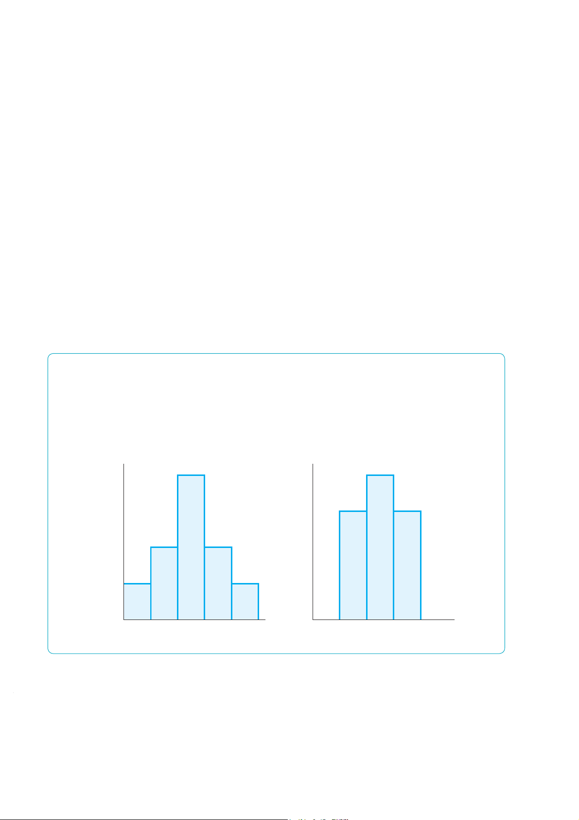
dry city. The probability that it rains no days during the month is 10%, as is the
probability of exactly four days of rain. The chance of two rainy days is 40%, and
the chance of one or three rainy days is 20% each. The probability that it rains five or more days a month is 0%.
Figure 17.1 Probability Distributions
The probability distribution shows the probability of
month is 0%. The probability distributions in panels a and
occurrence for each of the mutually exclusive outcomes.
b have the same mean. The variance is smaller in panel b,
Panel a shows five possible mutually exclusive outcomes.
where the probability distribution is more concentrated
The probability that it rains exactly two days per month
around the mean than the distribution in panel a.
is 40%. The probability that it rains five or more days per (a) Less Certain (b) More Certain 40 40 Probability Probability distribution distribution Probability, % 30 Probability, % 30 20 20 10 10 10% 20% 40% 20% 10% 30% 40% 30% 01234 01234 Days of rain per month Days of rain per month 17.1 Assessing Risk 565
These weather outcomes are mutually exclusive—only one of these outcomes can
occur at a given time—and exhaustive—no other outcomes than those listed are pos-
sible. Where outcomes are mutually exclusive and exhaustive, exactly one of these
outcomes will occur with certainty, and the probabilities must add up to 100%. For
simplicity, we concentrate on situations with only two possible outcomes. Expected Value
One of the common denominators I have found is that expectations rise above that
which is expected. —George W. Bush
Gregg, a promoter, schedules an outdoor concert for tomorrow. How much money 2
he’ll make depends on the weather. If it doesn’t rain, his profit or value from the
concert is V=15. (If it will make you happier—and it will certainly make Gregg
happier—you can think of the profits in this example as $15,000 instead of $15.) If
it rains, he’ll have to cancel the concert and he’ll lose V=-5, which he must pay
the band. Although Gregg does not know what the weather will be with certainty,
he knows that the weather department forecasts a 50% chance of rain.
Gregg may use the mean or the average of the values from both outcomes as a
summary statistic of the likely payoff from booking this concert. The mean or aver- age value is called his (here, his expected value
expected profit). The expected value,
EV, is the value of each possible outcome times the probability of that outcome:3
EV=[Pr(no rain) *Value(no rain)] +[Pr(rain) *Value(rain)] =[ 12*15] +[ 1 2*(-5)] =5,
where Pr is the probability of an outcome, so Pr(rain) is the “probability that rain occurs.”
The expected value is the amount Gregg would earn on average if the event were
repeated many times. If he puts on such concerts many times over the years and the
weather follows historical patterns, he will earn 15 at half of the concerts without
rain, and he will get soaked for -5 at the other half of the concerts, at which it rains.
Thus, he’ll earn an average of 5 per concert over a long period of time. Solved Problem
Suppose that Gregg could obtain perfect information so that he can accurately predict 17.1
whether it will rain far enough before the concert that he could book the band only
if needed. How much would he expect to earn, knowing that he will eventually have
this perfect information? How much does he gain by having this perfect information? Answer
1. Determine how much Gregg would earn if he had perfect information in each
state of nature. If Gregg knew with certainty that it would rain at the time of
the concert, he would not book the band, so he would make no loss or profit:
V=0. If Gregg knew that it would not rain, he would hold the concert and make 15.
2My brother Gregg, a successful concert promoter, wants me to inform you that the hero of the
following story is some other Gregg who is a concert promoter.
3With n possible outcomes, the value of outcome i is Vi, and the probability of that outcome is Pri,
the expected value is EV=Pr1V1+Pr2V2+c+PrnVn. 566 CHAPTER 17 Uncertainty
2. Determine how much Gregg would expect to earn before he learns with certainty
what the weather will be. Gregg knows that he’ll make 15 with a 50% probability
(= 12) and 0 with a 50% probability, so his expected value, given that he’ll receive
perfect information in time to act on it, is EV=( 1 2*15) +( 1 2*0) =7.5.
3. Calculate his gain from perfect information as the difference between his expected
earnings with perfect information and his expected earnings with imperfect infor-
mation. Gregg’s gain from perfect information is the difference between the
expected earnings with perfect information, 7.5, and the expected earnings with-
out perfect information, 5. Thus, Gregg expects to earn 2.5 (=7.5 -5) more
with perfect information than with imperfect information.4
Comment: Having information has no value if it doesn’t alter behavior. This infor-
mation is valuable to Gregg because he avoids hiring the band if he knows that it will rain.
Variance and Standard Deviation
From the expected value, Gregg knows how much he is likely to earn on average if
he books many similar concerts. However, he cannot tell from the expected value how risky the concert is.
If Gregg’s earnings are the same whether it rains or not, he faces no risk and the
actual return he receives is the expected value. If the possible outcomes differ from one another, he faces risk.
We can measure the risk Gregg faces in various ways. The most common approach
is to use a measure based on how much the values of the possible outcomes differ
from the expected value, EV. If it does not rain, the difference between Gregg’s actual
earnings, 15, and his expected earnings, 5, is 10. The difference if it does rain is
-5-5=-10. It is convenient to combine the two differences—one difference for
each state of nature (possible outcome)—into a single measure of risk.
One such measure of risk is the variance, which measures the spread of the prob-
ability distribution. For example, the variance in panel a of Figure 17.1, where the
probability distribution ranges from zero to four days of rain per month, is greater
than the variance in panel b, where the probability distribution ranges from one to three days of rain per month.
Formally, the variance is the probability-weighted average of the squares of the
differences between the observed outcome and the expected value.5 The variance of
the value Gregg obtains from the outdoor concert is
Variance =[Pr(no rain) *(Value(no rain) -EV) ] 2
+[Pr(rain) *(Value(rain) -EV) ] 2 =[ 12*(15 -5)2]+[ 12*(- - 5 5)2] =[ 12*(10)2]+[ 1 2*(-10)2]=100.
4This answer can be reached directly. The value of this information is his expected savings from not
hiring the band when it rains: 1 2*5=2.5.
5With n possible outcomes, an expected value of EV, a value of Vi for each outcome i, and Pri
probability of each outcome i, the variance is
Pr1(V1-EV)2+Pr2(V2-EV)2+g+Prn(Vn-EV)2.
The variance puts more weight on large deviations from the expected value than on smaller ones. 17.2 Attitudes Toward Risk 567
Table 17.1 Variance and Standard Deviation: Measures of Risk Outcome Probability Value Deviation
Deviation2Deviation2:Probability No rain 1215 10 100 50 Rain 1 -5 -10 100 50 2 Variance 100 Standard Deviation 10
Note:Deviation =Value -EV=Value -5.
Table 17.1 shows how to calculate the variance of the profit from this concert step
by step. The first column lists the two outcomes: rain and no rain. The next column
gives the probability. The third column shows the value or profit of each outcome.
The next column calculates the difference between the values in the third column and
the expected value, EV=$5. The fifth column squares these differences, and the last
column multiplies these squared differences by the probabilities in the second column.
The sum of these probability weighted differences, $100, is the variance.
Instead of describing risk using the variance, economists and businesspeople often
report the standard deviation, which is the square root of the variance. The usual
symbol for the standard deviation is
σ (sigma), so the symbol for variance is σ2.
For the outdoor concert, the variance is σ2=$100 and the standard deviation is σ=$10. 17.2 Attitudes Toward Risk
Given the risks Gregg faces if he schedules a concert, will Gregg stage the concert?
To answer this question, we need to know Gregg’s attitude toward risk. Expected Utility
If Gregg did not care about risk, then he would decide whether to promote the con-
cert based on its expected value (profit) regardless of any difference in the risk.
However, most people care about risk as well as expected value. Indeed, most people
are risk averse—they dislike risk. They will choose a riskier option over a less risky
option only if the expected value of the riskier option is sufficiently higher than that of the less risky one.
We need a formal means to judge the trade-off between expected value and risk—
to determine if the expected value of a riskier option is sufficiently higher to justify
the greater risk. The most commonly used method is to extend the model of utility
maximization. In Chapter 4, we noted that one can describe an individual’s prefer-
ences over various bundles of goods by using a utility function. John von Neumann
and Oskar Morgenstern (1944) extended the standard utility-maximizing model to
include risk.6 This approach can be used to show how people’s taste for risk affects
6This approach to handling choice under uncertainty is the most commonly used method.
Schoemaker (1982) discusses the logic underlying this approach, the evidence for it, and several
variants. Machina (1989) discusses a number of alternative methods. Here we treat utility as a
cardinal measure rather than an ordinal measure.