Bài báo cáo môn Hệ thống truyền động Servo đề tài "Matlab Simulation and PID Algorithm Servo Control"

lOMoARcPSD| 37054152
Ministry of Education and Training
HCMC University of Technology and Educatiton
Faculty of HighQuality Training Mechatronics Department COURSE REPORT
Subject: Drive Servo System
MATLAB SIMULATION AND PID ALGORITHM OF SERVO CONTROL Index
1. Simulation of 3 levels of velcoity for NL= 5 and NL=7 ................................................... 6
1.1 Situation 1: NL = 5........................................................................................................... 6
1.1.1 Low velocity which is equivalent to 1st order ............................................................ 6
1.1.2 Middle velocity which is equivalent to 2nd order ..................................................... 10
1.1.3 High speed which is equivalent to 4th order .............................................................. 12 1.2 Situation 1: NL =
7.......................................................................................................191.2.1 Low velocity
which is equivalent to 1st order ........................................................................................... 15
1.2.2 Middle velocity which is equivalent to 2nd order ..................................................... 18
1.2.3 High speed which is equivalent to 4th order..............................................................27
1.3 Position and velocity response comment for 3 velocity levels:..................................30
2. PID Algorithm.................................................................................................................31 lOMoAR cPSD| 37054152 Requirements:
Q1: Each group has to choose the load parameters including soft-coupling stiffness (KL), inertia moment (J
) to satisfy the condition: 3 ≤ L), and viscous damping (DL
𝑁𝑁 ≤ 10 and 0 ≤ 𝑁
≤ 0.02 (at least 2 different loads in this range)
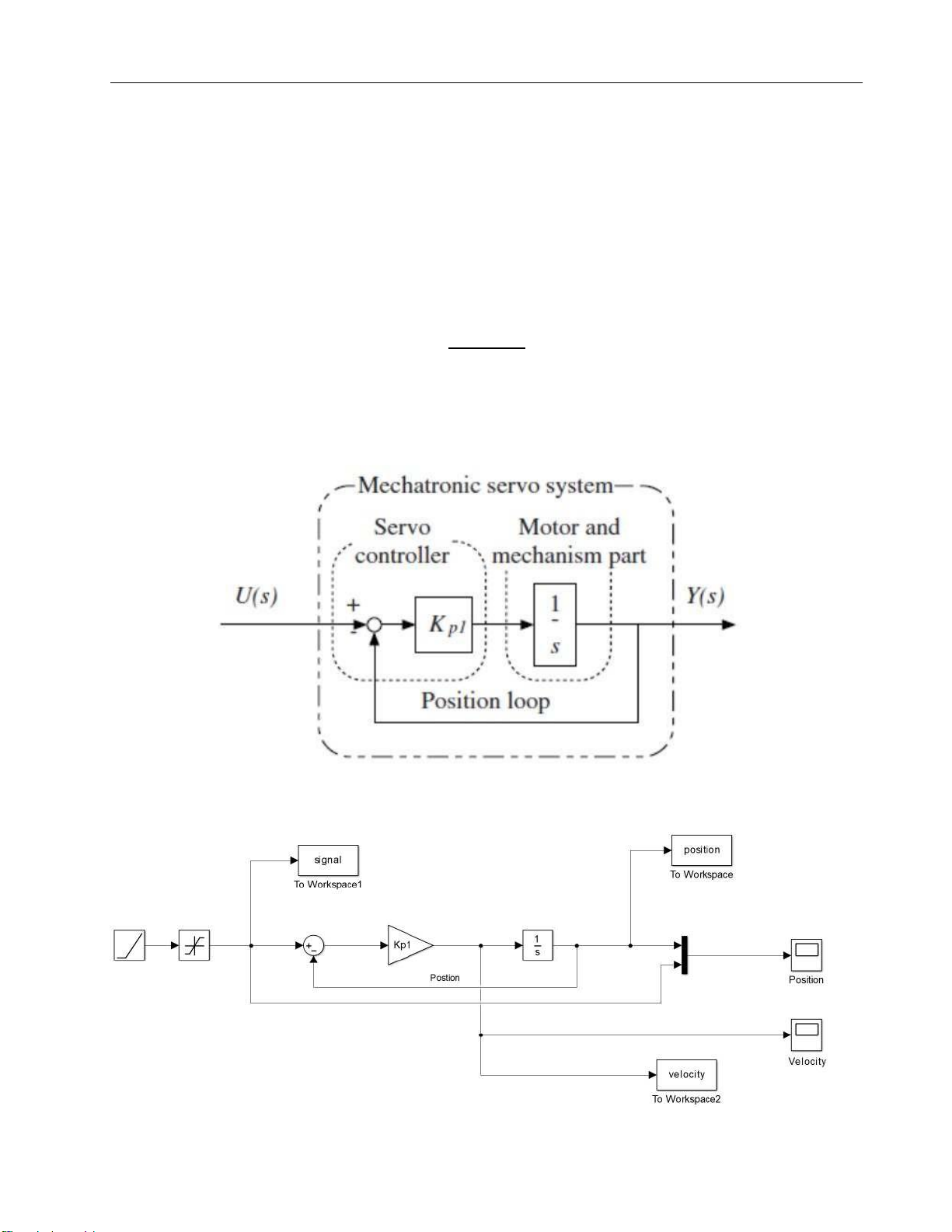
1. Create a simulink block diagram for a single axis servo system
2. Calculate all necessary parameters including load parameters and controlparameters
3. Simulate position responses at 3 different speed levels: - High speed - Middle speed - Low speed
Q2: Each group uses the motor in question 1. Write the PID algorithm using m-file of Matlab
to simulate to velocity control of the motor. The algorithm has to include the derivative filter
for D-term and anti-windup for I-term. Illustrate the effect of anti-windup in your results? 1 lOMoARcPSD| 37054152 Drive Servo System
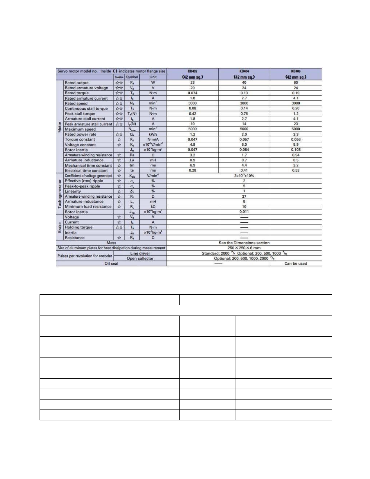
Figure 1. Datasheet of the motor KB404 Motor
Sanyo Denki – KB404 – 24VDC
Motor Characteristics Rated output (PR) W 40
Rated armature voltage (VR) V 24 Rated torque (TR) N.m 0.13
Rated armature current (IR) A 2.7 Rated speed (NR) min-1 3000
Continous stall torque (TS) N.m 0.14
Peak stall torque (TP(N)) N.m 0.76
Armature stall current (IS) A 2.7
Peak armature stall current (IP(N)) A 14 Maximum speed (Nmax) min-1 5000 lOMoAR cPSD| 37054152 Drive Servo System Rated power rate (QR) kW/s 2 Torque constrant (KT) N.m/A 0.057 Voltage constrant (KE) x10-3V/min-1 6.0 Rotor Inertia (JM) x10-4kg.m2 0.084
Armature winding resistance (Ra) Ω 1.7
Armature inductance (La) mH 0.7
Mechanical time constrant(tm) ms 4.4
Electrical time constrant(te) ms 0.41
Tachogenerator Option
Cofficient of votage generated (KEG) V/min-1 3x10-3 ± 10%
Effective (rms) ripple(ɛs) % 2
Peak-to-peak ripple (ɛs) % 5 Linearity(δL) % 1
Armature winding resistance(R1) Ω 37
Armature inductance(L1) mH 5
Minimum load resistance (RL) kΩ 10 Rotor inertia (JTG) x10-4kg.m2 0.011 Brake Voltage (VB) V Current (IB) A Holding torque (TB) N.m Inertia (JB) x10-4kg.m2 Resistance (RB) Ω
Encoder Specifications Items Unit Specifications Encoder type Incremental encoder Pulses per revolution P/R
Standard 2000 (Optional: 200, 500, 1000) Output circuit Line driver lOMoAR cPSD| 37054152 Drive Servo System Output phase difference
T2 to 6 = 1/4T0 ± 1/8T0 Zero-point signal T6 = T0 ± 0.4T0 Operating temperature oC 0 to +85 (inside the encoder) Inertia X10-4kgm2 0.005 Number of channels 3 Power supply VDC +5±5% Current consumption mA 160 max VDC VOH = 2.4 min., VOL = 0.5max. Output circuit voltage at I0 = ± 20 mA Output circuit current mA 20 max. Response frequency kHz 200 PWM duty cycle T1 = 1/2T0 ± 1/8T0 3
Table 1.1 Datasheet of the KB404 motor Rated ouput of motor kW 0.2 Rated torque of motor kgm 0.195 Rated velocity of motor rev/min 1000
Inertia moment of motor axis Jm kgm2 0.00224
Inertia moment of mechanism JL kgm2 0.00653
Natural angle frequency of mechanism part ωL rad/s 94.2
Damping rate of mechanism part xL 0.002 Encoder resoluion pulse/rev 2000
Gear deceleration ratio NG 1 lOMoAR cPSD| 37054152 Drive Servo System
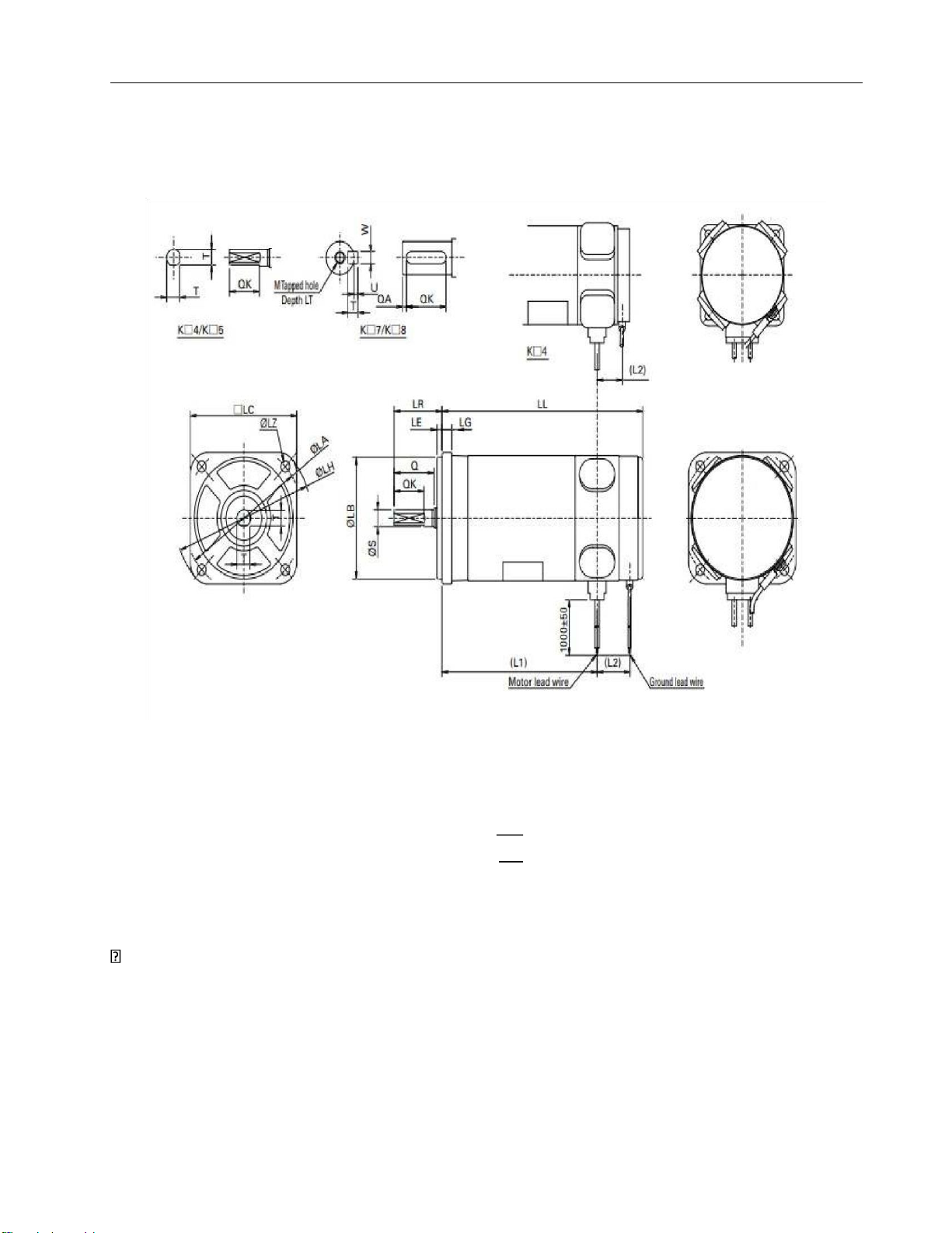
Figure 2. Sanyo Deiki KB404 Motor Drawing
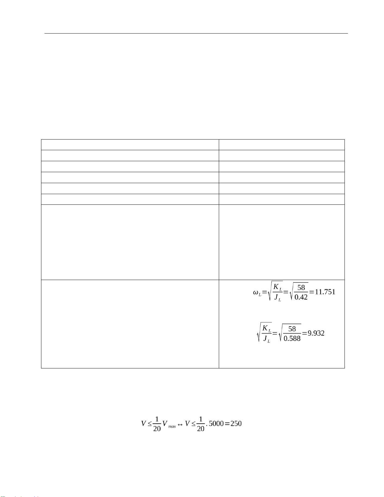
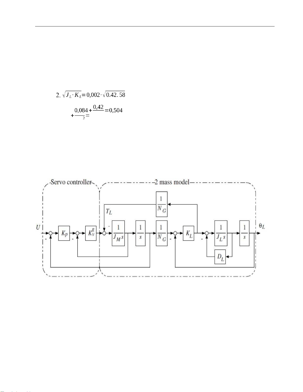
Table 1.2 Lecture Slide
From the Table 1.2, we choose the hardness of solf joint KL √ ωL= JL K 2
L=ωL .JL=(94,2)2.0,00653=57,95 (N .m) lOMoARcPSD| 37054152 Drive Servo System
Thus, we choose the joint hardness KL=58(N .m)
The motor may have a gear box but in the simulation, we choose NG = 1
Q1 requires selecting at least 2 loads in the range from 3 to 10. Hence, we choosing NL = 5 and NL = 7
1. Simulation of 3 levels of velcoity for NL= 5 and NL=7 Power, P (W) 40 Max speed Nmax (rpm) 5000
Inertia JM (x 10-4kg.m2) 0.084
Damping rate if mechanism part xL 0.002
Spring constrant of mechanism part KL (N.m) 58
Gear deceleration ratio NG 1
Inertia moment of mechanism part JL (x 10-4 + With NL =5 kgm2) J 2 L = NL.NG .JM = 5.1.0,084 = = 0.42 + With NL=7 J 2 L = NL.NG .JM = 7.1.0,084= = 0.588
Natural angle frequence of mechanism part ωL (rad/s) + With N L = 5 + With NL = 7 ωL=
*Note: In order to show clearly all reponses for whole velocity levels, our group decided to
select 200 rad for position to simulate the graph.
1.1 Situation 1: NL = 5
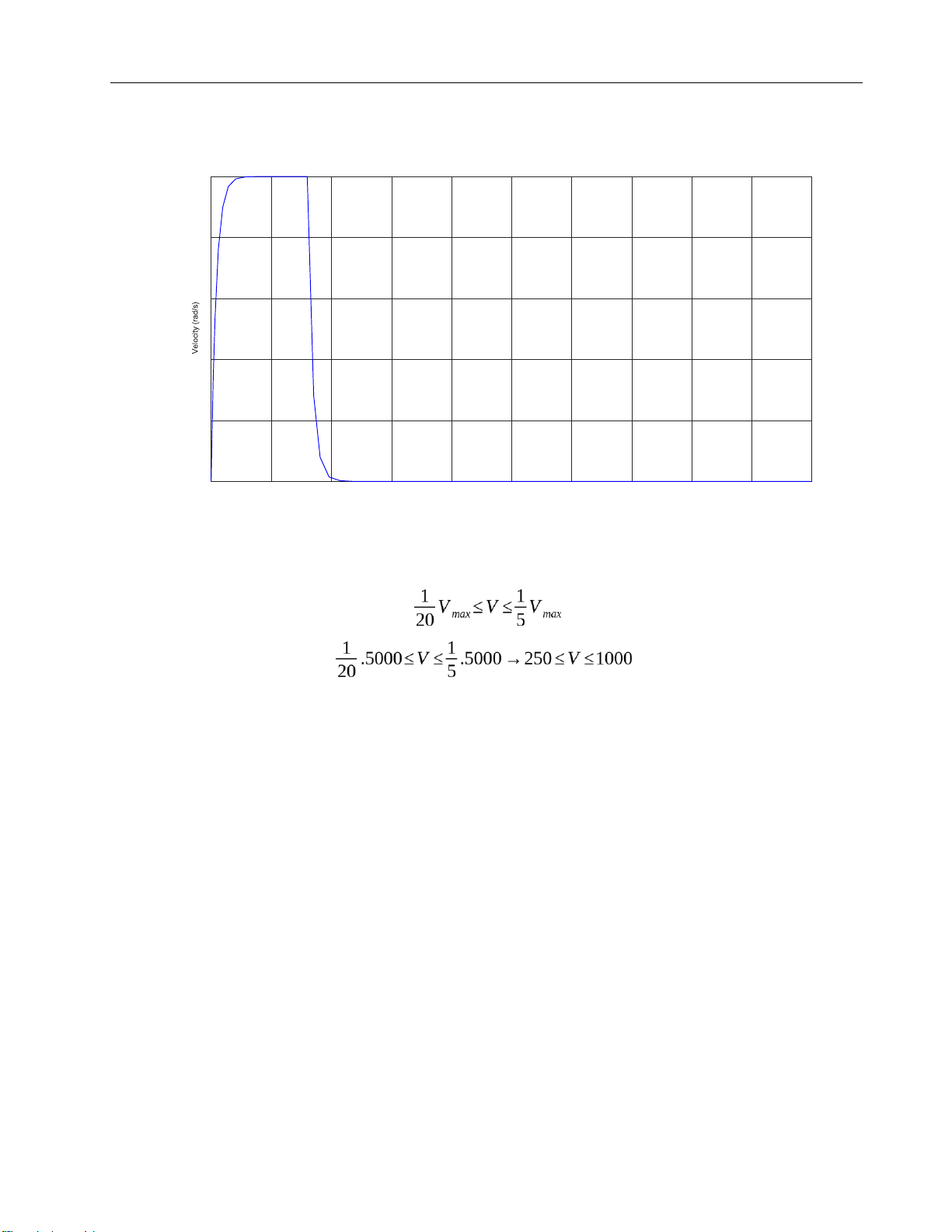
1.1.1 Low velocity which is equivalent to 1st order rpm
V ≤26,2rad/s = lOMoARcPSD| 37054152 Drive Servo System Choose V = 25 rad/s cp = 0,24; cv = 0,82
b0 = (1+NL) cpcv = (1+5).0,24.0,82=1,1808
b1 = (1+NL) (cv+2cpcvxL) = (1+5) (0,82 + 2.0,24.0,82.0,002) = 4,925 b0 1,1808
cp1=b1= 4,925 =0,24
Kp1=cp1.ωL=0,24.11.751=2.82024
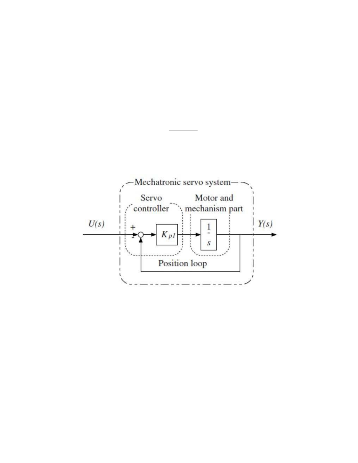
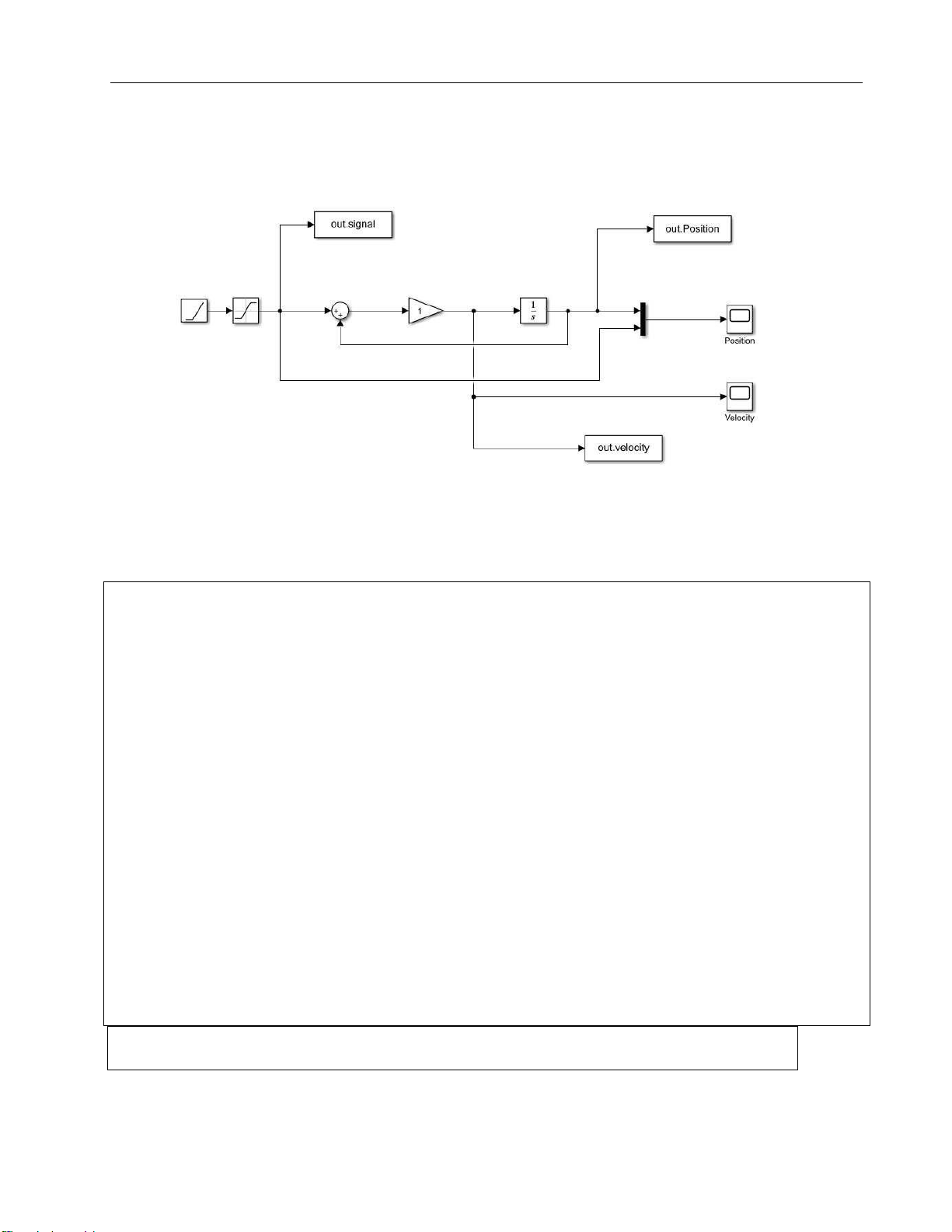
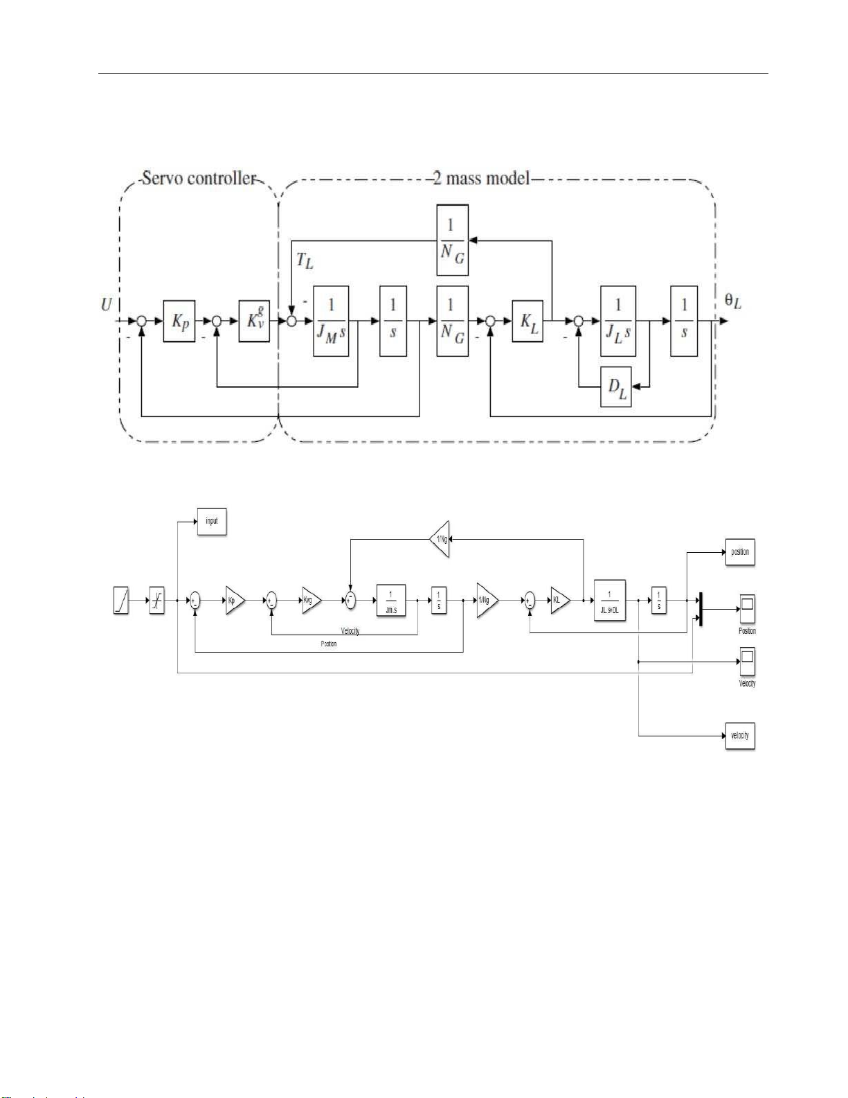
Figure 3. 1st order model of a servo system = lOMoARcPSD| 37054152 Drive Servo System
Figure 4. 1st order model modified in Matlab Simulink Code for simulation: clc clear all NL = 5; Ng = 1; Cp = 0.24; cv = 0.82; psi = 0.02; Jm = 0.084; KL = 58; % Formular JL = NL*Jm*(Ng^2); wL = sqrt(KL/JL); DL = 2*psi*sqrt(KL*JL); b0=(1+NL)*cp*cv; b1=(1+NL)*(cv+2*cp*cv*psi); cp1=b0/b1; Kp1 = cp1*wL; sim('Bac1_nl5') % matlab drawing hold on
plot(signal.Time, signal.Data, '--k', 'LineWidth',1) plot(position.Time, position.Data, '-r', 'LineWidth',1) legend('Input','Position')
%plot(velocity.Time, velocity.Data, '-r', 'LineWidth',1) grid on = lOMoARcPSD| 37054152 Drive Servo System
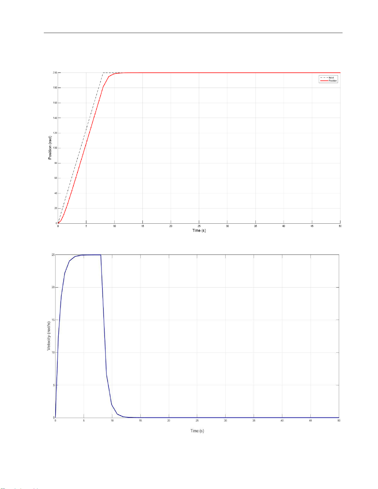
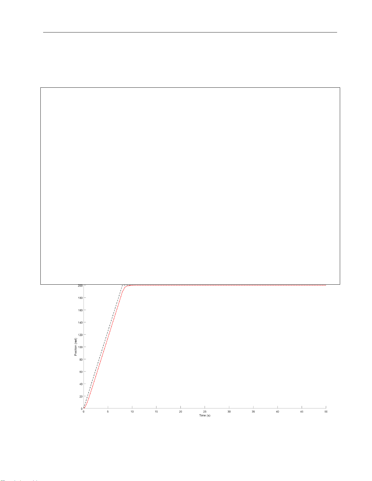
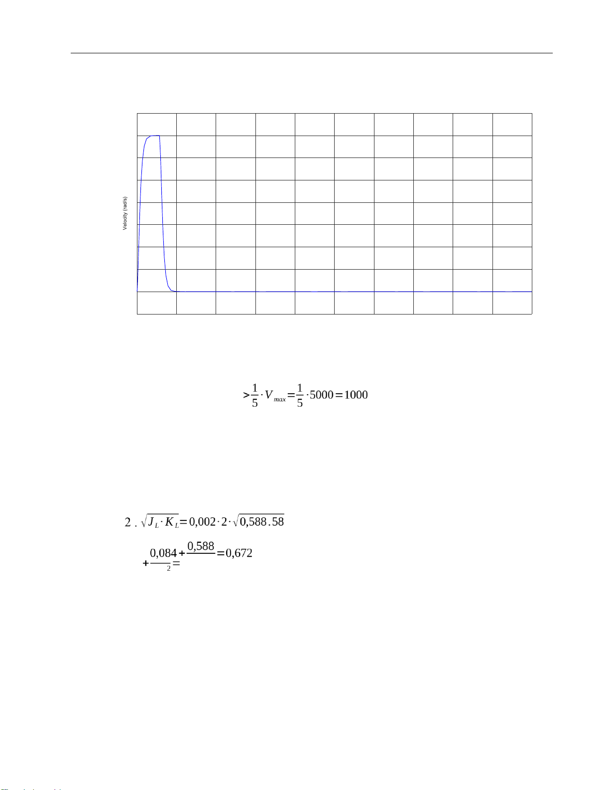
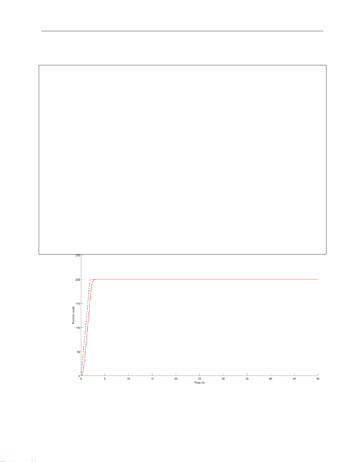
Figure 5. Graph of position in 1st order at position = 200 rad
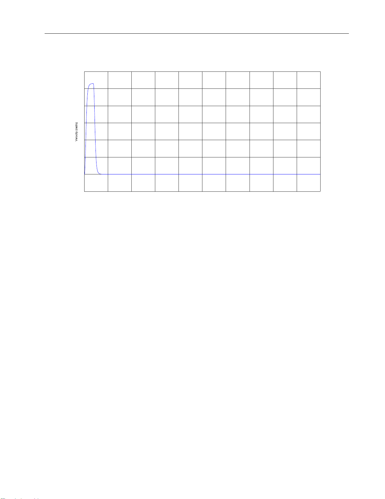
Figure 6. Graph of velocity in 1st order = lOMoARcPSD| 37054152 Drive Servo System
1.1.2 Middle velocity which is equivalent to 2nd order → rpm
→26,2≤V≤104,7rad/s Choose V = 100 rad/s
We have cp2 = 0,24; cv2 = 0,96
Kp2 = ωL.cp2= 0,24. 11,751 = 2,82024
Kv2 =ωL.cv2=¿0,96. 11,751 = 11,281
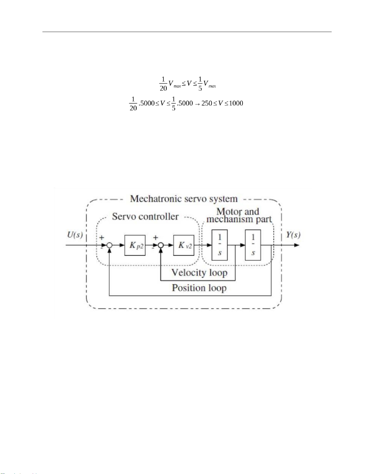
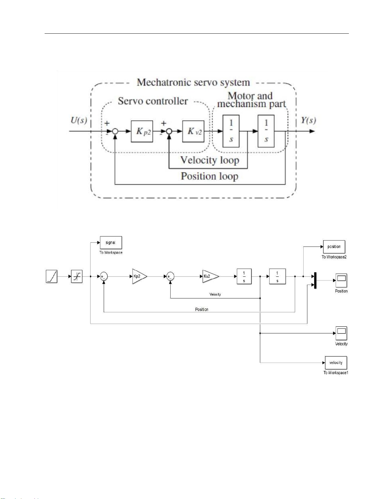
Figure 7. 2nd order model of a servo system = lOMoARcPSD| 37054152 Drive Servo System
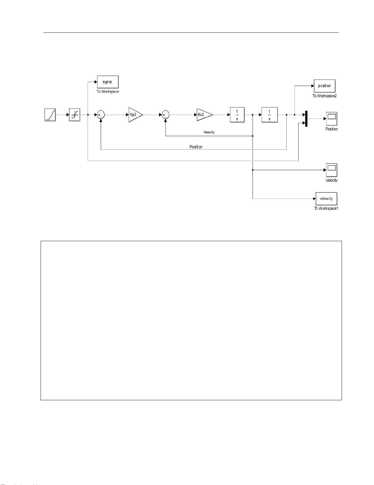
Figure 8. 2nd order model modified in Matlab Simulink Code for simulation: clc clear all cp2=0.24; cv2=0.96; KL=58; NL=5; Jm=0.084; Ng=1; JL = NL*Jm*(Ng^2); wL = sqrt(KL/JL); Kp2=cp2*wL; Kv2=cv2*wL; sim('Bac2_NL5') %ve do thi matlab hold on
plot(signal.Time, signal.Data, '--k', 'LineWidth',1) plot(position.Time, position.Data, '-r', 'LineWidth',1) legend('Input','Postion')
%plot(velocity.Time, velocity.Data, '-b', 'LineWidth',1) grid on = lOMoARcPSD| 37054152 Drive Servo System Time (s)
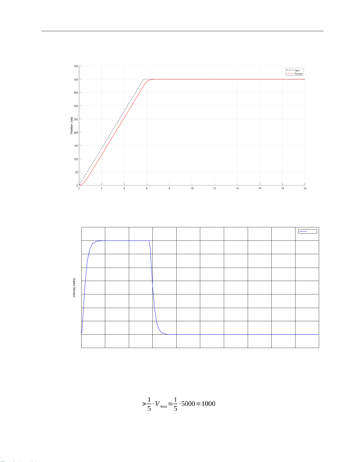
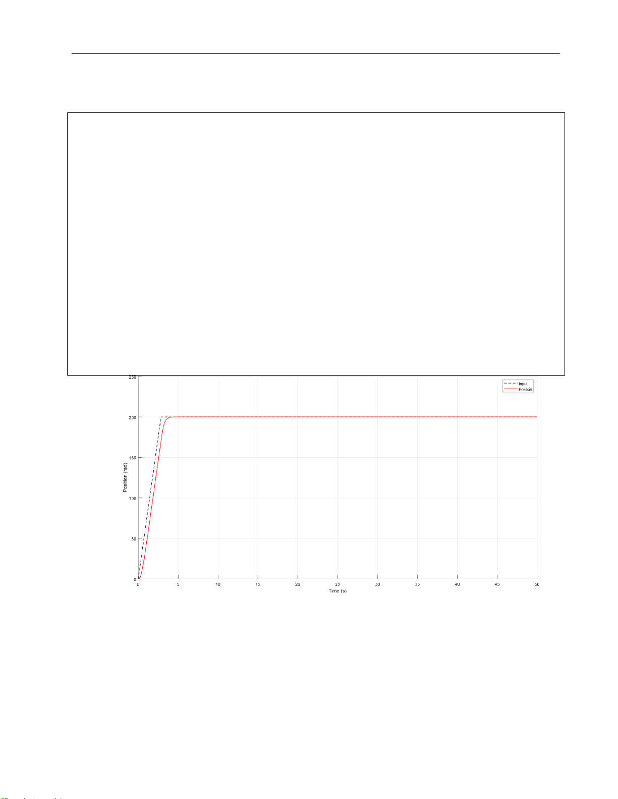
Figure 9. Graph of position in 2nd order at position = 400 rad 80 Velocity 70 60 50 40 30 20 10 0 -10 0 2 4 6 8 10 12 14 16 18 20 Time (s)
Figure 10. Graph of velocity in 2nd order
1.1.3 High speed which is equivalent to 4th order V rpm
→V>104,7rad/s = lOMoARcPSD| 37054152 Drive Servo System Choose V = 106 rad/s cp = 0,24; cv = 0,82 J 2
L = NL.NG .JM = 5.1. 0,084 = 0,42 DL = xL. = 0,0098 JL JT = JM NG 1
Kp = cp ∙ωL = 0,24. 11,751 = 2,82024
Kv = cv ∙ωL = 0,82. 11,751 = 9,63582
Kvg = Kv. JT = 9,63582. 0,504 = 4,856
Figure 11. 4th order model of a servo system = lOMoARcPSD| 37054152 Drive Servo System
Figure 12. 4th order model modified in Matlab Simulink Code for simulation: clc clear all cp=0.24; cv=0.82; KL=58; Ng=1; Jm=0.084; psi=0.002; NL=5; %cong thuc cho bac 4 JL = NL*Jm*(Ng^2); wL = sqrt(KL/JL); DL=psi*2*sqrt(JL*KL); JT=Jm+(JL/(Ng^2)); Kp=cp*wL; Kv=cv*wL; Kvg=Kv*JT; sim('Bac4_NL5') %ve do thi matlab hold on
plot(input.Time, input.Data, '--k', 'LineWidth',2) plot(position.Time, position.Data, '-r', 'LineWidth',2) legend('Input','Position')
plot(velocity.Time, velocity.Data, '-b', 'LineWidth',2) grid on = lOMoARcPSD| 37054152 Drive Servo System
Figure 13. Graph of position in 4th order at position = 200 rad
Figure 14. Graph of velocity in 4th order
1.2 Situation 1: NL = 7
1.2.1 Low velocity which is equivalent to 1st order rpm
V ≤26,2rad/s = lOMoARcPSD| 37054152 Drive Servo System Choose V = 25 rad/s cp = 0,24 ; cv = 0,82
b0 = (1+NL)cpcv = (1+7).0,24.0,82=1,5744
b1 = (1+NL)(cv+2cpcvxL) = (1+7)(0,82 + 2.0,24.0,82.0,002) = 6,566 b0 1,5744
cp1=b1= 6,566 =0,24
Kp1=cp1.ωL=0,24.9,932=2,38368
Figure 15. 1st order model of a servo system = lOMoARcPSD| 37054152 Drive Servo System
Figure 16. 1st order model modified in Matlab Simulink Code for simulation: clc clear all NL=7; Ng=1; cp=0.24; cv=0.82; psi=0.02; Jm=0.084; KL=58; % Calculate the coefficents JL = NL*Jm*(Ng^2); wL = sqrt(KL/JL); DL = 2*psi*sqrt(KL*JL); b0=(1+NL)*cp*cv; b1=(1+NL)*(cv+2*cp*cv*psi); cp1=b0/b1; Kp1 = cp1*wL; sim('Bac1_NL5') % Plot hold on
plot(signal.Time, signal.Data, '--k', 'LineWidth',1) plot(position.Time, position.Data,
'-r', 'LineWidth',1) legend('Input','Position')
%plot(velocity.Time, velocity.Data, '-r', 'LineWidth',1) grid on
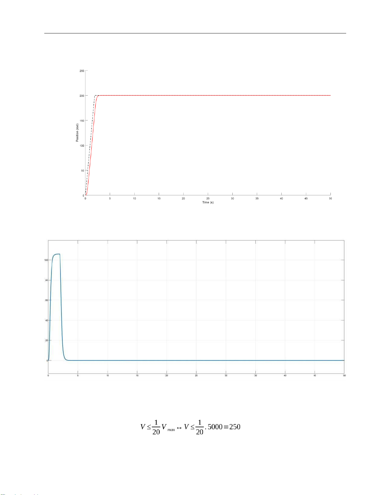
Figure 17. Graph of position in 1st order at position = 200 rad = lOMoARcPSD| 37054152 Drive Servo System 25 20 15 10 5 0 0 5 10 15 20 25 30 35 40 45 50 Time (s)
Figure 18. Graph of velocity in 1st order
1.2.2 Middle velocity which is equivalent to 2nd order → rpm
→26,2≤V≤104,7rad/s Choose V = 100 rad/s
We have cp2 = 0,24 ; cv2 = 0,96
Kp2 = ωL.cp2= 0,24 . 9,932 = 2,38368
Kv2 =ωL.cv2=¿0,96 . 9,932 = 9,53472 = lOMoARcPSD| 37054152 Drive Servo System
Figure 19. 2nd order model of a servo system
Figure 20. 2nd order model modified in Matlab Simulink Code for simulation: = lOMoARcPSD| 37054152 Drive Servo System clc clear all cp2=0.24; cv2=0.96; KL=58; NL=7; Jm=0.084; Ng=1; JL = NL*Jm*(Ng^2); wL = sqrt(KL/JL); Kp2=cp2*wL; Kv2=cv2*wL; sim('Bac2_NL5') % Plot hold on
plot(signal.Time, signal.Data, '--k', 'LineWidth',1) plot(position.Time, position.Data, '-
r', 'LineWidth',1) legend('Input','Postion')
% plot(velocity.Time, velocity.Data, '-b', 'LineWidth',1) grid on
Figure 21. Graph of position in 2nd order at position = 200 rad = lOMoARcPSD| 37054152 Drive Servo System 80 70 60 50 40 30 20 10 0 -10 0 5 10 15 20 25 30 35 40 45 50 Time (s)
Figure 22. Graph of velocity in 2nd order
1.2.3 High speed which is equivalent to 4th order V rpm
→V>104,7rad/s Choose V = 106 rad/s cp = 0,24 ; cv = 0,82 J 2
L = NL . NG . JM = 7 . 1 . 0,084 = 0,588 DL = xL . = 0,023 JL JT = JM NG 1
Kp = cp ∙ωL = 0,24 . 9,932 = 2,38368
Kv = cv ∙ωL = 0,82 . 9,932 = 8,14424
Kvg = Kv . JT = 8,14424 . 0,672 = 5,473 = lOMoARcPSD| 37054152 Drive Servo System
Figure 23. 4th order model of a servo system
Figure 24. 4th order model modified in Matlab Simulink Code for simulation: = lOMoARcPSD| 37054152 Drive Servo System clc clear all cp=0.24; cv=0.82; KL=58; Ng=1; Jm=0.084; psi=0.002; NL=7;
% Formula for the 4 order JL =
NL*Jm*(Ng^2); wL = sqrt(KL/JL); DL=psi*2*sqrt(JL*KL); JT=Jm+(JL/(Ng^2)); Kp=cp*wL; Kv=cv*wL; Kvg=Kv*JT; sim('Bac4_NL5') % Plot hold on
plot(input.Time, input.Data, '--k', 'LineWidth',1) plot(position.Time, position.Data,
'-r', 'LineWidth',1) legend('Input','Position')
%plot(velocity.Time, velocity.Data, '-b', 'LineWidth',1) grid on
Figure 25. Graph of position in 4th order at position = 200 rad = lOMoARcPSD| 37054152 Drive Servo System 120 100 80 60 40 20 0 -20 0 5 10 15 20 25 30 35 40 45 50 Time (s)
Figure 26. Graph of velocity in 4th order
1.3 Position and velocity response comment for 3 velocity levels: -
The velocity in 3 cases corresponds to each speed level: "Low, medium, high" is 25,
70,106 rad/s respectively. The higher the velocity, the faster the desired position of 200 rad is
achieved. In all 3 cases, we can see there is no overshoot occuring. Hence, it is true to
necessary requirements of the Sevro engine. -
For NL=5 and NL=7 we can see no difference between 3 velocity levels : "Low,
medium, high". Obviously the parameters of the engine can meet in case 3≤NL≤10. Thus, it
satisfies the theoretical basis we have learned = lOMoARcPSD| 37054152 Drive Servo System 2. PID Algorithm
Table 2.1 Necessary parameter for Q2 Motor
Sanyo Denki KB404 – 24V
Vontage constant, Ke (x10-3V/min-1) 6,0
Torque Const., Kt (Nm/A) 0,057
Armature winding resistance, Ra (Ω) 1,7
Armature Inductance, La (mH) 0,7
Rotor Inertia, JM (x 10-4kg.m2) 0,084 Viscous Cofficient (b) 0
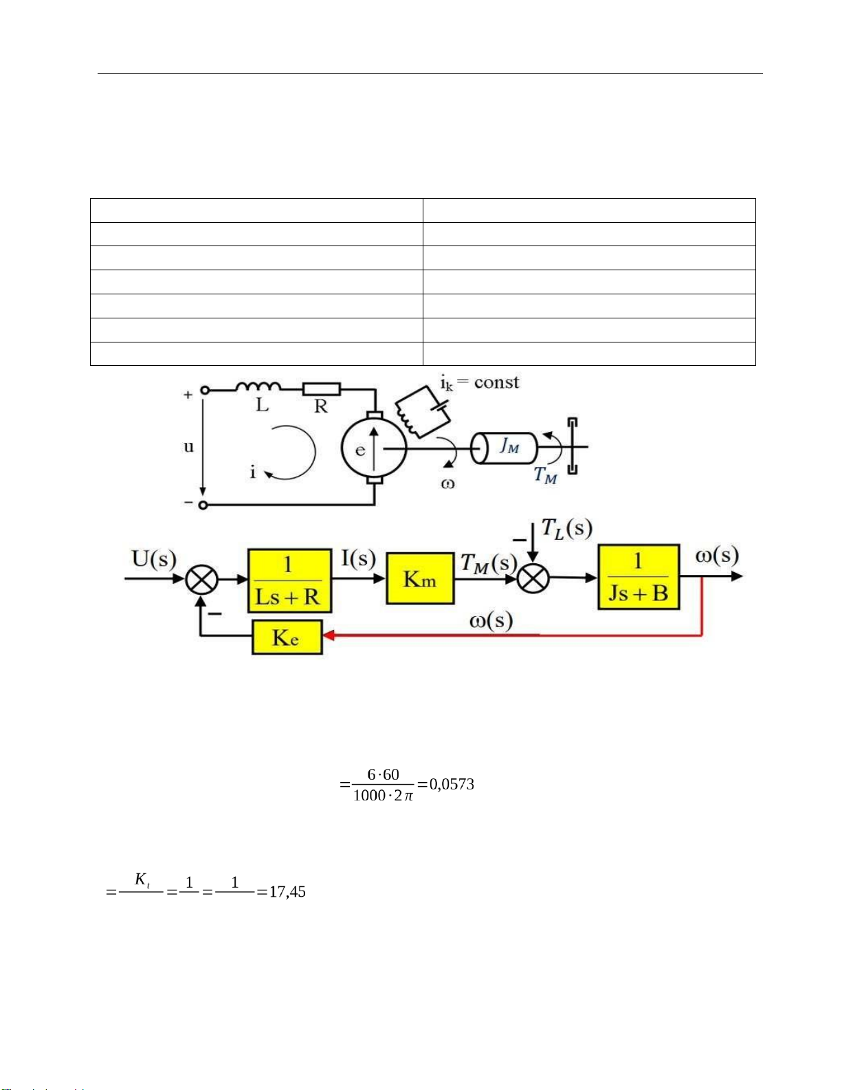
Figure 27. The block diagram of a DC motor
Converting the unit of Ke from 10-3V/min-1 into V/rad/s Ke V /rad/s
Notice that Ke = Kt which is right for the theory learnt
K-factor of DC motor drive function K Kt ∙ Ke K e 0,057 Response time = lOMoARcPSD| 37054152 Drive Servo System Ra∙J M
1,7∙0,084∙10−4 τ= = =0,0044(s)
Kt ∙K e 0,057∙0,057 Desired
response time: τc=0,002(s) Comment:
In the simulation of the PID algorithm, the group choose to skip the D stage in sevro DC K
motor control. The motor characteristic has the formula τM s+1 of the first order, so there is no
need to use the D stage. Therefore in the simulation, the group exclusively uses the PI control due to D is 0.
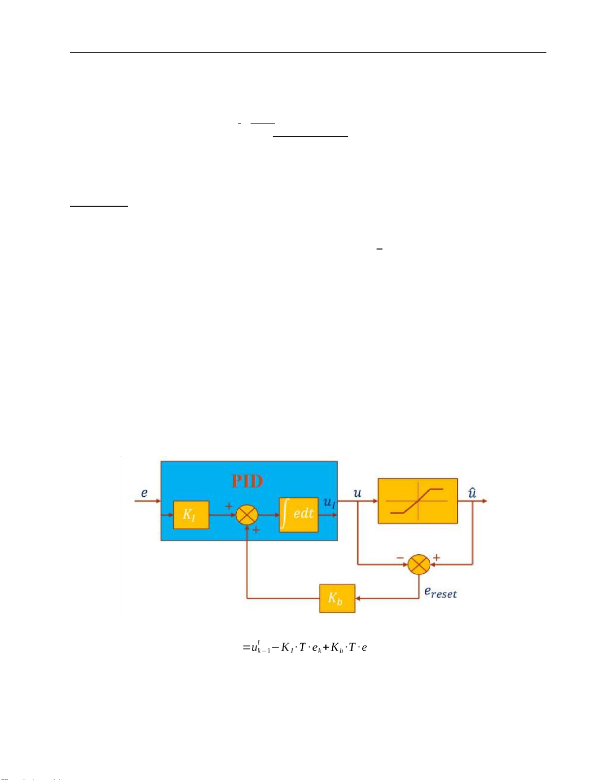
* However in the simulation, our group still program filter for D in order to meet the
requirement P-term calculation: ukp=Kp∙ek Anti-windup:
Figure 28. The anti-windup scheme for I-term uik resetk Low pass filter: = lOMoARcPSD| 37054152 Drive Servo System Figure 29. D- term low pass filter uD N K
f (k )= N +T ∙uDf ( k−1)+
N +DT ∙(e(k)−e(k−1))
PID control’s paramenter including anti-windup for I-term and low pass filter D-term uk Dk
Figure 30. Model in Matlab Simulink = lOMoAR cPSD| 37054152 Drive Servo System Code: PID control: %Parameter Declaration %L, R, Km, Jm, b, Ke
global Ts Kb Kp Ki Kd err_previous e_reset yi_previous yd_f_previous alpha L = 0.3*10^-3; R = 0.44; Km = 0.06; Jm = 0.37*10^-4; b = 0; Ke = 0.06; %Ke = Kt = 0.58 K = 20; tau = 0.0045; % ~0.005 tauc = 0.02; Ts = 0.01; alpha = 0.9;
%Controller Specs: Kp, Kd, Ki, Kb Kp = tau/(K*tauc); Ki = Kp/tau; Kd = 0; Kb = 200; %Anti-windup err_previous = 0; e_reset = 0; yi_previous = 0; yd_f_previous = 0; sim('Simulation2'); %Graph = lOMoARcPSD| 37054152 Drive Servo System
figure(1); plot(yout.Time, yout.Data, '- r','LineWidth', 2) grid on
figure(2); plot(yout1.Time, yout1.Data, '- b','LineWidth', 2) grid on = lOMoARcPSD| 37054152 Drive Servo System PID function: function y = PID_Function(u)
global Ts Kb Kp Ki Kd err_previous e_reset yi_previous yd_f_previous alpha wd = u(1); wf = u(2); err = wd - wf; %Calculating P-term yp = Kp * err; %Low pass filter D-term yd = Kd * (err - err_previous)/Ts;
yd_f = (1 - alpha) * yd_f_previous + alpha * yd; %Anti-windup I-term
yi = yi_previous + Ki * err * Ts + Kb * e_reset * Ts; %Output value calculation yk = yp + yi + yd_f; err_previous = err; yi_previous = yi; yd_f_previous = yd_f; %Upper and Lower limits if yk > 24 e_reset = 24 - yk; yk = 24; elseif yk < -24 e_reset = -24 - yk; yk = -24; else e_reset = 0; end y = yk; end = lOMoARcPSD| 37054152 Drive Servo System
In this simulation, we divided into 3 cases: - System with no load.
- Sytem with small load that it’s still responding.
- System with big enough (high) load that its cannot responses.
The load will be applied in 2s, from 2s to 4s: = lOMoARcPSD| 37054152 Drive Servo System
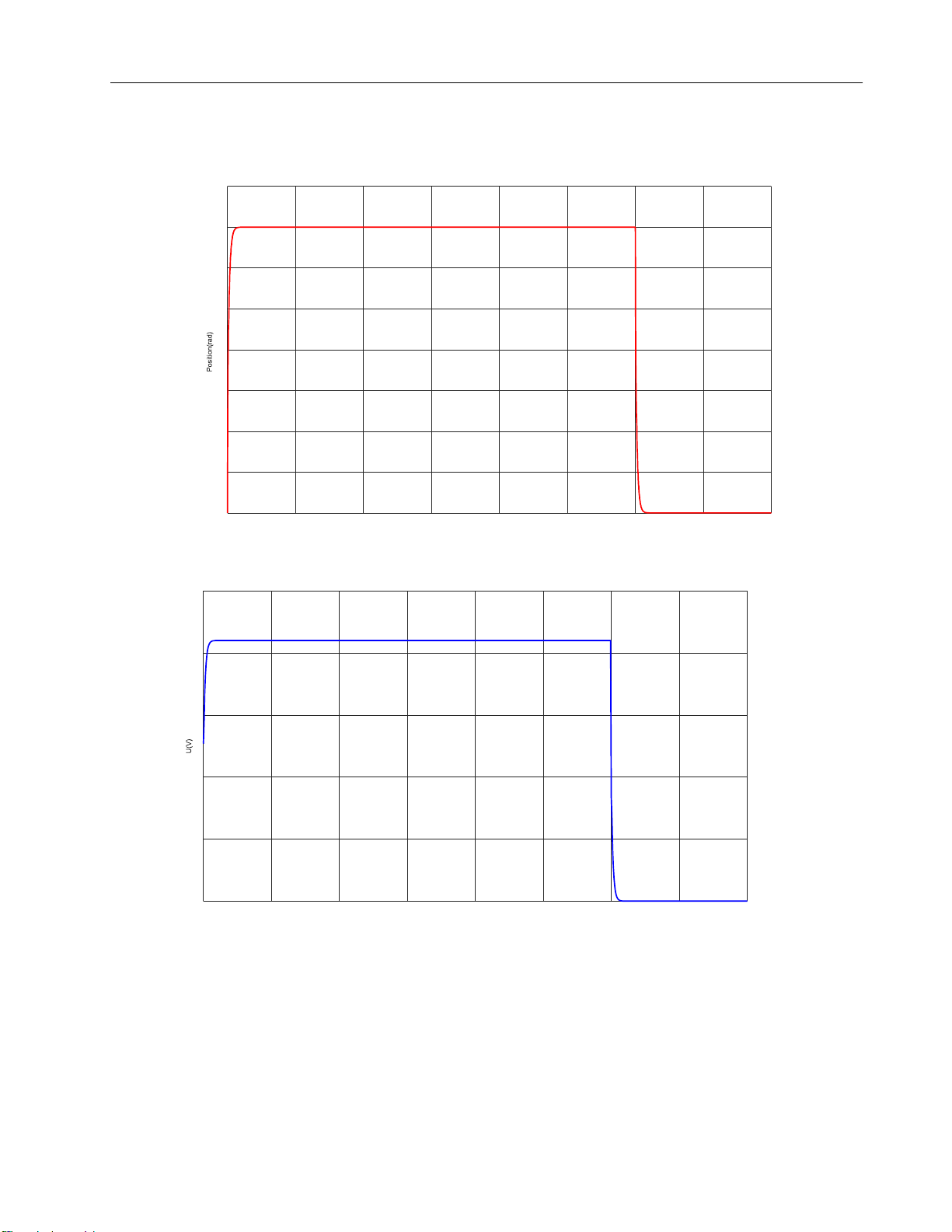
The output speed of position control 400 350 300 250 200 150 100 50 0 0 1 2 3 4 5 6 7 8 Time(s)
Output voltage of PID Controller 25 20 15 10 5 0 0 1 2 3 4 5 6 7 8 Time(s) Figur
e 31: System with no load
The output speed of posotion control = lOMoARcPSD| 37054152 Drive Servo System 400 350 300 250 200 150 100 50 0 0 1 2 3 4 5 6 7 8 Time(s)
Output voltage of PID Controller 25 20 15 10 5 0 0 1 2 3 4 5 6 7 8 Time(s) Figur
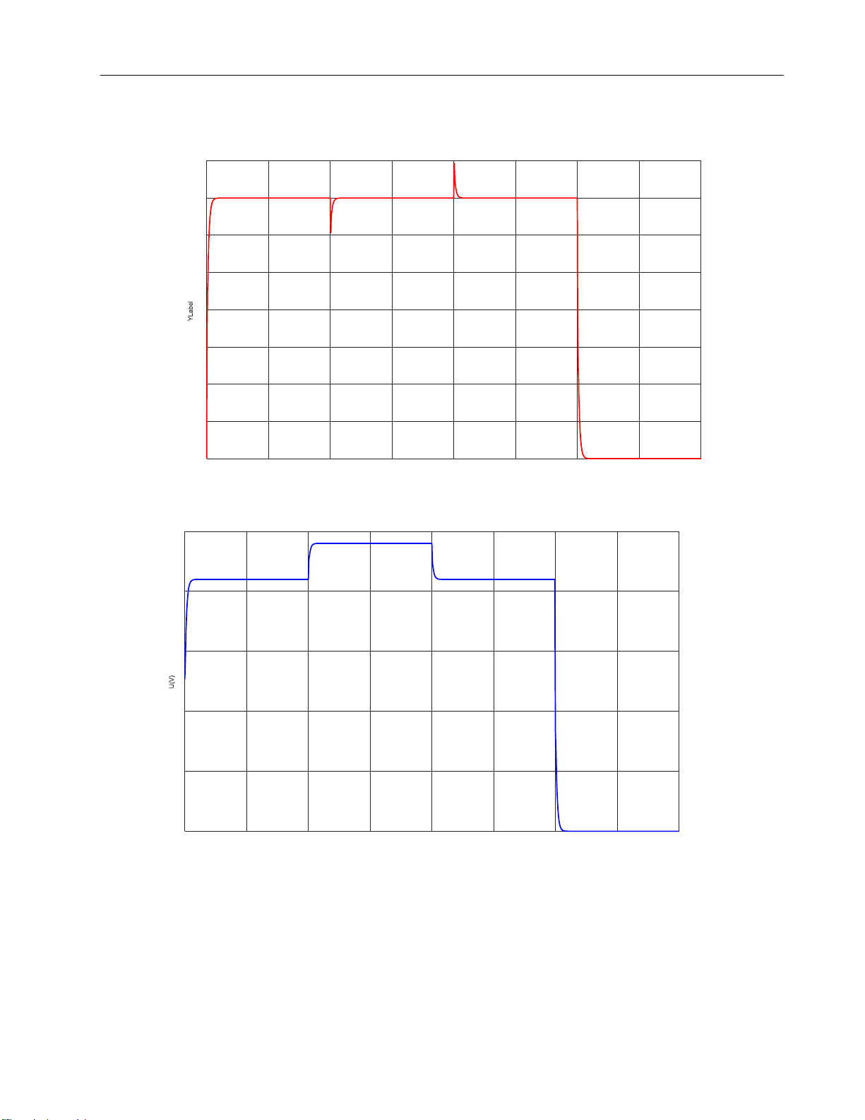
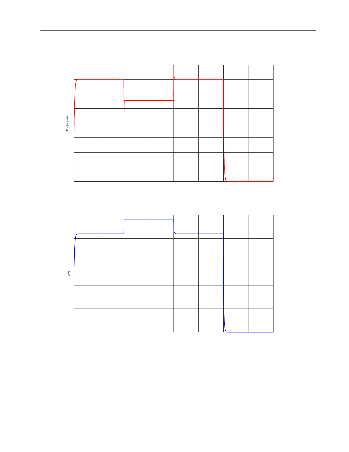
e 32: System with small load Title = lOMoARcPSD| 37054152 Drive Servo System 400 350 300 250 200 150 100 50 0 0 1 2 3 4 5 6 7 8 Time(s)
Output Voltage of PID Controller 25 20 15 10 5 0 0 1 2 3 4 5 6 7 8 Time(s)
Figure 33: System with high load Comment: Figure 32:
When the magnitude of the noise is small, the graph noise is still deflected down, but
in a short period of time, the graph can still return to its original position. The magnitude of = lOMoAR cPSD| 37054152 Drive Servo System
the noise is less or not much greater than the moment of the engine, it will immediately return to its original position. Figure 33:
Because the load parameter is too large than the moment of the engine, when there is
an impact load for a period of 2 to 4 seconds, the engine cannot return to its original position like Figure 32 =