Bài báo cáo môn Hệ thống truyền động Servo: Matlab Simulation | Đại học Sư phạm Kỹ thuật Thành phố Hồ Chí Minh

BỘ GIÁO DỤC VÀ ĐÀO TẠO
TRƯỜNG ĐẠI HỌC SƯ PHẠM KĨ THUẬT TP.HCM
KHOA ĐÀO TẠO QUỐC TẾ SERVO REPORT MATLAB SIMULATION
COURSE: SERV334029E_23_1_01FIE
Instructor: M.S Võ Lâm Chương GROUP 4
Ho Chi Minh City, December 2023 lOMoARcPSD| 37054152 I. Question 1:
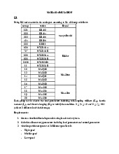
Using DC servo motors in the catalogues according to No. of Group as follows:
Each group has to choose the load parameters including soft-coupling stiffness (KL),
inertia moment (JL), and viscous damping (DL) to satisfy the condition: 3 ≤ ≤ 10 and 0
≤ ≤ 0.02 (at least 2 different loads in this range)
Group 4 ,so we practice on Sanyo Denki Brand ( KB506 series) lOMoARcPSD| 37054152
1. Create a simulink block diagram for a single axis servo system
- Highspeed 4th ordermodel:
- Middle speed2nd ordermodel: lOMoARcPSD| 37054152
- Lowspeed1st order model: lOMoARcPSD| 37054152
2. Calculate all necessary parameters including load parameters and control parameters
From the KB506 catalogue, we have some fixed parameters:
Rotor inertia:JM=0.22×10−4 (kg.m2)Rated speed:N R=3000 (min−1)
We choose Gear Ratio:NG=1
In an industrial servo system, the following conditions are used successfully: - 3≤N L≤10 - 0≤ξL≤0.02
Shaft’s diameter = 7 (mm)
Torque = 1 (N.m), Angular = 1o
Torque 1 K L= Angular = π =57.296¿ 1× o 180
We suppose the first load have: N L=4 lOMoARcPSD| 37054152 ξ L=0.01
Calculate J L: JL 2 2 −4 −4 2 N L=
2 =¿J L=N L×NG ×J M=4×1 ×0.22×10 =0.88×10 (kg.m ) NG J M
Calculate DL: D L 2√ J L KL L L
Calculate ωL: (rad /s)
Servo controller for 4th cp=0.24,cv=0.82
K p=c pωL=0.24×806.9=193.656
Kv=cv ωL=0.82×806.9=661.658 JL −4 0.88×10−4 −4 2 JT=J M+ N2 =0.22×10 + 1
=1.1×10 (kg.m ) G K g
v =Kv J T=661.658×1.1×10−4=0.07278238 lOMoARcPSD| 37054152
Position response of single axis servo system 12 Position 10 8 6 4 2 0 0 0.05 0.1 0.15 0.2 0.25 0.3 0.35 0.4 0.45 0.5 Time (s) 600
Velocity response of single axis servo system Velocity 500 400 300 200 100 0 -100 0 0.05 0.1 0.15 0.2 0.25 0.3 0.35 0.4 0.45 0.5 Time (s)
Servo controller for 2nd: lOMoARcPSD| 37054152
vo => 250rpm ≤v2≤ 1000rpm => We choose: v2=60 rad/s
cp2=0.234303566,cv2=4cp2=0.9372114264
K p2=cp2ωL=0.234303566×806.9=189.059
Kv2=cv2ωL=0.9372114264×806.9=756.237
Position response of single axis servo system 12 Position 10 8 6 4 2 0 0 0.05 0.1 0.15 0.2 0.25 0.3 0.35 0.4 0.45 0.5 Time (s) lOMoARcPSD| 37054152
Velocity response of single axis servo system 70 Velocity 60 50 40 30 20 10 0 -10 0 0.05 0.1 0.15 0.2 0.25 0.3 0.35 0.4 0.45 0.5 Time (s)
Servo controller for 1st: v0= 5000rpm = 523 (rad/s) v v = 250rpm =
π(rad/s)
We choose: v1=26rad/s Calculate ωL: √ K L 806.899 ωL= JL =
b0=(1+N L)c p cv=(1+4 )∗0.24∗0.82=0.984 b1=(1+NL)(cv+2cpc vξL)+2N Lξ L
= (1+4)(0.82+2*0.24*0.82*0.01) + 2*4*0.01 =4.19968 b0 lOMoARcPSD| 37054152 cp1=c p2= =0.234303566 b1
=>K p1=cp1ωL=189.059
Position response of single axis servo system 11 10 Position 9 8 7 6 5 4 3 2 1 0 0 0.5 1 1.5 2 2.5 3 3.5 4 4.5 5 TIME (S)
Velocity response of single axis servo system 30 Velcocity 25 20 15 10 5 0 0 0.5 1 1.5 2 2.5 3 3.5 4 4.5 5 Time(s) lOMoARcPSD| 37054152
We suppose the second load have: N L=10 ξ L=0.02
Calculate J L: JL 2 2 −4 −5 2 N L=
2 =¿JL=N L×NG ×JM=10×1 ×0.047×10 =4.7×10 (kg.m ) NG J M
Calculate DL: D L 2√ J L KL L L L L
Servo controller for 4th cp=0.24,cv=0.82
K p=c pωL=0.24×1104.11=264.99
Kv=cv ωL=0.82×1104.11=905.37 JL −4 4.7×10−5 −5 2 JT=J M+ N2 =0.047×10 + 1 =5.17×10 (kg.m ) G K g
v =Kv J T=905.37×5.17×10−5=0.047