Bài báo Nghiên cứu khoa học nói về nhiệt phân, từ science direct

Applied Mathematical Modelling 33 (2009) 3756–3767
Contents lists available at ScienceDirect Applied Mathematical Modelling
j o u r n a l h o m e p a g e : w w w . e l s e v i e r . c o m / l o c a t e / a p m
Aerodynamics of an isolated slot-burner from a tangentially-fired boiler
J.T. Hart a, J.A. Naser a,*, P.J. Witt b
a Faculty of Engineering and Industrial Science, Swinburne University of Technology, John Street, Hawthorn, VIC 3122, Australia
b CSIRO Division of Minerals, Clayton 3168, Australia a r t i c l e i n f o a b s t r a c t Article history:
The aerodynamic development of fully turbulent isothermal jets issuing from rectangular Received 9 July 2007
slot-burners was modelled by obtaining a solution to the Reynolds averaged Navier–Stokes
Received in revised form 14 November 2008
equations. A finite-volume method was used with the standard k–e, RNG k–e and Reynolds Accepted 22 December 2008
stress turbulence models. The slot-burners were based on physical models, which were
Available online 8 January 2009
designed to be representative of typical burner geometries found in tangentially-fired coal
boilers. Two cases were investigated, in which jets from three vertically stacked rectangu-
lar nozzles discharged at 90° and then 60° to the wall containing the burner. The nozzle Keywords:
angle had little effect on jet centreline velocity decay, with the 60° nozzle showing a mar- Slot-burner Tangentially-fired boiler
ginally higher rate of decay. The jets from the 60° nozzles were found to deviate slightly Rectangular jet
from their geometric axis slightly due to internal pressure redistribution in the flow at RANS model
the nozzles. The simulations were validated against the physical models and were found
to reproduce the flow field of the jets accurately with the Reynolds stress model producing the best results.
Ó 2009 Elsevier Inc. All rights reserved. 1. Introduction
Stable combustion in a tangentially-fired boiler is achieved by orienting the burner jets so as to induce a swirling vortex in
the central region of the boiler, providing enhanced mixing and extending the residence time of the fuel to ensure complete
burnout (see Fig. 1). A burner set may contain several burners located in a vertical plane, with a single burner consisting of a
primary fuel/air nozzle, sandwiched between secondary air nozzles above and below. There is significant separation between the nozzles.
In gas fired and black-coal fired boilers the flames are anchored to the nozzle and most of the combustion occurs in the
near-field of the jet. In the near-field of burner jets in a lignite-fired boiler the lignite particles undergo pyrolysis and volatile
matter is driven from the particle, but only a limited amount of combustion occurs, therefore turbulent mixing in the near-
field of the jets is less crucial. The main aims are to heat the coal and air by mixing it with entrained hot furnace gases and
deliver it to the correct location in the centre of the furnace. Near-field aerodynamics is still important for entrainment and
for ensuring that the jets reach the centre of the furnace at the correct location and with sufficient momentum to generate the required swirl.
The level of combustion in the near-field is low enough that aerodynamics are sufficiently decoupled from the effects of
intense chemical reaction and radiative heat transfer, which would otherwise alter the physical properties of the flow. There-
fore, isothermal modelling can reasonably be expected to give a good indication how the jets from different burner geom-
etries deliver the fuel stream and mix it with the surrounding hot combustion gases within the furnace.
* Corresponding author. Tel.: +61 392148655.
E-mail address: jnaser@swin.edu.au (J.A. Naser).
0307-904X/$ - see front matter Ó 2009 Elsevier Inc. All rights reserved. doi:10.1016/j.apm.2008.12.020
J.T. Hart et al. / Applied Mathematical Modelling 33 (2009) 3756–3767 3757
Fig. 1. Schematic of boiler indicating firing circle of burner jets.
The objective of this study was a burner geometry used in the Yallourn power station in the Latrobe Valley of Victoria,
Australia. Previous investigations by the boiler operator [1,2], in which scaled-down physical models were made of relevant
burner geometries, provided measurements of velocity made with a Pitot tube and Reynolds stress measurements made
with a hot-wire anemometer. Isothermal aerodynamic modelling was performed on several isolated burner geometries.
Three-dimensional effects are very important in such complex flows, and if modelled correctly, the full flow field prediction
from a computational fluid dynamics (CFD) model can provide more insight into the burner aerodynamics than physical
modelling. The aim of this research was to produce an accurate and well-validated numerical model of the isothermal burner
geometry and use the results to better understand the near-field aerodynamic development of the jets within the burner.
This understanding will be valuable to future burner designs.
2. Numerical models and procedures used
The CFD code CFX4 was used to model the fluid flow, which was subsonic, isothermal, single phase and fully turbulent.
The resulting simplified Reynolds averaged Navier–Stokes (RANS) system of equations solved in this numerical model was
for a constant density, constant temperature, and steady state flow: r ðUÞ ¼ 0; ð1Þ r ðqU UÞ ¼ r ðr qu uÞ; ð2Þ where r is the stress tensor r ¼ pd þ lðrU þ ðrUÞTÞ: ð3Þ
Here q is the fluid density, U = (U, V, W) is the mean velocity vector, p is the pressure, l is the molecular viscosity and qu u is the Reynolds stress term.
Closure of (2) by calculation of qu u was achieved using the k–e model [3], the RNG k–e model [4], and the Reynolds
stress model (RSM) [5]. Wall functions were applied based on the approach of Ref. [6].
Discretisation of the governing equations into a set of algebraic equations was achieved by a control-volume approach on
a body-fitted grid. Two discretisation schemes were employed, a hybrid linear upwind/central differencing and a modified
QUICK scheme known as CCCT [7], which is bounded to prevent non-physical overshoots in k and e.
The SIMPLER (SIMPLE-Revised) method [8] was used as the solution algorithm, and the Rhie and Chow method [9] was
employed to prevent chequerboard oscillations in the pressure.
3. Model geometry and boundary conditions
The burners were based on the physical models of Ref. [1], who designated their models Geometry A, B, C and D. Only
Geometries A and B were modelled in the current study, which are illustrated in Fig. 2. Geometry A comprised a nearly
square primary jet flanked above and below by rectangular secondary jets and discharged orthogonal from a wall into a large
room. Geometry B was the same as Geometry A but the jets made an angle of 60° to the wall. Slot-burners very similar to
Geometry B are found in the Yallourn Stage I boilers. The physical model was approximately 1/30th geometric scale of a real
burner nozzle, with the Reynolds number maintained at around 1 105. Geometrically similar jets exhibit similar behaviour
when the Reynolds number is above 2.5 104 [10] therefore the model burner jets should exhibit aerodynamic behaviour
similar to a full size burner jet. A comparison between the aerodynamic properties of jets in the physical model and the real furnace is shown in Table 1. 3758
J.T. Hart et al. / Applied Mathematical Modelling 33 (2009) 3756–3767
Fig. 2. Burner configurations. Table 1
Comparison of Yallourn and physical/CFD model nozzles. Property Yallourn nozzle Model nozzle Primary jet
Reynolds number (based on hydraulic diameter) 4.6 105 1.3 105 Slot width 1020 mm 37.5 mm Height 800 mm 29.0 mm Gas velocity 39.2 m s1 60 m s1 Secondary jet
Reynolds number (based on hydraulic diameter) 3.8 105 9.3 104 Slot width 1020 mm 37.5 mm Height 565 mm 17.0 mm Gas velocity 32.5 m s1 60 m s1 Base between jets Base height 1020 mm 37.5 mm Width 380 mm 14.0 mm
For each jet the physical model used a section of ducting, which extended 52 hydraulic diameters upstream from the noz-
zle and was fed from a plenum chamber, to achieve a developed flow at the nozzle. The CFD model assumed that the jets
discharged into an infinitely large space. The open atmosphere was approximated by making the domain large enough to
ensure that the steep gradients in the jet shear layer were contained well within the model domain and then placing Dirich-
let constant pressure boundary conditions at the open boundaries. A symmetry boundary condition was placed at the pri-
mary jet centre plane. Dirichlet boundary conditions were set on the inlet for all jets by specifying a flat 60 m s1 velocity
profile at the inlets. Turbulence quantities at the inlet were set based on 1% turbulence intensity, which is appropriate for
a flow coming from a plenum chamber. 4. Grids and grid dependence
The solution domain was constructed using a body-fitted coordinate system and a hexahedral mesh, which mapped the
geometrical features of the domain. A uniform, high-density mesh was used in the duct cross-section and the base region
between the jet nozzles. Outside this region an expansion factor was applied to the grid spacing in the cross-stream direc-
tions where the velocity gradients were shallow. In the stream-wise direction the grid was also coarsened from the nozzle
onwards, although the coarsening was not as rapid, to ensure the entire length of the jet was captured with adequate res-
olution. The jet domain extended approximately one metre in the stream-wise direction, and half a metre in the cross- stream directions.
A grid independence study was performed on Geometry A, as this was the simplest geometry and numerical diffusion was
minimal because the mean flow was predominately aligned with the grid. The tests were performed using the standard k–e
turbulence model with an upwind differencing scheme. Four grid refinements were performed, setting 4 4 cells in the pri-
mary duct cross-section with similar grid distribution everywhere else, then successively doubling the number of cells in the
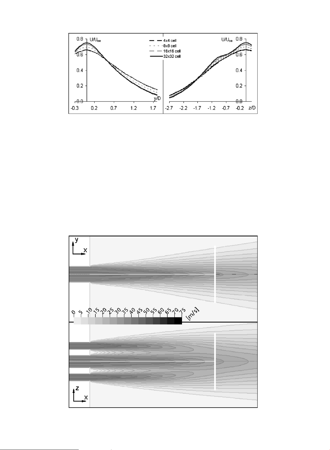
duct cross-sections to 8 8 in the primary then 16 16 and finally 32 32, with appropriate refinement elsewhere. In Fig. 3
the velocity profiles for each grid are compared in the xy plane and xz plane at a distance of 9D downstream of the jet nozzle,
where D is the hydraulic diameter of the primary jet nozzle. This was the farthest point from the nozzle for which
J.T. Hart et al. / Applied Mathematical Modelling 33 (2009) 3756–3767 3759
Fig. 3. Velocity profiles showing grid independence – Geometry A.
experimental data were available, and subsequent comparisons between the simulations and experiment were mainly car-
ried out at this location, making it the most appropriate location to judge the grid dependence. Velocities were normalised to
the centreline exit velocity of the primary jet, UCE.
Change in the profiles was found with each successive grid refinement. The finer grids tended to predict less diffusive jets
with higher centreline velocity and steeper ou/oy and ou/oz profiles. The 32 32 grid gave a very close prediction to that of
the 16 16, especially in the high shear region of y/D P 0.5, and only a three percent difference between the two centreline
velocity predictions. The difference between the 16 16 and 32 32 predictions was small enough to suggest that any fur-
ther grid refinement would yield the same profile in this plane. Based on this, the 32 32 grid was not used, as the extra
computational cost associated with the extra cells did not yielded significantly more accurate results.
Fig. 4. Velocity contours – Geometry A. 3760
J.T. Hart et al. / Applied Mathematical Modelling 33 (2009) 3756–3767 5. Results and discussion
5.1. Geometry A – orthogonal Jets
Fig. 4 shows velocity contours in the xy and xz symmetry planes for the jets in Geometry A as predicted by the standard k–
e model. Velocity comparisons were all made at a plane 9D from the nozzle, the location of which is indicated by thick white
lines. The spreading rate of the primary jet in Geometry A was found by inspection to be 8°. In the xz plane it is shown that
the jets exited the ducts separately, but gradually mixed as their adjacent shear layers interacted, becoming one jet at around
x/D = 10, consistent with the observations of Ref. [11].
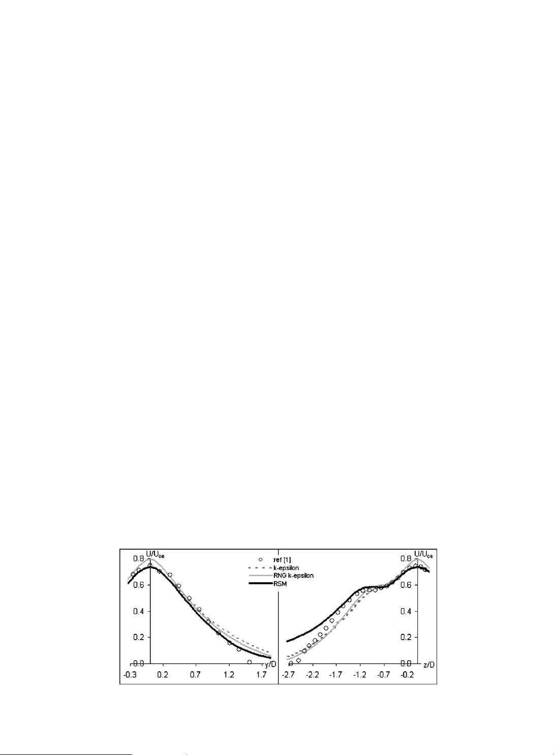
Fig. 5 compares calculated velocity profiles at x/D = 9 in the xy and xz planes using the standard k–e, the RNG k–e and RSM
turbulence models, with the Pitot tube measurements of Ref. [1]. The peak velocity in the core of the jet was well predicted
using the standard k–e and the RSM models, while the RNG k–e model over-predicted it by 7%. In the xy plane both k–e mod-
els showed more spreading than the RSM while the reverse was true in the xz plane. If not for the over-prediction of spread-
ing rate in the outer part of the jet in the xz plane, the RSM model would have given and outstanding comparison with the
physical measurements. Overall, the RSM model did a very good job of matching the magnitude and spatial gradients of the
velocity field, especially in maintaining the presence of a distinct secondary jet profile, which the RNG k–e model also
showed, but the standard k–e model smeared out. The RNG k–e model was somewhat better at predicting the shape and
thickness of shear layers between the jets and the surrounding stagnant fluid than the standard k–e model, however, it some-
what surprisingly over-predicted jet penetration.
Generally, higher values of turbulent kinetic energy, k, were found in the RNG k–e prediction, with the most notable peaks
found on the side edges of the primary jet, and on the top edge of the secondary jet, seen in Fig. 6. Values of e, rate of destruc-
tion of turbulent kinetic energy, were also notably higher in the RNG k–e model. In eddy viscosity turbulence models k and e
are be used to calculate turbulent viscosity and are closely coupled, each one appearing in the other’s transport equation. The
turbulent viscosity predicted by the RNG k–e model was lower than the standard k–e model, the minimum of which was
located in the centre of the primary jet. This lower value accounts for the higher peak velocity in this region, because lower
viscosity means less turbulent shear, and hence less resistance to flow. The turbulent viscosity gradient was also steeper
resulting in the steeper velocity gradient prediction of the RNG k–e model.
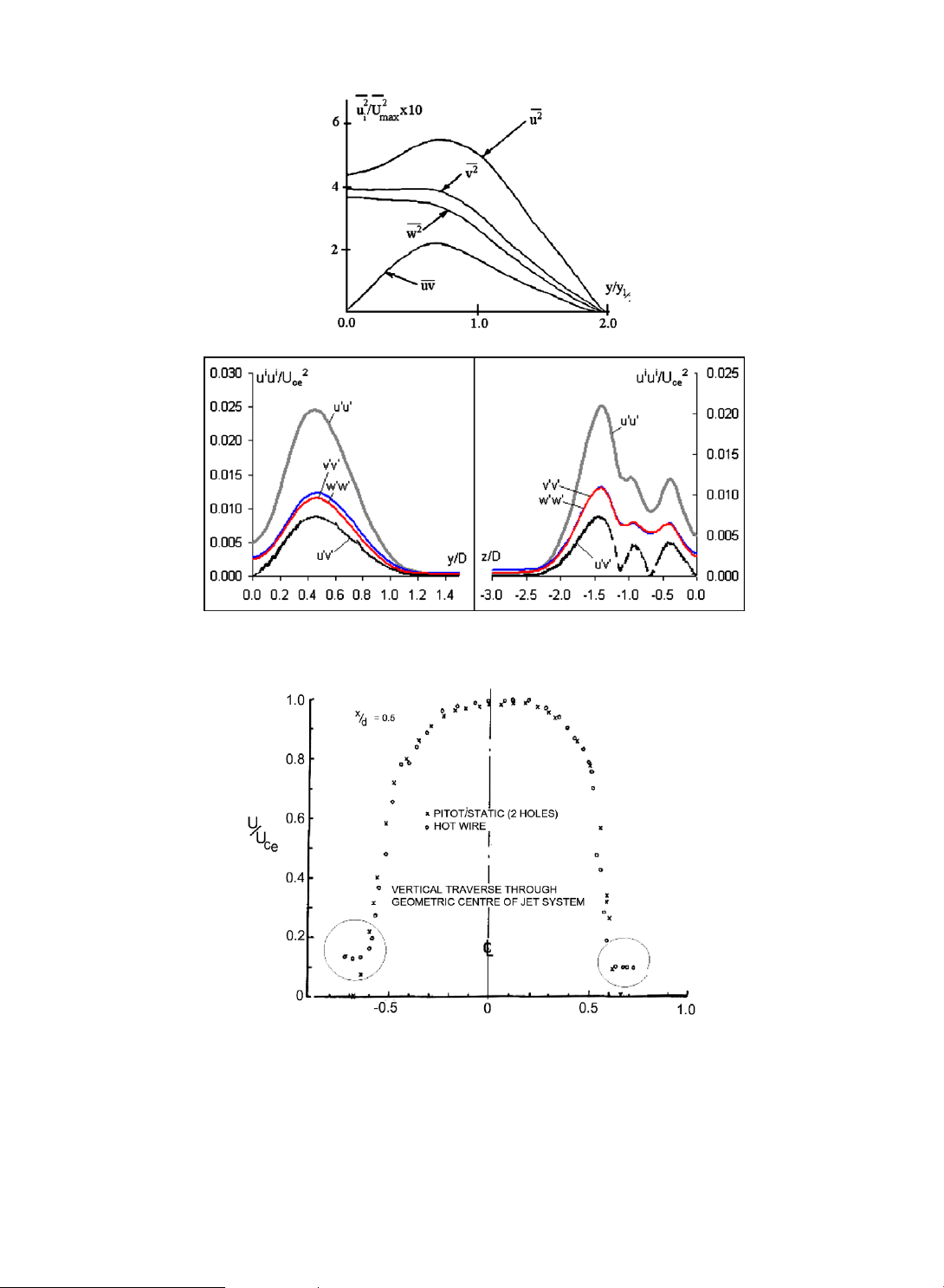
Fig. 7 shows the distribution of turbulent Reynolds stresses calculated by the RSM model at x/D = 5.0, and includes a typ-
ical Reynolds stress distribution for a plane jet [12] for qualitative validation. In a plane jet the normal stresses are all non-
zero at the jet centreline, while the non-zero shear stresses fall to zero on the centreline. Each of the Reynolds stress com-
ponents peaks in the high shear regions, and then tends towards zero away from the jets. The calculated ratio v0/u0 and w0/u0
of 0.75 compared well with literature values of 0.7–0.8 for a single, large aspect ratio, rectangular jet [13–15] and 0.8 for a
square jet [16]. The peak shear stress to peak u0u0 ratio of 0.55 also compared favourably with literature values of 0.3–0.5.
These distributions illustrate the anisotropic nature of the turbulence in these jets, due to the three-dimensional nature
of the flow. The assumption of isotropic turbulence in the derivation of the k–e models has been shown to be false in this
case, which helps to explain why the RSM gave a better prediction overall than the two k–e models.
While the predicted profiles for velocity and turbulent quantities were generally good, none of the profiles exhibited the
same sharp jet boundary that appeared in the measured profiles. Some non-physical diffusion might be expected when using
a turbulence model, however, some doubt exists about the measured experimental data in this region. The measurements
were taken with a pitot tube, which does not measure velocities very well below around 5 m s1. For Geometry B a compar-
ison was made between profiles obtained by Pitot tube and hot-wire anemometry, Fig. 8. For velocities above 15 m s1 (U/
UCE = 0.2) the correlation between Pitot tube and hot-wire was good, but below this the Pitot tube measurements deviated
from those taken by hot-wire. The shear layer of the jet was shown to have a more diffused boundary than the Pitot tube
Fig. 5. Measured and predicted velocity profiles in xy and xz planes – Geometry A.
J.T. Hart et al. / Applied Mathematical Modelling 33 (2009) 3756–3767 3761
Fig. 6. Comparison of k, e and lturb predictions for the two-equation models – Geometry A.
measurements indicated. Had hot-wire data been available for Geometry A, the RSM model predictions of a less sharply de-
fined boundary layer were likely to correlate better with the measured velocity profiles.
5.2. Geometry B – angled Jets 5.2.1. Flow field prediction
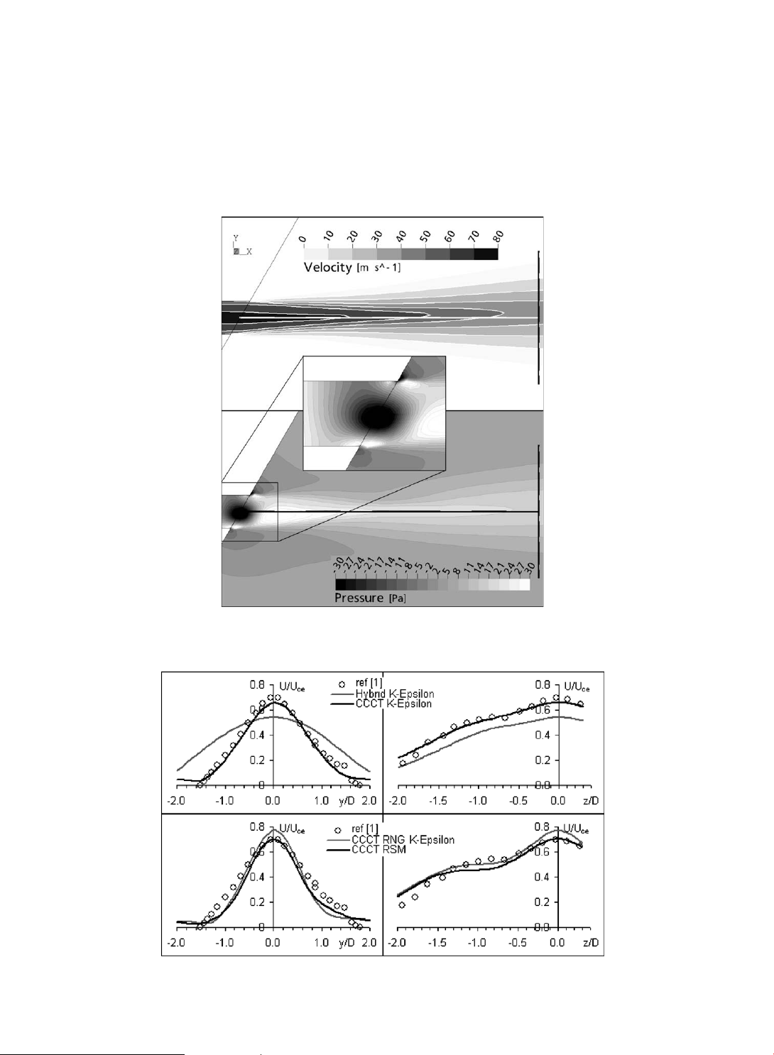
Fig. 9 shows velocity and pressure contours in the xy plane through the middle of the primary jet. The jet centreline devi-
ated away from the geometric axis by 1°, the same amount observed in the physical model [1]. The cause of this deviation
was rooted in several different yet interdependent factors; however, it is difficult to judge the contribution of each factor for
certain with the current results.
The pressure distribution shows a large low-pressure region dominating the centre of the nozzle and a large high-pres-
sure region just downstream of it as a result of the deceleration of the fluid as it entered the open atmosphere. As the jet
exited the duct, it did so earlier on what has been designated the short side. The accompanying pressure rise at the edge
of the nozzle, directly adjacent to the low-pressure region on the middle of the nozzle, resulted in a cross-stream pressure
difference of up to 60 Pa. The main high-pressure region was centred slightly away from the geometric centreline on the
short side. Streamlines bend under the influence of a cross-stream pressure drop [17], and the pressure field inside the 3762
J.T. Hart et al. / Applied Mathematical Modelling 33 (2009) 3756–3767
Fig. 7. Prediction of turbulent stress distribution by RSM model – Geometry A.
Fig. 8. Comparison of Pitot tube and hot-wire measurement systems [1].
jet can clearly be seen to be predominantly higher on the short side and lower on the long side, favouring the bending of
streamlines towards the long side and resulting in the jet’s deviations from its geometric axis.
Another contribution to the movement of the jet might have resulted from entrainment of surrounding fluid into the jet,
which caused low-pressure regions to be established to the sides of the jet next to the wall. On the long side the low-pressure
region was larger and extended a short distance inside the duct. Fluid entrained into the jet must be replaced by fluid from
the surroundings and fluid on the long side was more difficult to replace than on the short side, because the closer proximity
J.T. Hart et al. / Applied Mathematical Modelling 33 (2009) 3756–3767 3763
of the wall partially blocked the entrainment path. This set up a lower pressure next to the jet on the long side, which to
some extent aided the jet being sucked towards the wall [17].
This burner geometry illustrated the increasing complexity of the flow field purely as a result of a change in nozzle angle.
5.2.2. Comparison with experiment
Because the flow in Geometry B was no longer aligned with the grid, some numerical diffusion was expected to occur [8].
The reduction of numerical diffusion by use of the CCCT differencing scheme is shown in Fig. 10, which compares the pre-
Fig. 9. xy plane velocity and pressure contours – Geometry B.
Fig. 10. Measured and predicted velocity profiles in xy plane – Geometry B. 3764
J.T. Hart et al. / Applied Mathematical Modelling 33 (2009) 3756–3767
dicted velocity profiles in the xy and xz centre planes at x/D = 9 with the measurements from the physical model. The centr-
eline, z/D = 0, was not the geometric axis of the jet but was the jet centreline or the location of peak measured velocity. Veloc-
ities were normalised to UCE from geometry A.
Using hybrid-differencing the primary jet decayed more rapidly than in the physical model. The normalised measured
velocity at 9D was 0.7 while the hybrid k–e model predicted 0.54 and the xy plane profile was nearly twice the width of
the experimental jet. In the xz plane the jet width was also greater in the CFD model. This illustrates the extremely diffusive
nature of the hybrid-differencing scheme when the mean flow direction was not aligned with the grid. CCCT differencing
overcame much of this numerical diffusion, the centreline velocity prediction matched closely with the measured data.
The prediction at this point was excellent considering that the k–e turbulence model was not expected to reproduce the
steep velocity gradients at the edge of the jet, based on the modelling of Geometry A. In the xz plane the benefit of CCCT
was not as great, most notable was the absence of a sharp hump defining the interface between the primary and secondary jet.
The RNG k–e turbulence model was found to over-predict the centreline velocity, the same result found with Geometry A,
and the velocity profile on the y axis at 9D was much narrower than even for Geometry A. On the z-axis the RNG model pre-
dicted a somewhat steeper velocity gradient than the experimental data in the shear layer between the primary and second-
ary jets, giving a far more pronounced velocity difference between the primary and secondary jets. The two measurement
planes contrasted in that the predicted width was less than the measured width in the xy plane but fatter than measured
in the xz plane. The profile was predicted well by the standard k–e model in the xy plane, but in the xz plane the RNG model
gave a better prediction of the shape.
The velocity profile at x/D = 9 for the RSM is also shown in Fig. 10. The RSM predicted a steeper ou/oy gradient than the k–e
model, and a marginally higher peak centreline velocity, and the profile was also more asymmetric. This asymmetry could
have been due to increased entrainment on the short side which might thicken the shear layer due to increased momentum
exchange with the surroundings. The experimental results also indicated some asymmetry, although the scatter is consid-
erable in this region and Pitot tube accuracy in the low velocity part of the shear layer has already been shown to be poor.
Overall the velocity profile predicted with the RSM shows good agreement with the experimental data, especially in the cen-
tre of the jet, but there was under-prediction of velocity in the shear layer from y/D > ±0.4. As with the k–e model, the sim-
ulated jet did not have the sharp edges seen in the physical model measurements.
The RSM model predicted the yz plane profile quite well, especially in the primary jet region, however, in the secondary
jet region the correlation was poorer; the secondary jet in the CFD model diffused too much into the surrounding fluid. The
corresponding profile for Geometry A was predicted better by the RSM model than for Geometry B. The peak centreline
velocity for geometry B was very similar to geometry A, although marginally lower, indicating that the centreline velocity
decay rate was not significantly influenced by the introduction of an angled nozzle.
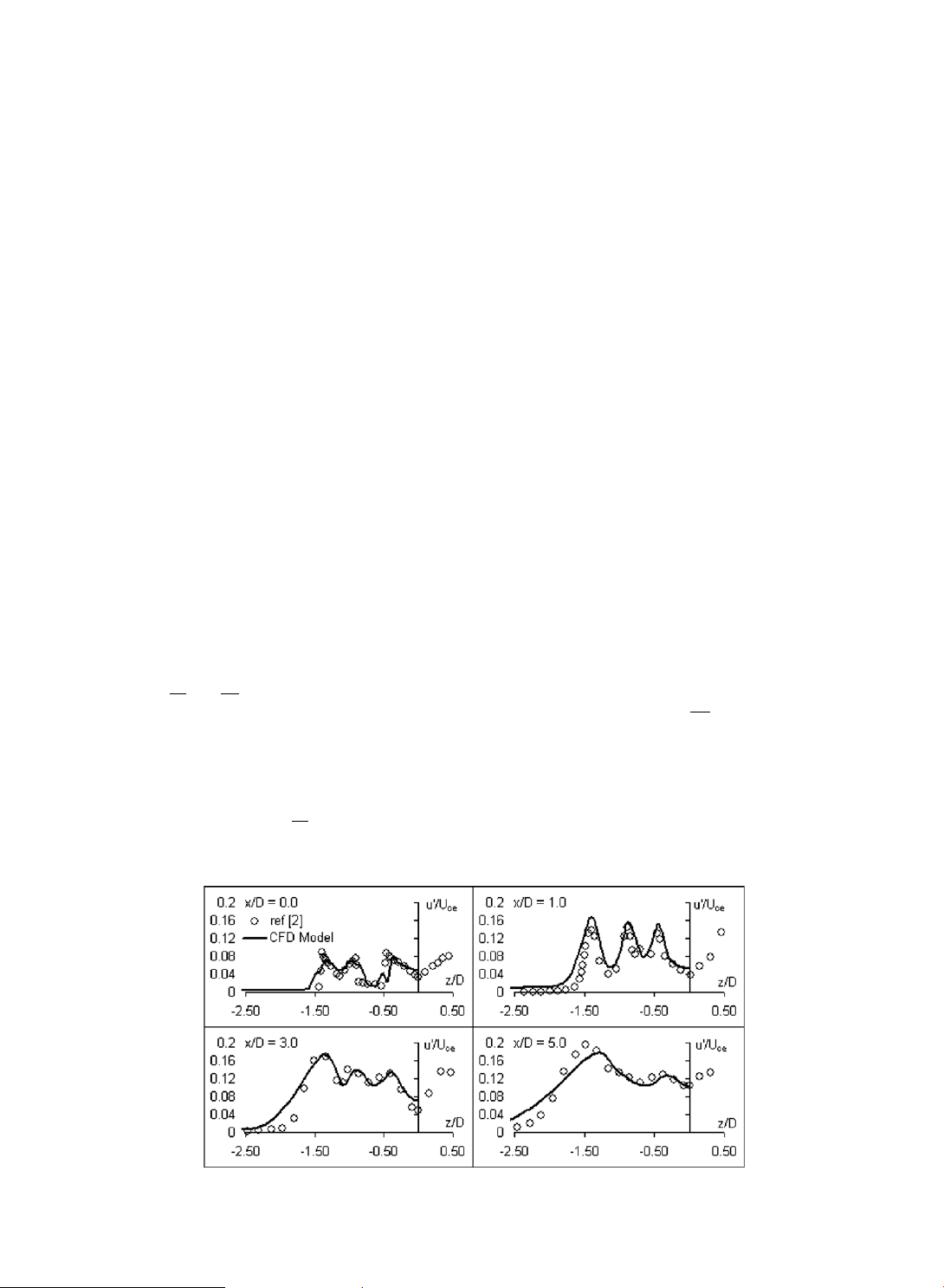
Hot-wire measurements of the turbulent velocity fluctuations in the xz plane at 9D from Ref. [2] are compared to the
square root of uu and vv normal stress predictions in Figs. 11 and 12 and with Reynolds shear stress predictions in Figs.
13 and 14. The w0 fluctuating velocity is not shown because it was very similar to v0, while the wv shear stress is not shown
because the magnitude was small and no experimental data was available.
The prediction of u0 matched the measured values closely at each location. At the burner exit plane u0 was non-zero at the
axis, which was also the case for Geometry A. This non-zero value occurred due to diffusive transport inwards from the re-
gion of peak generation in the cross-stream direction and from upstream. Peaks were found at the edges of the primary and secondary jets.
At 1D there was generation of uu in the shear layer but it had not yet diffused through the jet in the cross-stream direc-
tions because the minima at the centres of the secondary and primary jets were approximately the same magnitude as at the
Fig. 11. u0 turbulent velocity fluctuations – xz plane – Geometry B.
J.T. Hart et al. / Applied Mathematical Modelling 33 (2009) 3756–3767 3765
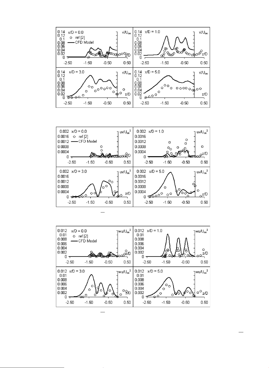
Fig. 12. v0 turbulent velocity fluctuations – xz plane – Geometry B.
Fig. 13. uv Reynolds stress profile – xz plane – Geometry B.
Fig. 14. uw Reynolds stress profile – xz plane – Geometry B.
exit plane. By 3D only the peak between the secondary jet and the free stream was maintained, which was in the region of
highest shear; the other two peaks actually decreased in magnitude. There appeared to be diffusive redistribution of uu in
this region, with the minima on the jet axes increasing and the peaks dropping in magnitude, leading to a more homoge- 3766
J.T. Hart et al. / Applied Mathematical Modelling 33 (2009) 3756–3767
neous stress distribution. At 5D there were only two peaks, one at the secondary jet boundary and another smaller peak at
the primary jet boundary. The profile between the secondary jet and surrounding fluid was not as steep in the prediction as
in the measurements, just as the gradient of the velocity profile was under-predicted in the same region.
The distributions of v0 and w0 were very similar, indicating that the turbulence was nearly isotropic in these directions.
Comparison of the predictions with the measurements showed similar profiles but the magnitude of the CFD model predic-
tion was almost double. In Ref. [1] the author comments on the cross-stream velocity data ‘‘due to small potential errors in
wire orientation angle, small deviations from the cosine law and shear gradient influences, little value can be obtained from
attempting a detailed interpretation of the cross-stream velocity data, particularly close to the outlet plane of the burner. As
the traverse plane is through the geometric centre of the three jets the mean cross-stream velocity normal to this plane, v,
should be close to zero. When the cross-wire was away from the influence of strong shear gradients, the results confirm this
is the case. Measurements of the cross-stream velocity component parallel to the traverse plane, w, are more difficult to interpret”.
The stress predictions for Geometry A were qualitatively validated against literature distributions for a plane jet and it
was found that the cross-stream fluctuations were around 70% of the stream-wise fluctuations in any given plane. These ra-
tios were similar in the predictions for Geometry B, v0/u0 approximately 0.7.
The Reynolds shear stresses were an order of magnitude less than the normal stresses; values of uv were a further order
of magnitude less than the uw stresses. The profile of uw was well matched; only the magnitudes disagreed. Very little cor-
relation was found for uv. Given these relatively small values and the associated uncertainty of the v0 and w0 measurements
the lack of agreement is not surprising, although it is not clear why it is manifested in one stress component and not the
other. Due to the small magnitude of the uv shear stress, there was little value in attempting to correlate the predictions
and measurements in any significant detail.
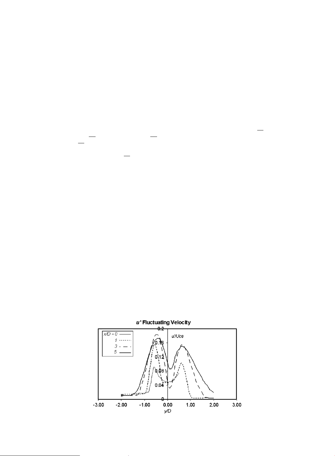
Shown in Fig. 15 is the fluctuating u0 velocity distribution on the xy plane through the centre of the primary jet at five
downstream locations; unfortunately there were no experimental measurements at these locations for comparison. Unlike
the velocity profiles the centre of these profiles corresponded to the geometric axis. Asymmetry was found in each profile
with higher values for each quantity found on the short side of the jet. The skew ness of the minima on the centre line
was caused, in part by the deviation of the jet from the geometric axis; however, part of the cause may also have been dif-
fusive transport from regions of high concentration such as the peak generation region in the shear layer. Because there was
more generation on the short side of the jet, it follows that it would be preferentially transported across the centreline to the
long side where the concentration was lower, which was the case. 5.3. Discussion of results
Numerical diffusion was significant in Geometry B where there was non-alignment of the grid with the mean flow direc-
tion. The extent of this problem was made apparent by comparing with Geometry A, which gave very accurate results with
only the hybrid-differencing scheme. It is a requirement then for such a higher order scheme to be used in all burner models
when the resulting flow is not aligned with the grid.
The RNG k–e model consistently predicted less dissipation of momentum in the jet compared to the other models as a
result of its lower turbulent viscosity calculation. This might have been an advantage except that it resulted in over-predic-
tion of centreline velocities in all cases in comparison to the physical model. Further investigation of the roots of this defi-
ciency might lead to improvements in the predictions. However, since the turbulence has been shown to be anisotropic this
bousinessq-based model will always lack an accurate description of the underlying turbulent physics. Thus any exact match-
Fig. 15. u0 turbulent velocity fluctuations – xz plane – Geometry B.
J.T. Hart et al. / Applied Mathematical Modelling 33 (2009) 3756–3767 3767
ing with the physical measurements by altering parameters in the model would be fortunate but might not be reliable for
other more complex flows and hence was not attempted in this study.
The flow field of Geometry B differed from that of Geometry A in that an internal pressure reorganization at the nozzle
resulted in a cross-stream pressure drop within the jet, which helped to bend the streamlines towards the long side resulting
in a slight deviation of the jets from their geometric centreline. A more detailed investigation of this phenomenon may yield
some interesting methods of controlling jet direction through manipulation of the pressure field at the nozzle.
Overall, the mean flow characteristics of the jets in Geometry B were very similar those in Geometry A. The nozzle angle
had little effect on jet centreline velocity decay, with both geometries showing almost the same decay rate, although Geom-
etry B was marginally higher. The only other differences were asymmetry in entrainment and stress distributions, which ap-
peared to have little effect on the mean flow. The quality of the flow field predictions using CFD modelling was good and this
result has increased confidence in CFD modelling for furnace flows. Acknowledgments
The authors gratefully acknowledge the financial support received for this research from the Cooperative Research Centre
(CRC) for Clean Power from Lignite, which is established and supported under the Australian Government’s Cooperative Re- search Centre’s program.
The authors would like to acknowledge the financial and other support of Swinburne University of Technology. References
[1] J.H. Perry, T. Hausler, Aerodynamics of Burner Jets Designed for Brown Coal Fired Boilers – Part III, SECV Report No. GO/83/57, State Electricity Commission of Victoria, 1982.
[2] J.H. Perry, T. Hausler, Aerodynamics of Burner Jets Designed for Brown Coal Fired Boilers – Part IV, SECV Report No. ND/84/004, State Electricity Commission of Victoria, 1984.
[3] W.P. Jones, B.E. Launder, The prediction of laminarisation with a two-equation model of turbulence, Int. J. Heat Mass Transfer 15 (1972) 301–314.
[4] V. Yakot, S.A. Orszag, Renormalization group analysis of turbulence: 1. Basic theory, J. Sci. Comput. 1 (1986) 3–51.
[5] B.E. Launder, G.J. Reece, W. Rodi, Progress in the developments of a Reynolds-stress turbulence closure, J. Fluid Mech. 68 (1975) 537–566.
[6] B.E. Launder, D.E. Spalding, The numerical computation of turbulent flows, Comput. Meth. Appl. Mech. Eng. 3 (1974) 269–289.
[7] J.H. Alderton, N.S. Wilkes, Some Application of New Finite Difference Schemes for Fluid Flow Problems, Report AERE-R 13234, Engineering Sciences
Division, Harwell Laboratory, Oxon, 1988.
[8] Suhas V. Patanker, Numerical Heat Transfer and Fluid Flow, Hemisphere Publishing Corporation, Washington, DC, 1980.
[9] C.M. Rhie, W.L. Chow, Numerical study of flow past an airfoil with trailing edge separation, AIAA J. 21 (11) (1983) 1525–1532.
[10] F.P. Ricou, D.V. Spalding, Measurements of entrainment by axisymmetric turbulent jets, J. Fluid Mech. 11 (1961) 21.
[11] D.R. Miller, E.W. Comings, Force momentum fields in a dual jet flow, J. Fluid Mech. 7 (1960) 237–256.
[12] P. Bradshaw, Turbulence Modelling Course – Lecture Notes, Imperial College, London, 1987.
[13] H. Elbanna, S. Gahin, M.I.I. Rashed, Investigation of two plane parallel jets, AIAA J. 21 (7) (1983) 986–991.
[14] A. Pollard, M.A. Iwaniw, Flow from sharp-edged rectangular orifices – the effect of corner rounding, AIAA J. 23 (4) (1985) 631–633.
[15] A. Krothapalli, D. Baganoff, K. Karamcheti, On mixing of a rectangular jet, J. Fluid Mech. 107 (1981) 201–220.
[16] W.R. Quinn, Stream-wise evolution of a square jet cross section, AIAA J. 30 (12) (1992) 2853–2857.
[17] B. Massey, Mechanics of Fluids, seventh ed., Stanley Thornes Ltd., United Kingdom, 1998.
Document Outline

• Aerodynamics of an isolated slot-burner from a tangentially-fired boiler
  • Introduction
  • Numerical models and procedures used
  • Model geometry and boundary conditions
  • Grids and grid dependence
  • Results and discussion
    • Geometry A – orthogonal Jets
    • Geometry B – angled Jets
      • Flow field prediction
      • Comparison with experiment
    • Discussion of results
  • Acknowledgments
  • References