

Bài giảng 6 chương 4: Differentiation | Môn kinh tế vi mô

Supply is said to be inelastic if E < 1, unit elastic if E = 1 and elastic if E > 1Arc elasticity E (for arc of the supply curve from point (P1, Q1) to (P2, Q2)  is calculated as above,  where Q is replaced by (Q1 + Q2)/2 & P by (P1 + P2)/2. Tài liệu giúp bạn tham khảo, ôn tập và đạt kết quả cao. Mời bạn đọc đón xem !

Môn:
Thông tin:
15 trang 1 tháng trước

Bình luận

Vui lòng đăng nhập hoặc đăng ký để gửi bình luận.

Bài giảng 6 chương 4: Differentiation | Môn kinh tế vi mô

Supply is said to be inelastic if E < 1, unit elastic if E = 1 and elastic if E > 1Arc elasticity E (for arc of the supply curve from point (P1, Q1) to (P2, Q2)  is calculated as above,  where Q is replaced by (Q1 + Q2)/2 & P by (P1 + P2)/2. Tài liệu giúp bạn tham khảo, ôn tập và đạt kết quả cao. Mời bạn đọc đón xem !

42 21 lượt tải Tải xuống
lOMoARcPSD| 47207194 7/31/2020
1
Jacques,
Mathematics for Economics and Business
, 7
th
edition © Pearson Education Limited 2012
Slide 4.1
Lecture 6
(31/03/2020)
Chapter 4 (contd.)
Differentiation
Section 4.5. Elasticity Sections 4.6 and 4.7. Optimization
of economic functions
Section 4.8. The derivatives of exponential and natural
logarithm functions
Jacques, Mathematics for Economics and Business , 7
th
edition © Pearson Education Limited 2012
Slide 4.2
Section 4.5. Elasticity
Price elasticity of demand and of supply
The relationship between price elasticity of demand
and marginal revenue
Price elasticity for general linear demand functions.
Slide 4.3
lOMoARcPSD| 47207194 7/31/2020
2
Jacques,
Mathematics for Economics and Business
, 7
th
edition © Pearson Education Limited 2012
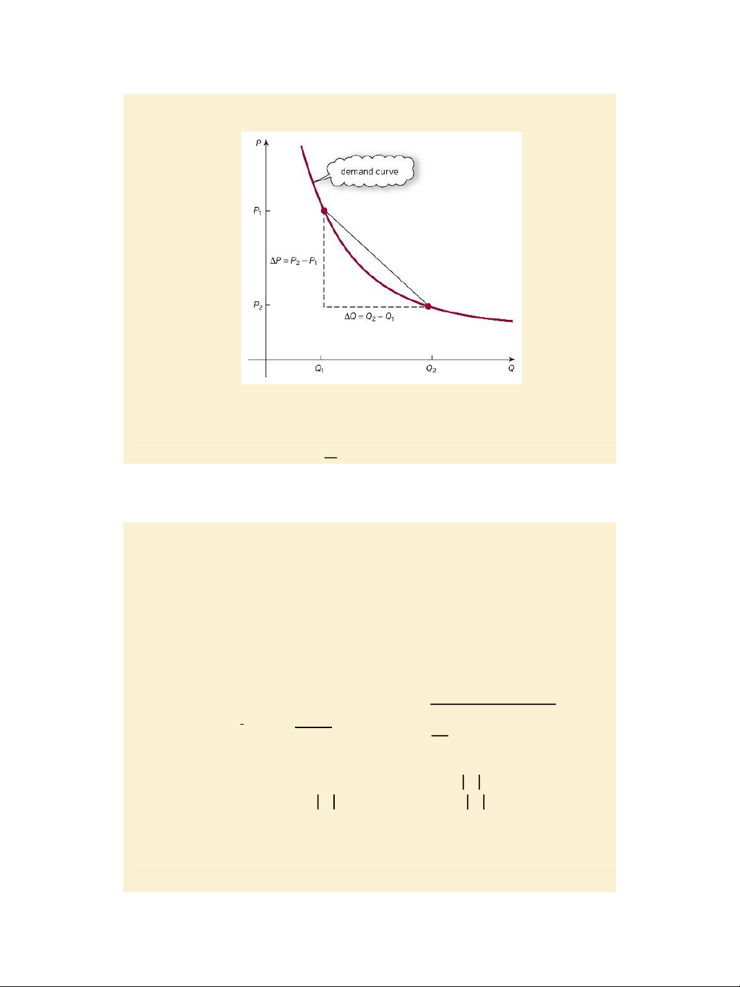
Figure 4.17
The demand curve
Δ𝑄
< 0 Page 316
Δ𝑃
Jacques, Mathematics for Economics and Business , 7
th
edition © Pearson Education Limited 2012
Slide 4.4
Price elasticity of demand
Price elasticity of demand E==
% 𝒄𝒉𝒂𝒏𝒈𝒆 𝒊𝒏 𝒅𝒆𝒎𝒂𝒏𝒅
% 𝒄𝒉𝒂𝒏𝒈𝒆 𝒊𝒏 𝒑𝒓𝒊𝒄𝒆
∆𝑸/𝑸 = ∆𝑸/∆𝑷 < 0 since Δ𝑄 < 0.
∆𝑷/𝑷 𝑸/𝑷 Δ𝑃
Demand is said to be inelastic if 𝐸 < 1, unit
elastic if 𝐸 = 1 and elastic if 𝐸 > 1.
Arc elasticity E (for arc of the demand curve from point
lOMoARcPSD| 47207194 7/31/2020
3
Jacques,
Mathematics for Economics and Business
, 7
th
edition © Pearson Education Limited 2012
(P
1
, Q
1
) to (P
2
, Q
2
) is calculated as above, where Q
is replaced by (Q
1
+ Q
2
)/2 & P by (P
1
+ P
2
)/2
Point elasticity E =
𝒅𝑸/𝒅𝑷
, with
d𝑄
< 0.
𝑸/𝑷 dP
Example and practice problem pages 315 – 318
Slide 4.5
The derivative of an inverse function
Q = g(P) P = f(Q)
𝒅𝑸 𝟏 =
𝒅𝑷 𝒅𝑷/𝒅𝑸
Example and practice problem pages 319 - 320
Given the demand function: P = -Q
2
– 4Q +96
Calculate dQ/dP at P = 51
From P = 51 one can derive Q = 5.
At Q = 5, dP/dQ = -2Q – 4 = -14
Hence dQ/dP = -1/14 and E = =
𝒅𝑸/𝒅𝑷
= - = - 0.73
𝑸/𝑷
Jacques,
Mathematics for Economics and Business, 7
th
edition © Pearson Education Limited
2012
Slide 4.6
Price elasticity of supply Price elasticity of supply
E=
% 𝒄𝒉𝒂𝒏𝒈𝒆 𝒊𝒏 𝒔𝒖𝒑𝒑𝒍𝒚
% 𝒄𝒉𝒂𝒏𝒈𝒆 𝒊𝒏 𝒑𝒓𝒊𝒄𝒆
= ∆𝑸/𝑸 = ∆𝑸/∆𝑷 > 0 since Δ𝑄 > 0.
∆𝑷/𝑷 𝑸/𝑷 Δ𝑃
lOMoARcPSD| 47207194 7/31/2020
4
Jacques,
Mathematics for Economics and Business
, 7
th
edition © Pearson Education Limited 2012
Supply is said to be inelastic if E < 1, unit elastic if E = 1
and elastic if E > 1.
Arc elasticity E (for arc of the supply curve from point (P
1
,
Q
1
) to (P
2
, Q
2
) is calculated as above, where Q is
replaced by (Q
1
+ Q
2
)/2 & P by (P
1
+ P
2
)/2
Point elasticity E =
𝒅𝑸/𝒅𝑷
, with
d𝑄
> 0.
𝑸/𝑷 d𝑃
Example and practice problem pages 321 – 323
Slide 4.7
The relationship between price elasticity of demand
and marginal revenue
Marginal revenue MR =
𝑑 𝑇𝑅
=
𝑑(𝑃𝑄)
= 𝑃 + 𝑄 ×
𝑑𝑃
=
𝑑𝑄 𝑑𝑄 𝑑𝑄
𝑃 1 +
𝑑𝑃/𝑑𝑄
= 𝑃 1 +
1
where E < 0
𝑃/𝑄 𝐸
MR negative if E > -1, MR = 0 if E =-1, MR positive if E< -1.
Price elasticity for a linear demand function P
= aQ + b with a < 0 and b > 0.
1
Hence E = 𝒅𝑸/𝒅𝑷 = 𝑎 =
𝑃 𝑸/𝑷
𝑎
1
𝑃−𝑏
𝑃−𝑏
𝑃
E depends on b only and is independent of slope a
pages 322 – 323
lOMoARcPSD| 47207194 7/31/2020
5
Jacques,
Mathematics for Economics and Business
, 7
th
edition © Pearson Education Limited 2012
Jacques, Mathematics for Economics and Business , 7
th
edition © Pearson Education Limited
2012 Slide 4.8
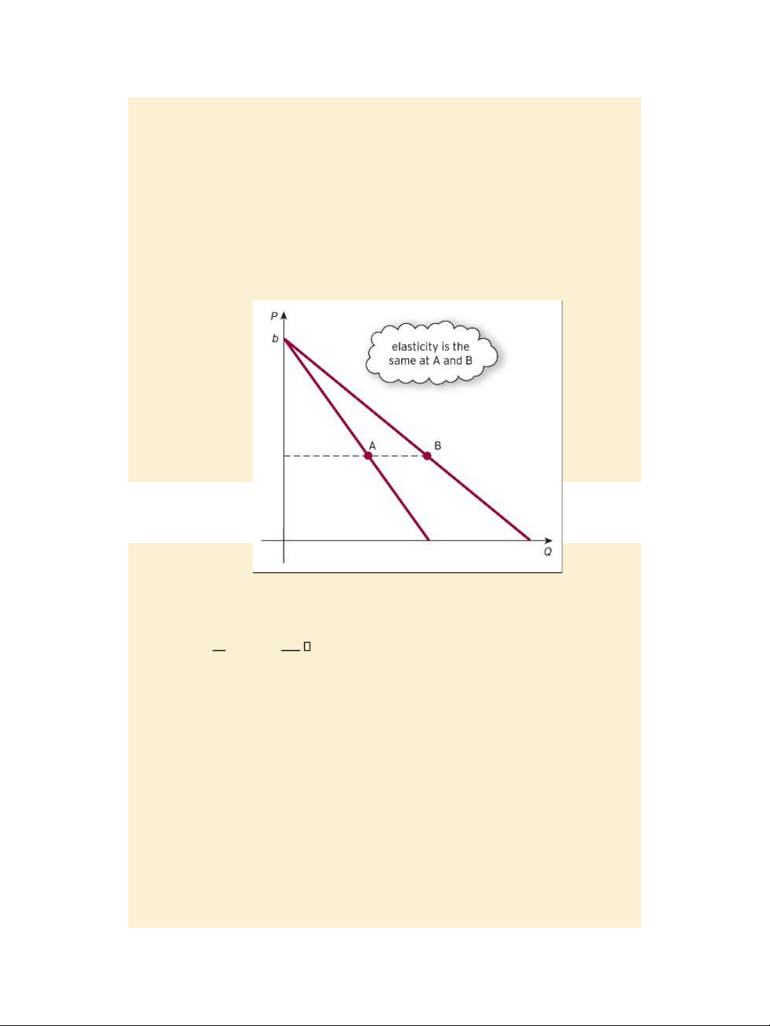
Figure 4.18 page 295
The linear demand curve
Δ𝑄 𝑃
< 0 , E= E is the same at A & B (b and P are the same),
Δ𝑃 𝑃−𝑏
Page 324
Slide 4.9
lOMoARcPSD| 47207194 7/31/2020
6
Jacques,
Mathematics for Economics and Business
, 7
th
edition © Pearson Education Limited 2012
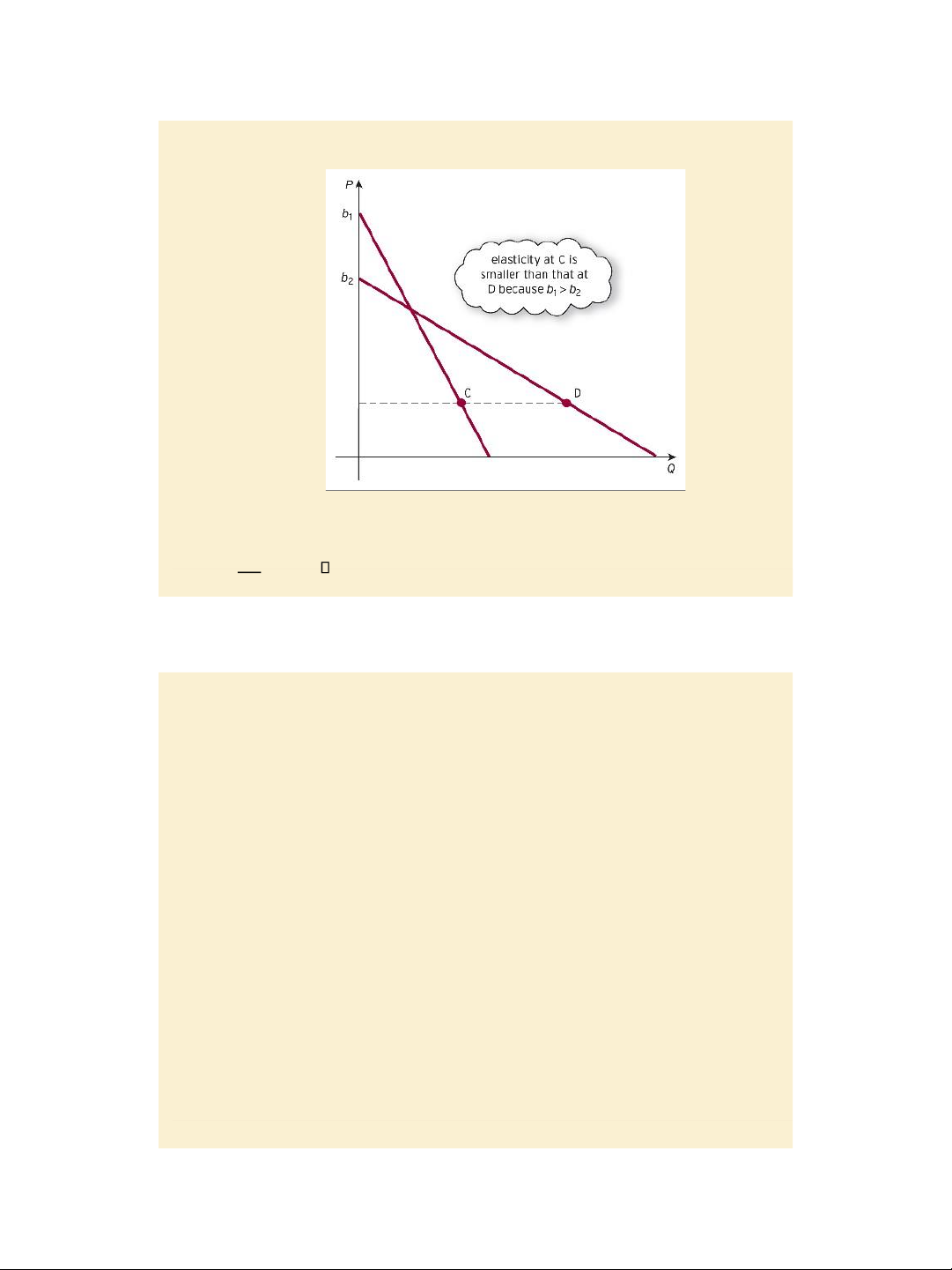
Figure 4.19
The linear demand curve
E= 𝑃−𝑏
𝑃
< 0 E at C > E at D for the same P and for b
1
> b
2
, page 324
Key terms: page 326, Exercise 4.5*: problems 3, 4, 6, 7 page
327
Jacques, Mathematics for Economics and Business , 7
th
edition © Pearson Education Limited 2012
Slide 4.10
lOMoARcPSD| 47207194 7/31/2020
7
Jacques,
Mathematics for Economics and Business
, 7
th
edition © Pearson Education Limited 2012
𝑃−𝑏
Slide 4.11
Section 4.6. Optimization
Using 1st order and 2nd order derivatives to classify stationary points,
finding maximum and minimum points,
and
optimizing economic functions
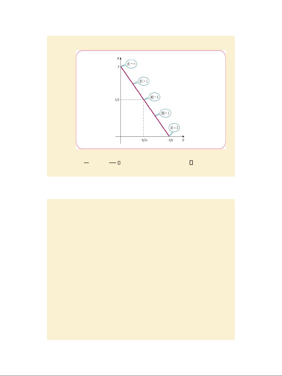
Figure 4.20
Δ𝑄
Δ𝑃
< 0 , E=
𝑃
E = 0 for P = 0 and E tends to -
for P =b
E = 1 when P = b/2 ( or Q = -b/(2a) ) Page 325
lOMoARcPSD| 47207194 7/31/2020
8
Jacques,
Mathematics for Economics and Business
, 7
th
edition © Pearson Education Limited 2012
Jacques, Mathematics for Economics and Business , 7
th
edition © Pearson Education Limited 2012
Slide 4.12
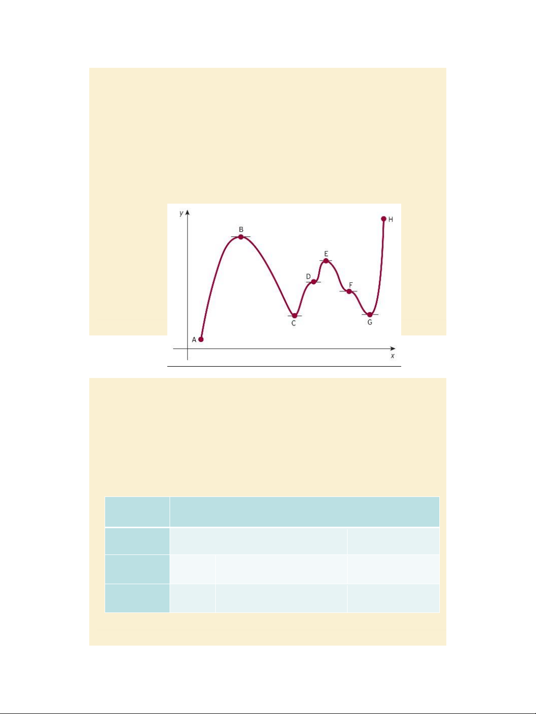
Figure 4.21
Discussion on stationary (critical, turning) points, local
(relative) maximum & minimum (extrema)
Pages 329 - 331
Slide 4.13
Classification of stationary points
f’(a)= 0
Stationary
point
f’(a) = 0
Sign of f’
Sign of f’’
Minimum
point
f’(a) = 0,
f’(x) < 0 for x < a
f’(x) > 0 for x > a
f’’(a) > 0
Maximum
point
f’(a) = 0,
f’(x) > 0 for x < a
f’(x) < 0 for x > a
f’’(a) < 0
lOMoARcPSD| 47207194 7/31/2020
9
Jacques,
Mathematics for Economics and Business
, 7
th
edition © Pearson Education Limited 2012
Reflection
point
f’(a) = 0,
f’(x) < 0 for x < a and x > a
or
f’(x) > 0 for x < a and x > a
f’’(x) < 0 for x < a
f’’(x) > 0 for x > a
or
f’’(x) > 0 for x < a
f’’(x) < 0 for x > a
Jacques, Mathematics for Economics and Business , 7
th
edition © Pearson Education Limited 2012
Slide 4.14
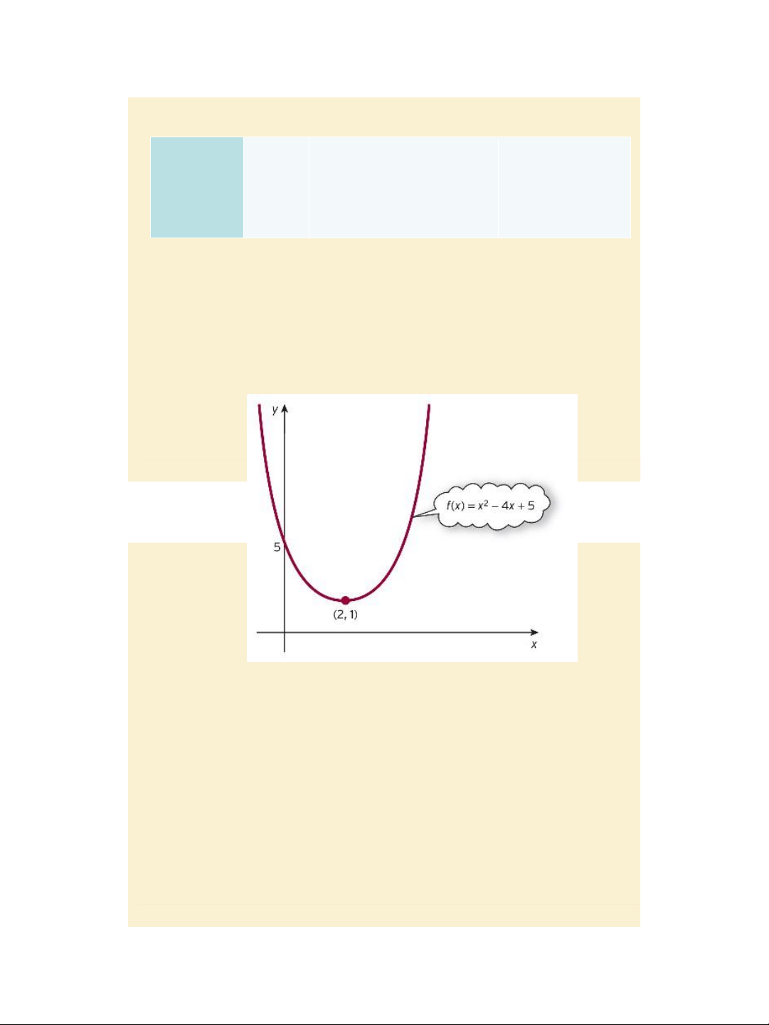
Figure 4.22
Find and classify stationary points
Example pages 331 - 332
Slide 4.15
lOMoARcPSD| 47207194 7/31/2020
10
Jacques,
Mathematics for Economics and Business
, 7
th
edition © Pearson Education Limited 2012
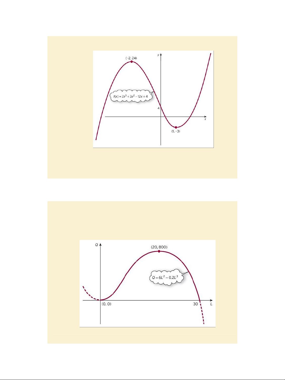
Figure 4.24
Find and classify stationary points
Example and practice problem pages
332 - 335
Jacques, Mathematics for Economics and Business , 7
th
edition © Pearson Education Limited 2012
Slide 4.16
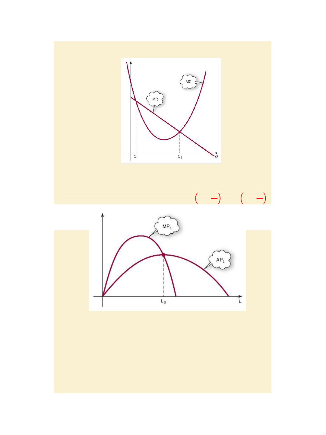
Figure 4.25
lOMoARcPSD| 47207194 7/31/2020
11
Jacques,
Mathematics for Economics and Business
, 7
th
edition © Pearson Education Limited 2012
Optimizing production function: Maximizing output Q
and average product of labor AP
L
(or labor productivity)
Example and practice problem pages 335 –338:
Labor productivity max iff AP
L
= MP
L
Slide 4.17
Section 4.7. Further optimization of
economic functions
Maximizing total revenue and profit functions (example and
practice problem pages 338-340: profit max iff MR = MC)
Minimizing the average cost function (example and practice
problem pages 341-342: AC = MC)
Maximizing the government’s total tax revenue (example
and practice problem pages 343-344)
Key terms: page 345.
Exercise 4.6*: problems 1, 3, 6 page 347
Jacques, Mathematics for Economics and Business, 7
th
edition © Pearson Education Limited
2012 Slide 4.18
lOMoARcPSD| 47207194 7/31/2020
12
Jacques,
Mathematics for Economics and Business
, 7
th
edition © Pearson Education Limited 2012
Figure 4.26
Profit is maximized iff MR = MC, Proof: pages 348 – 349
Example and practice problems, pages 350 – 354.
Profit is maximized iff MR
1
= MR
2
or 𝑷
𝟏
𝟏 +
𝑬
𝟏
𝟏 = 𝑷
𝟐
𝟏 +
𝑬
𝟏
𝟐
Slide 4.19
Figure 4.27
Labor productivity AP
L
is maximized iff MP
L
= AP
L
,
Proof: pages 355 – 356, Exercise
4.7*: problems 1, 2, 3, 5, page 359.
Jacques, Mathematics for Economics and Business , 7
th
edition © Pearson Education Limited 2012
lOMoARcPSD| 47207194 7/31/2020
13
Jacques,
Mathematics for Economics and Business
, 7
th
edition © Pearson Education Limited 2012
Slide 4.20
Section 4.8. The derivatives of the
exponential and natural logarithm
functions
Differentiate the exponential and natural logarithm functions and their
combinations
and
Some applications of the exponential and natural
logarithm functions in economics
Slide 4.21
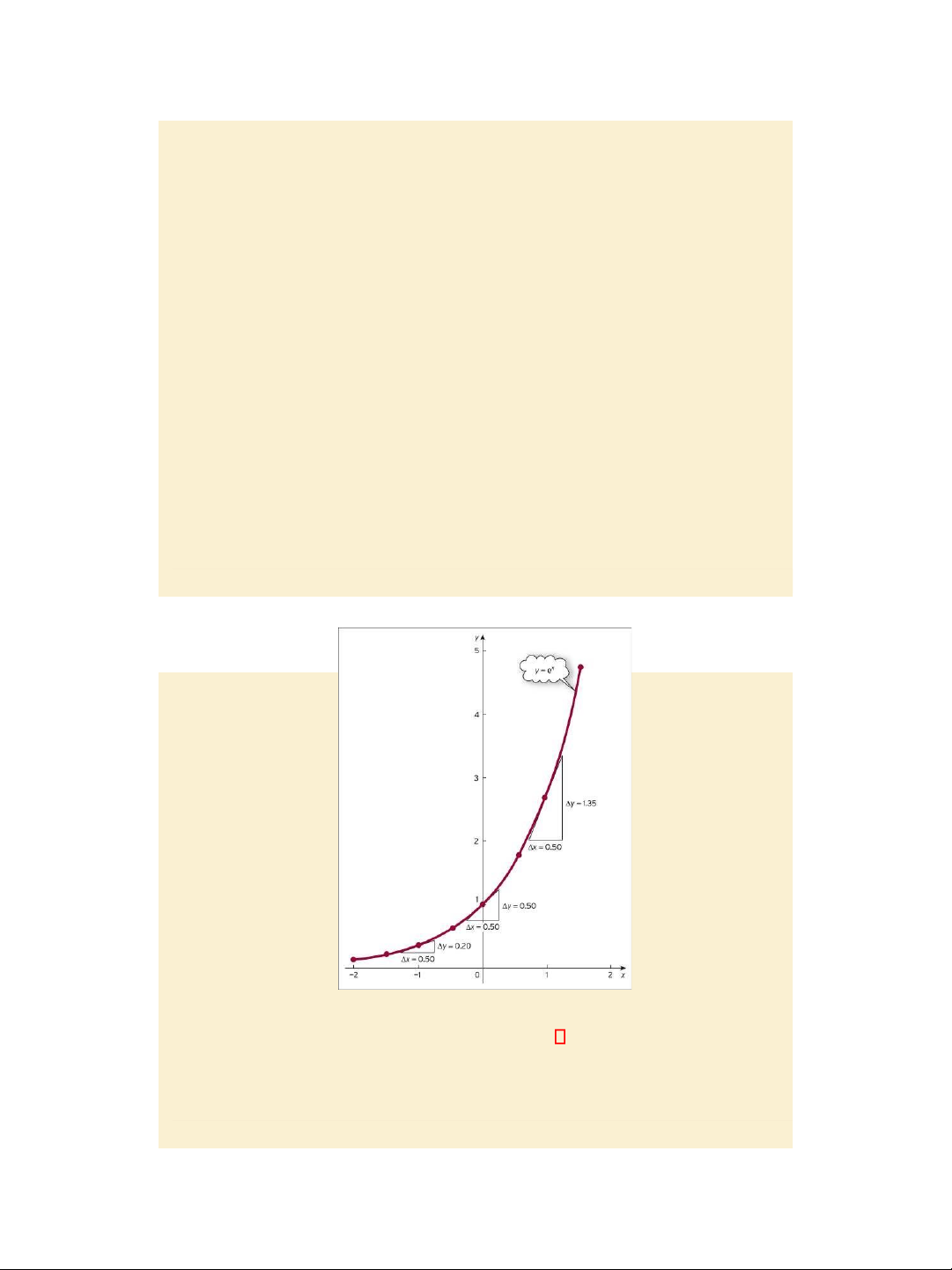
Figure 4.30
Exponential function: y = e
x
y’ = e
x
Example:
pages 361 – 362.
Jacques, Mathematics for Economics and Business , 7
th
edition © Pearson Education Limited 2012
lOMoARcPSD| 47207194 7/31/2020
14
Jacques,
Mathematics for Economics and Business
, 7
th
edition © Pearson Education Limited 2012
Slide 4.22
The natural logarithm function:
y = 𝒍𝒏𝒙 ⟹ 𝒚
=
𝟏
𝒙
practice problem: page 363
y = 𝒆
𝒎𝒙
𝒚
= 𝒎𝒆
𝒎𝒙
y =
𝒍𝒏(𝒎𝒙) ⟹ 𝒚
=
𝟏
𝒙
proof: use the chain rule, page 363
Examples and practice problems, pages 363 -366
Applications of exponential and natural logarithm
functions in economics
Examples and practice problems, pages 367 -369
Exercise 4.8*: problems 1, 2, 7, 8, 9 pages 371 – 372.
Slide 4.23
Figure 4.31 and 4.32
lOMoARcPSD| 47207194 7/31/2020
15
Jacques,
Mathematics for Economics and Business
, 7
th
edition © Pearson Education Limited 2012
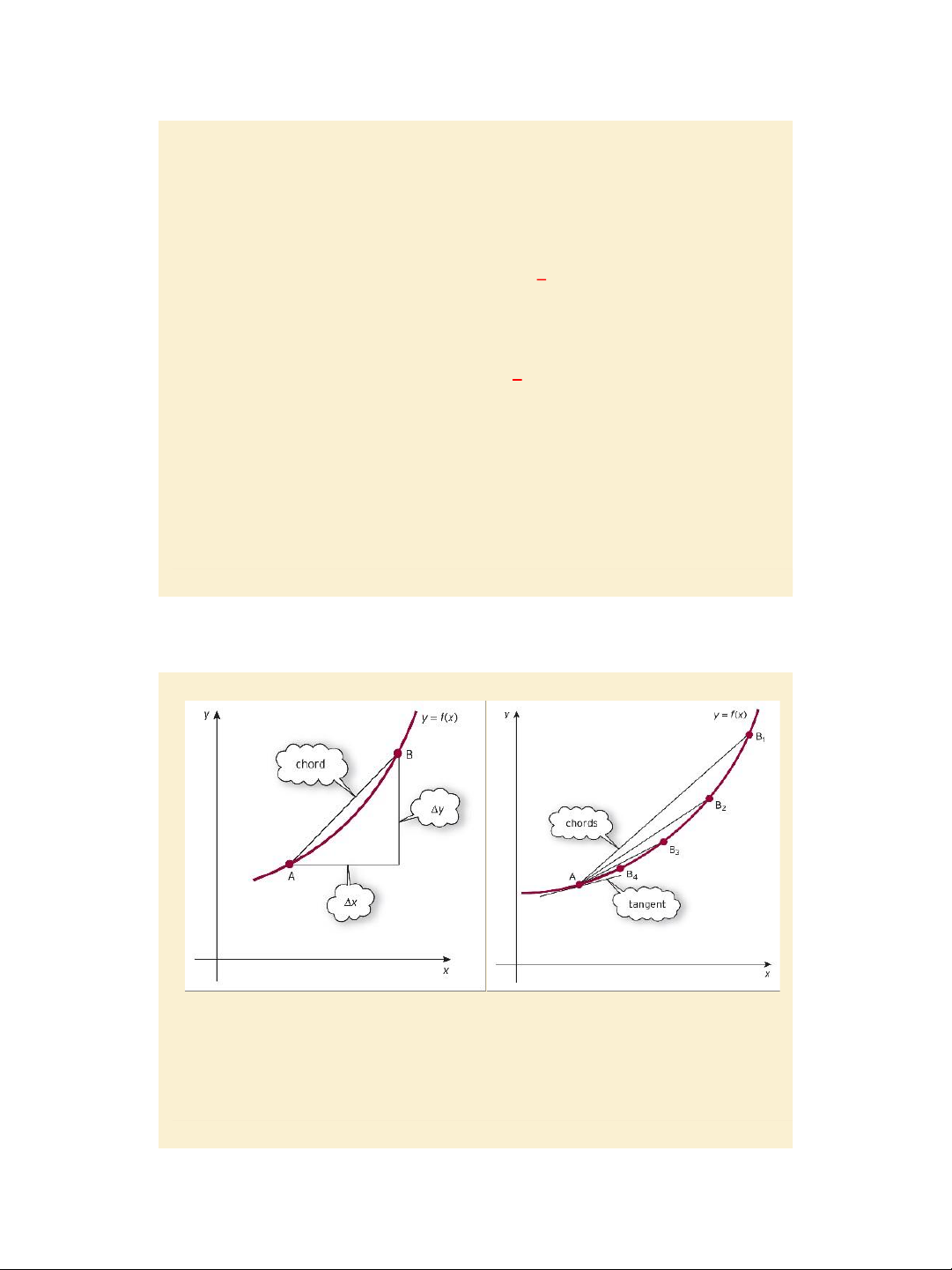
Formal mathematics:
𝒅𝒚
= lim
𝚫𝒚
𝒅𝒙 𝚫𝑥0 𝚫𝒙
Pages 373 – 374.
Jacques, Mathematics for Economics and Business , 7
th
edition © Pearson Education Limited 2012
Slide 4.24
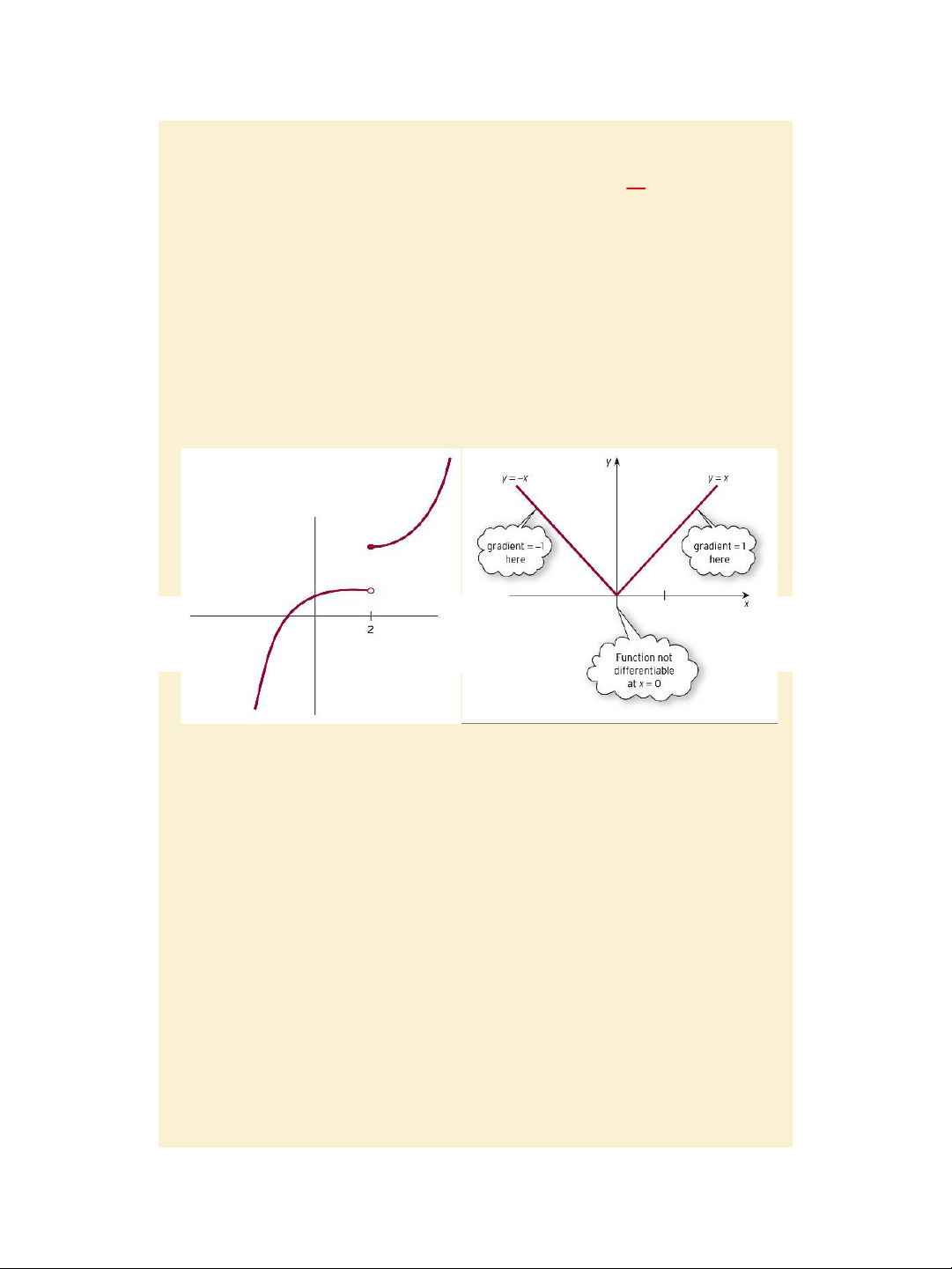
Figure 4.33 and 4.34
Formal mathematics: points at which
functions are not differentiable Pages
374 – 375.
| 1/15

Preview text:

7/31/2020 lOMoAR cPSD| 47207194 Slide 4.1 Lecture 6 (31/03/2020) Chapter 4 (contd.) Differentiation
Section 4.5. Elasticity Sections 4.6 and 4.7. Optimization of economic functions
• Section 4.8. The derivatives of exponential and natural logarithm functions
Jacques, Mathematics for Economics and Business, 7th edition © Pearson Education Limited 2012 Slide 4.2 Section 4.5. Elasticity
Price elasticity of demand and of supply
The relationship between price elasticity of demand and marginal revenue
Price elasticity for general linear demand functions. Slide 4.3
Jacques, Mathematics for Economics and Business , 7 th edition © Pearson Education Limited 2012 1 7/31/2020 lOMoAR cPSD| 47207194 Figure 4.17 The demand curve Δ𝑄 < 0 Page 316 Δ𝑃
Jacques, Mathematics for Economics and Business, 7th edition © Pearson Education Limited 2012 Slide 4.4
Price elasticity of demand
Price elasticity of demand E== % 𝒄𝒉𝒂𝒏𝒈𝒆 𝒊𝒏 𝒅𝒆𝒎𝒂𝒏𝒅
% 𝒄𝒉𝒂𝒏𝒈𝒆 𝒊𝒏 𝒑𝒓𝒊𝒄𝒆 ∆𝑸/𝑸 =
∆𝑸/∆𝑷 < 0 since Δ𝑄 < 0. ∆𝑷/𝑷 𝑸/𝑷 Δ𝑃
Demand is said to be inelastic if 𝐸 < 1, unit
elastic if 𝐸 = 1 and elastic if 𝐸 > 1.
Arc elasticity E (for arc of the demand curve from point
Jacques, Mathematics for Economics and Business , 7 th edition © Pearson Education Limited 2012 2 7/31/2020 lOMoAR cPSD| 47207194
(P1, Q1) to (P2, Q2) is calculated as above, where Q
is replaced by (Q1 + Q2)/2 & P by (P1 + P2)/2
Point elasticity E =
𝒅𝑸/𝒅𝑷 , with d𝑄 < 0. 𝑸/𝑷 dP
Example and practice problem pages 315 – 318 Slide 4.5
The derivative of an inverse function Q = g(P) P = f(Q) 𝒅𝑸 𝟏 = 𝒅𝑷 𝒅𝑷/𝒅𝑸
Example and practice problem pages 319 - 320
Given the demand function: P = -Q2 – 4Q +96 Calculate dQ/dP at P = 51
From P = 51 one can derive Q = 5.
At Q = 5, dP/dQ = -2Q – 4 = -14 Hence dQ/dP = -1/14 and E = = 𝒅𝑸/𝒅𝑷 = - = - 0.73 𝑸/𝑷
Jacques, Mathematics for Economics and Business, 7th edition © Pearson Education Limited 2012 Slide 4.6
Price elasticity of supply Price elasticity of supply
E= % 𝒄𝒉𝒂𝒏𝒈𝒆 𝒊𝒏 𝒔𝒖𝒑𝒑𝒍𝒚
% 𝒄𝒉𝒂𝒏𝒈𝒆 𝒊𝒏 𝒑𝒓𝒊𝒄𝒆
= ∆𝑸/𝑸 =
∆𝑸/∆𝑷 > 0 since Δ𝑄 > 0. ∆𝑷/𝑷 𝑸/𝑷 Δ𝑃
Jacques, Mathematics for Economics and Business , 7 th edition © Pearson Education Limited 2012 3 7/31/2020 lOMoAR cPSD| 47207194
Supply is said to be inelastic if E < 1, unit elastic if E = 1 and elastic if E > 1.
Arc elasticity E (for arc of the supply curve from point (P1,
Q1) to (P2, Q2) is calculated as above, where Q is
replaced by (Q1 + Q2)/2 & P by (P1 + P2)/2
Point elasticity E =
𝒅𝑸/𝒅𝑷 , with d𝑄 > 0. 𝑸/𝑷 d𝑃
Example and practice problem pages 321 – 323 Slide 4.7
The relationship between price elasticity of demand and marginal revenue
Marginal revenue MR = 𝑑 𝑇𝑅 = 𝑑(𝑃𝑄) = 𝑃 + 𝑄 × 𝑑𝑃 = 𝑑𝑄 𝑑𝑄 𝑑𝑄
𝑃 1 + 𝑑𝑃/𝑑𝑄 = 𝑃 1 + 1 where E < 0 𝑃/𝑄 𝐸
MR negative if E > -1, MR = 0 if E =-1, MR positive if E< -1.
Price elasticity for a linear demand function P
= aQ + b with a < 0 and b > 0. 1 Hence E = 𝒅𝑸/𝒅𝑷 = 𝑎 =
𝑃 𝑸/𝑷 𝑎1 𝑃−𝑏 𝑃−𝑏 𝑃
E depends on b only and is independent of slope a pages 322 – 323
Jacques, Mathematics for Economics and Business , 7 th edition © Pearson Education Limited 2012 4 7/31/2020 lOMoAR cPSD| 47207194
Jacques, Mathematics for Economics and Business, 7th edition © Pearson Education Limited 2012 Slide 4.8 Figure 4.18 page 295
The linear demand curve Δ𝑄 𝑃 < 0 , E=
E is the same at A & B (b and P are the same), Δ𝑃 𝑃−𝑏 Page 324 Slide 4.9
Jacques, Mathematics for Economics and Business , 7 th edition © Pearson Education Limited 2012 5 7/31/2020 lOMoAR cPSD| 47207194 Figure 4.19
The linear demand curve E=
𝑃−𝑏𝑃 < 0 E at C > E at D for the same P and for b1 > b2 , page 324
Key terms: page 326, Exercise 4.5*: problems 3, 4, 6, 7 page 327
Jacques, Mathematics for Economics and Business, 7th edition © Pearson Education Limited 2012 Slide 4.10
Jacques, Mathematics for Economics and Business , 7 th edition © Pearson Education Limited 2012 6 7/31/2020 lOMoAR cPSD| 47207194 Figure 4.20
The linear demand curve Δ𝑄
Δ𝑃 < 0 , E= 𝑃 E = 0 for P = 0 and E tends to - for P =b
E = 1 when P = b/2 ( or Q = -b/(2a) ) Page 325 𝑃−𝑏 Slide 4.11 Section 4.6. Optimization
Using 1st order and 2nd order derivatives to classify stationary points,
finding maximum and minimum points, and
optimizing economic functions
Jacques, Mathematics for Economics and Business , 7 th edition © Pearson Education Limited 2012 7 7/31/2020 lOMoAR cPSD| 47207194
Jacques, Mathematics for Economics and Business, 7th edition © Pearson Education Limited 2012 Slide 4.12 Figure 4.21
Discussion on stationary (critical, turning) points, local
(relative) maximum & minimum (extrema) Pages 329 - 331 Slide 4.13
Classification of stationary points f’(a)= 0 Stationary f’(a) = 0 point Sign of f’ Sign of f’’ Minimum
f’(a) = 0, f’(x) < 0 for x < a f’ (a) > 0 point f’(x) > 0 for x > a Maximum
f’(a) = 0, f’(x) > 0 for x < a f’ (a) < 0 point f’(x) < 0 for x > a
Jacques, Mathematics for Economics and Business , 7 th edition © Pearson Education Limited 2012 8 7/31/2020 lOMoAR cPSD| 47207194 Reflection
f’(a) = 0, f’(x) < 0 for x < a and x > a f’ (x) < 0 for x < a point or f’ (x) > 0 for x > a
f’(x) > 0 for x < a and x > a or f’ (x) > 0 for x < a f’ (x) < 0 for x > a
Jacques, Mathematics for Economics and Business, 7th edition © Pearson Education Limited 2012 Slide 4.14 Figure 4.22
Find and classify stationary points Example pages 331 - 332 Slide 4.15
Jacques, Mathematics for Economics and Business , 7 th edition © Pearson Education Limited 2012 9 7/31/2020 lOMoAR cPSD| 47207194 Figure 4.24
Find and classify stationary points
Example and practice problem pages 332 - 335
Jacques, Mathematics for Economics and Business, 7th edition © Pearson Education Limited 2012 Slide 4.16 Figure 4.25
Jacques, Mathematics for Economics and Business , 7 th edition © Pearson Education Limited 2012 10 7/31/2020 lOMoAR cPSD| 47207194
Optimizing production function: Maximizing output Q
and average product of labor APL (or labor productivity)
Example and practice problem pages 335 –338:
Labor productivity max iff APL = MPL Slide 4.17
Section 4.7. Further optimization of economic functions
Maximizing total revenue and profit functions (example and
practice problem pages 338-340: profit max iff MR = MC)
Minimizing the average cost function (example and practice
problem pages 341-342: AC = MC)
Maximizing the government’s total tax revenue (example
and practice problem pages 343-344) Key terms: page 345.
Exercise 4.6*: problems 1, 3, 6 page 347 Jacques,
Mathematics for Economics and Business, 7th edition © Pearson Education Limited 2012 Slide 4.18
Jacques, Mathematics for Economics and Business , 7 th edition © Pearson Education Limited 2012 11 7/31/2020 lOMoAR cPSD| 47207194 Figure 4.26
Profit is maximized iff MR = MC, Proof: pages 348 – 349
Example and practice problems, pages 350 – 354.
Profit is maximized iff MR1 = MR2 or 𝑷𝟏
𝟏 + 𝑬𝟏𝟏 = 𝑷𝟐 𝟏 + 𝑬𝟏𝟐 Slide 4.19 Figure 4.27
Labor productivity APL is maximized iff MPL = APL,
Proof: pages 355 – 356, Exercise
4.7*: problems 1, 2, 3, 5, page 359.
Jacques, Mathematics for Economics and Business, 7th edition © Pearson Education Limited 2012
Jacques, Mathematics for Economics and Business , 7 th edition © Pearson Education Limited 2012 12 7/31/2020 lOMoAR cPSD| 47207194 Slide 4.20
Section 4.8. The derivatives of the
exponential and natural logarithm functions
Differentiate the exponential and natural logarithm functions and their combinations and
Some applications of the exponential and natural
logarithm functions in economics Slide 4.21 Figure 4.30
Exponential function: y = ex y’ = ex Example: pages 361 – 362.
Jacques, Mathematics for Economics and Business, 7th edition © Pearson Education Limited 2012
Jacques, Mathematics for Economics and Business , 7 th edition © Pearson Education Limited 2012 13 7/31/2020 lOMoAR cPSD| 47207194 Slide 4.22
The natural logarithm function:
y = 𝒍𝒏𝒙 ⟹ 𝒚′ = 𝟏 𝒙 practice problem: page 363
y = 𝒆𝒎𝒙 ⟹ 𝒚′ = 𝒎𝒆𝒎𝒙 y =
𝒍𝒏(𝒎𝒙) ⟹ 𝒚′ = 𝟏 𝒙
proof: use the chain rule, page 363
Examples and practice problems, pages 363 -366
Applications of exponential and natural logarithm functions in economics
Examples and practice problems, pages 367 -369
Exercise 4.8*: problems 1, 2, 7, 8, 9 pages 371 – 372. Slide 4.23 Figure 4.31 and 4.32
Jacques, Mathematics for Economics and Business , 7 th edition © Pearson Education Limited 2012 14 7/31/2020 lOMoAR cPSD| 47207194
Formal mathematics: 𝒅𝒚 = lim 𝚫𝒚 𝒅𝒙 𝚫𝑥⇢0 𝚫𝒙 Pages 373 – 374.
Jacques, Mathematics for Economics and Business, 7th edition © Pearson Education Limited 2012 Slide 4.24 Figure 4.33 and 4.34
Formal mathematics: points at which
functions are not differentiable Pages 374 – 375.
Jacques, Mathematics for Economics and Business , 7 th edition © Pearson Education Limited 2012 15