Báo cáo - Phân tích dữ liệu và hồi quy môn Thống kê ứng dụng | Trường Đại học Bách Khoa Hà Nội

lOMoAR cPSD| 59671932
1. Descriptive statistics ....................................................................................................... 4
1.1 Demographic ........................................................................................................................................ 4
1.1.1 Gender............................................................................................................................................. 4
1.1.2 Language......................................................................................................................................... 4
1.1.3 Home Country ................................................................................................................................ 5
1.2 Flight Behavior measures .................................................................................................................... 6
1.2.1 Flight class ...................................................................................................................................... 6
1.2.2 Latest flight ..................................................................................................................................... 7
1.2.3 Flight purpose ................................................................................................................................. 8
1.2.4 Flight type ....................................................................................................................................... 8
1.2.5 Number of flight ............................................................................................................................. 9
1.2.6 Traveler’s status ............................................................................................................................ 10
1.3 Perception and satisfaction measures .............................................................................................. 10
2. Pearson correlation analysis .......................................................................................... 11
3. Linear regression analysis ........................................................................................... 12
3.1 First run .............................................................................................................................................. 12
3.1.1 Linear regression .......................................................................................................................... 12
3.1.2 Histogram ..................................................................................................................................... 13
3.1.3 Normal P-P Plot ............................................................................................................................ 13
3.1.4 Scatter Plot .................................................................................................................................... 14
3.2 Second run .......................................................................................................................................... 14
3.2.1 Linear regression .......................................................................................................................... 14
3.2.2 Histogram ..................................................................................................................................... 15
3.2.3 Normal P-P Plot ............................................................................................................................ 16
3.2.4 Scatter Plot .................................................................................................................................... 16
3.3 Third run ............................................................................................................................................ 16
3.3.1 Linear regression .......................................................................................................................... 16
3.3.2 Histogram ..................................................................................................................................... 18
3.3.3 Normal P-P Plot ............................................................................................................................ 18
3.3.4 Scatter Plot .................................................................................................................................... 19
3.4 T-test .................................................................................................................................................... 19
4. Conclusion ....................................................................................................................... 20
Problem Statement
The dataset stems from a customer survey of Oddjob Airways. Founded in 1962 by the Korean
businessman Toshiyuki Sakata, Oddjob Airways positions itself as a low-cost carrier, targeting young
customers who prefer late or overnight flights. However, the actual customer base is very diverse with
many older customers appreciating the offbeat onboard services, high-speed Wi-Fi, and tablet
computers on every seat. In an effort to improve its customers’ satisfaction, the company’s marketing
department contacted all the customers who had flown with the airline during the last 12 months and
were registered on the company website. A total of 1065 customers who had received an email with an
invitation letter completed the survey online.
Managerial Report
Develop numerical summaries of the data. Use descriptive statistics to summarize the data.(1)
Build a multiple regression model to evaluate the influence of the independent variable on the
dependent variable. Develop a 95% confidence interval estimate.(1)
Use analysis of variance to test for any significant differences due to variable, use a .05 level of
significance to retest model. For this estimated regression equation, perform an analysis of the residuals
and discuss your findings and conclusions.(1)
Using simple linear regression, develop an estimated regression equation that could be used to predict
whether the independent variables affect the independent variable and draw conclusions.(2, it would be a hard loss for me”)
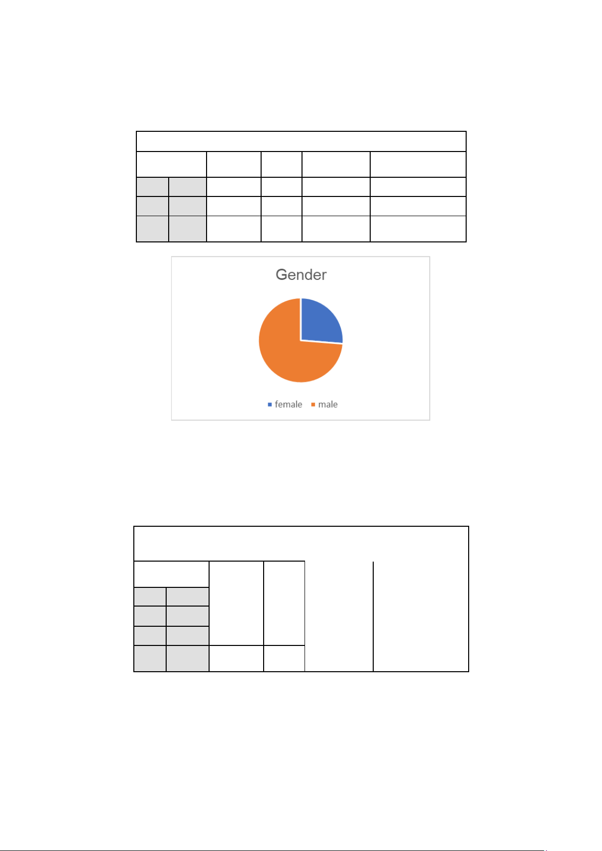
1. Descriptive statistics 1.1 Demographic 1.1.1 Gender Gender
Frequency Percent Valid Percent Cumulative Percent Valid female 280 26,3 26,3 26,3 male 785 73,7 73,7 100,0 Total 1065 100,0 100,0
Chart 1: Descriptive statistics on gender
According to the results, men make up the majority of approximately 74%, women about 26%. This
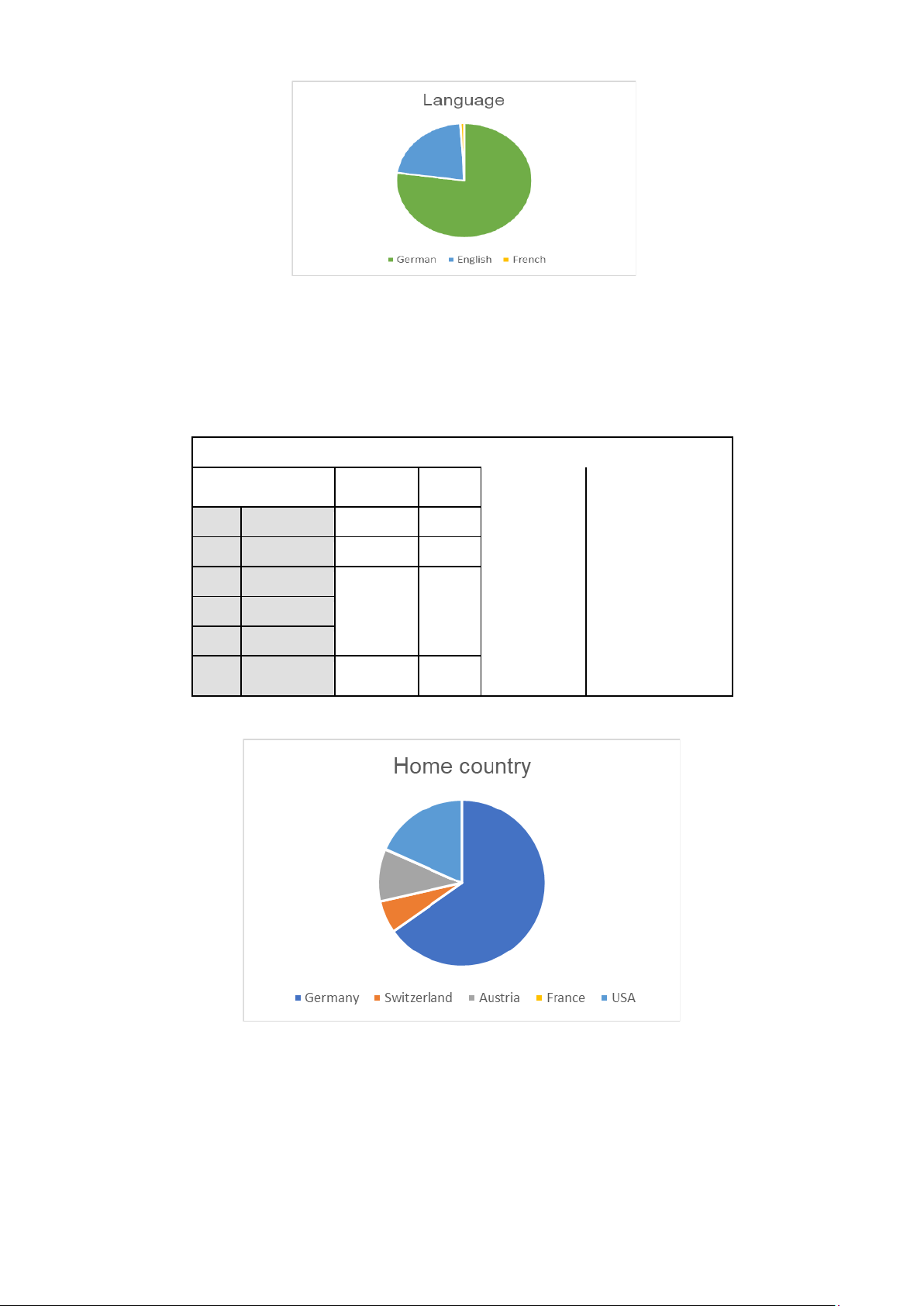
shows that the sample is full of 2 sexes 1.1.2 Language Language
Frequency Percent Valid Percent Cumulative Percent Valid German 822 77,2 77,2 77,2 English 233 21,9 21,9 99,1 French 10 ,9 ,9 100,0 Total 1065 100,0 100,0
Chart 2: Descriptive statistics on Language
According to the survey, respondents use 3 languages: German, English, French. In which, the most used
language is German, accounting for 77.2%, followed by English about 22%. 1.1.3 Home Country Home country
Frequency Percent Valid Percent Cumulative Percent Valid Germany 695 65,3 65,3 65,3 Switzerland 66 6,2 6,2 71,5 Austria 108 10,1 10,1 81,6 France 1 ,1 ,1 81,7 USA 195 18,3 18,3 100,0 Total 1065 100,0 100,0
Chart 3: Descriptive statistics on Home country
According to the survey, respondents came from many different countries: Germany, Switzerland,
Austria, France, USA. In which, Germany accounts for the highest about 65%, USA accounts for about 18%,...
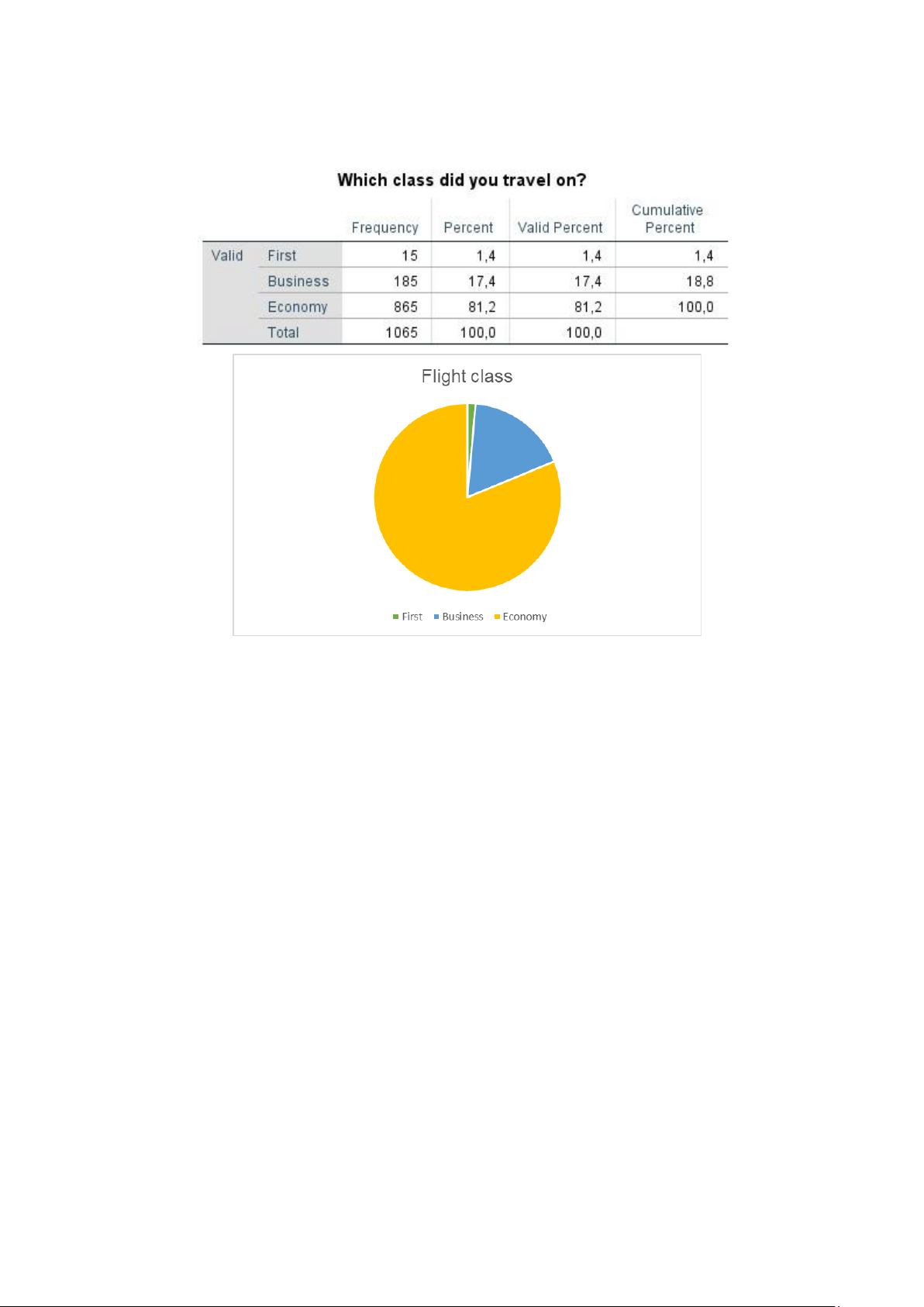
1.2 Flight Behavior measures 1.2.1 Flight class
Chart 4: Descriptive statistics on Fight-class
According to statistics, the most used flight class is economy accounting for about 81%, followed by
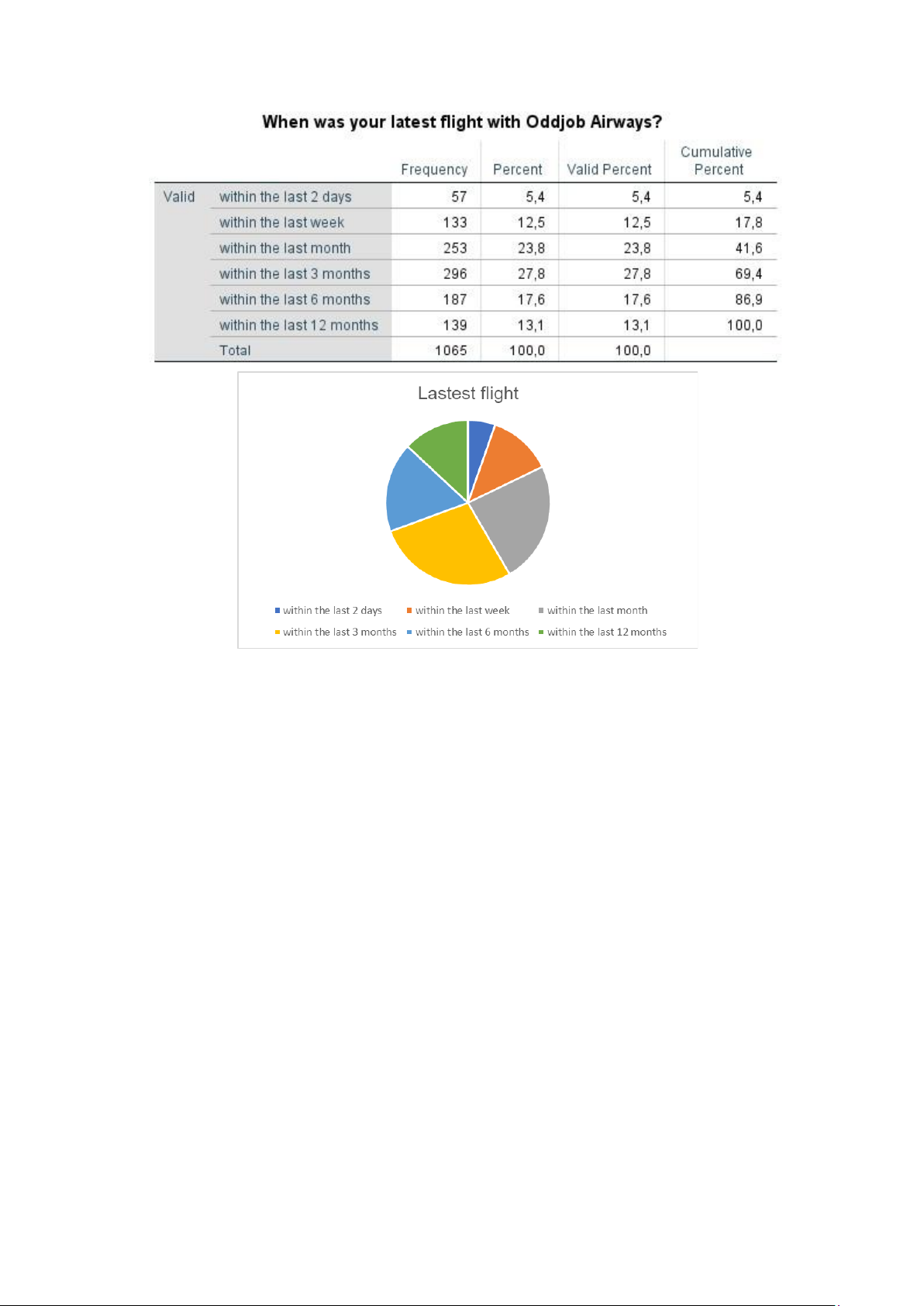
business accounting for more than 17%. 1.2.2 Latest flight
Chart 5: Descriptive statistics on Flight-lastest
The survey shows that the passenger's last flight with Oddjob airway was from the last 2 days to 12
months. Most of the passengers with the last flight in the last 3 months accounted for about 28%, the
passengers with the flight in the last 2 days accounted for the lowest proportion of 5.4%. 1.2.3 Flight purpose
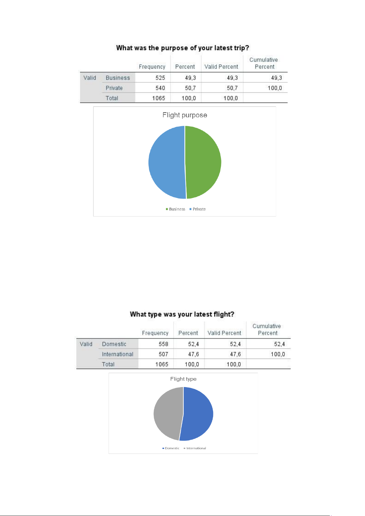
Chart 6; Descriptive statistics on Flight-purpose
The purpose of the flight is mainly: Private, Business. customers use for 2 similar purposes, but
private still has a slightly larger result. 1.2.4 Flight type
Chart 7: Descriptive statistics on Flight-type
The closest flight type used by customers is Domestic and International. In which, Domestic accounts
for a larger proportion of about 53%. 1.2.5 Number of flight
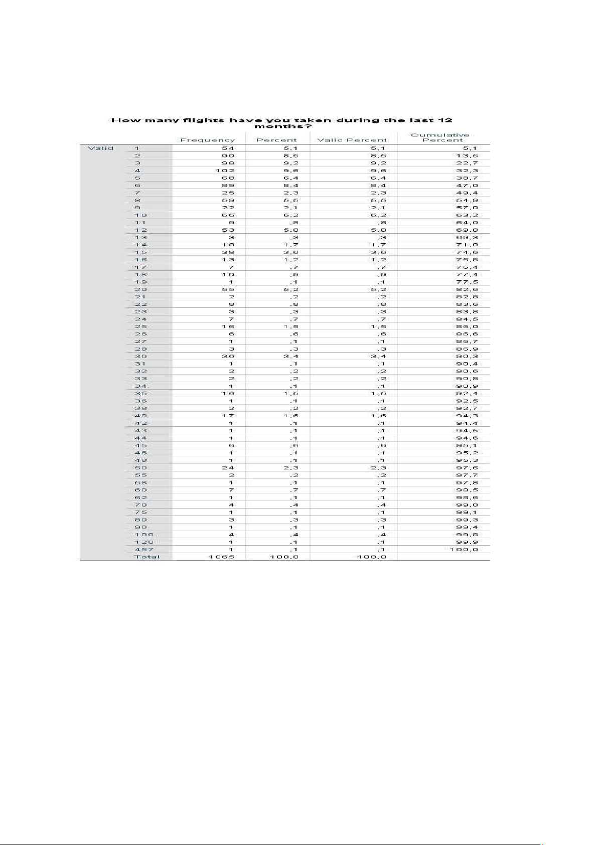
Table 1: Descriptive statistics on Flight-n
The above statistics show the number of passenger flights in 12 months. The question has many
answers from 1 to 457. customers mostly took less than 50 flights during the past 12 months, 457 flights is the least answer. 1.2.6 Traveler’s status
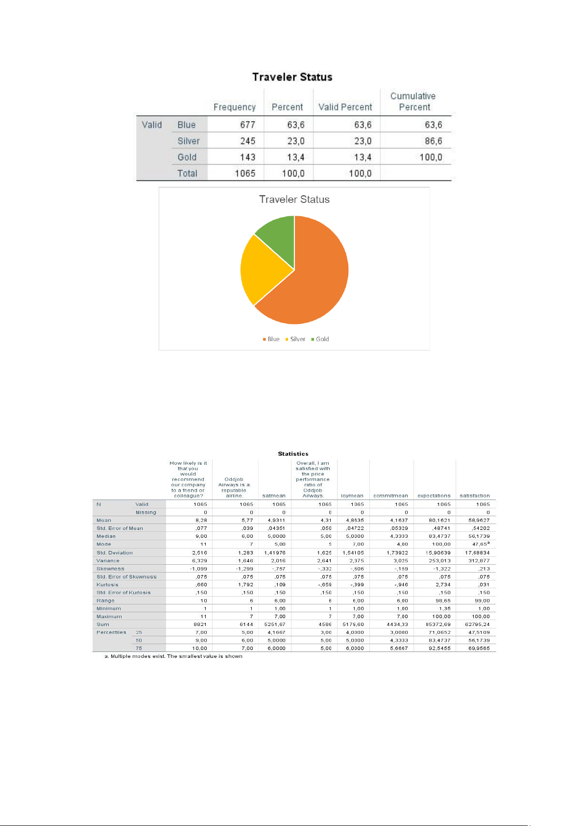
Chart 8: Descriptive statistics on Traveler’ Status
Membership status or membership class represents the customer's flight usage for Oddjob Airway. The
highest member class is Blue about 67%, the lowest is Gold 13%.
1.3 Perception and satisfaction measures
Table 2: Descriptive statistics on satisfaction
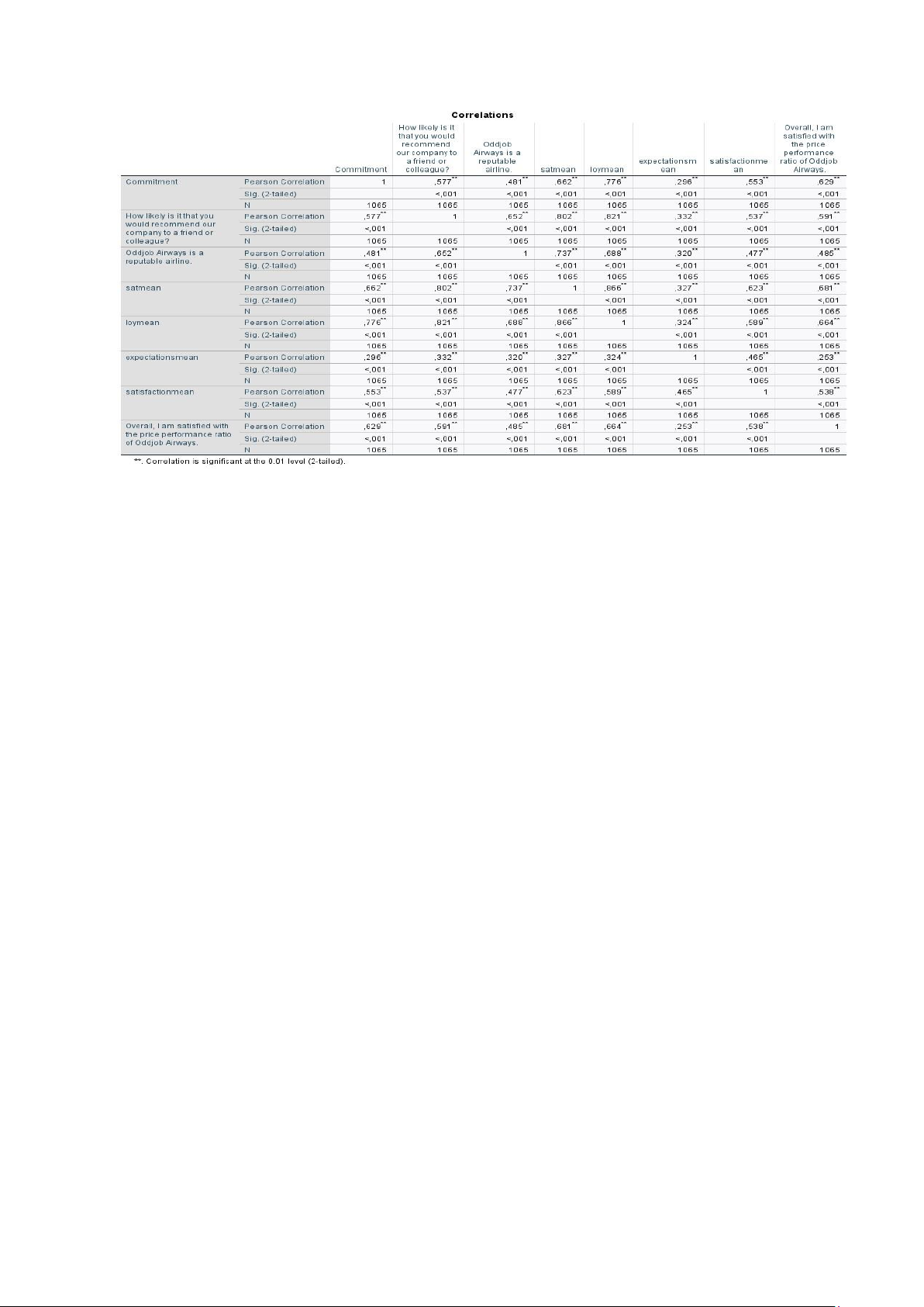
2. Pearson correlation analysis
Table 3: Measuring the correlation between variables
Dependent variable Note: When sig is less than 0.05, where the correlation coefficient Pearson we will see the symbol * or **.
The symbol ** indicates that this pair of variables has a linear correlation at the 99% confidence level
(corresponding to significance level 1% = 0.01).
2.1 Correlation between independent variable and dependent variable
With the above Pearson correlation results, the sig test of the correlation between the 7 independent
variables nps, reputation, satmean, overall-sat, loymean, expectations and satisfaction with the
dependent variable Commitment are all less than 0.05. Thus, there is a linear relationship between
these independent variables and the dependent variable.
2.2 Correlation between independent variables
Among the independent variables, there is no strong correlation when the absolute value of the
correlation coefficient between the pairs of variables is less than 0.5. Thus, the possibility of
collinearity/multicollinearity is also lower.
Run the regression analysis via spss with 1 dependent variable (commitmean) and 7 independent variables.
This table is used to evaluate the goodness of fit. We can see that Adjusted R square is 0.653 which
means 65.3% of the fluctuation of commitmean is explained by 7 independents. 34.7% left can be
explained by other independents and indeterminate errors.
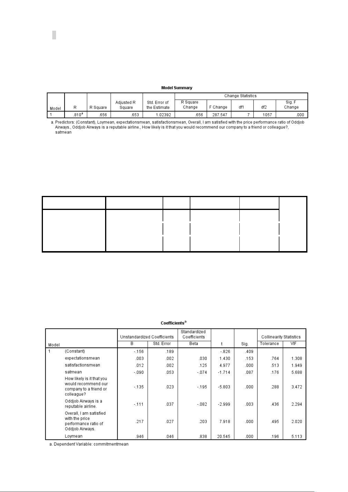
3. Linear regression analysis 3.1 First run 3.1.1 Linear regression
Run the regression analysis via spss with 1 dependent variable (commitmean) and 7 independent variables:
This table is used to evaluate the goodness of fit. We can see that Adjusted R square is 0.653 which
means 65.3% of the fluctuation of commitmean is explained by 7 independents. 34.7% left can be
explained by other independents and indeterminate errors. ANOVAa Model Sum of Squares df Mean Square F Sig. 1 Regression 2110.284 7 301.469 287.547 .000b Residual 1108.179 1057 1.048 Total 3218.463 1064
a. Dependent Variable: commitmean
b. Predictors: (Constant), Expectations, Overall, I am satisfied with the price performance ratio of
Oddjob Airways., Oddjob Airways is a reputable airline., Satisfaction, How likely is it that you
would recommend our company to a friend or colleague?, Loymean, Satmean
The ANOVA table gives us the result of the F test to evaluate the hypothesis of fit of the regression
model. F = 287.547 along with sig. = 0.000 < 5%, R square of the model is going to be different other
than 0 which means the regression model is suitable.
There are 2 variables that have sig. of t-test higher than 0.05 so these two might not explain much for
the fluctuation of the commitmean. Moreover, VIFs are also high so we consider removing two
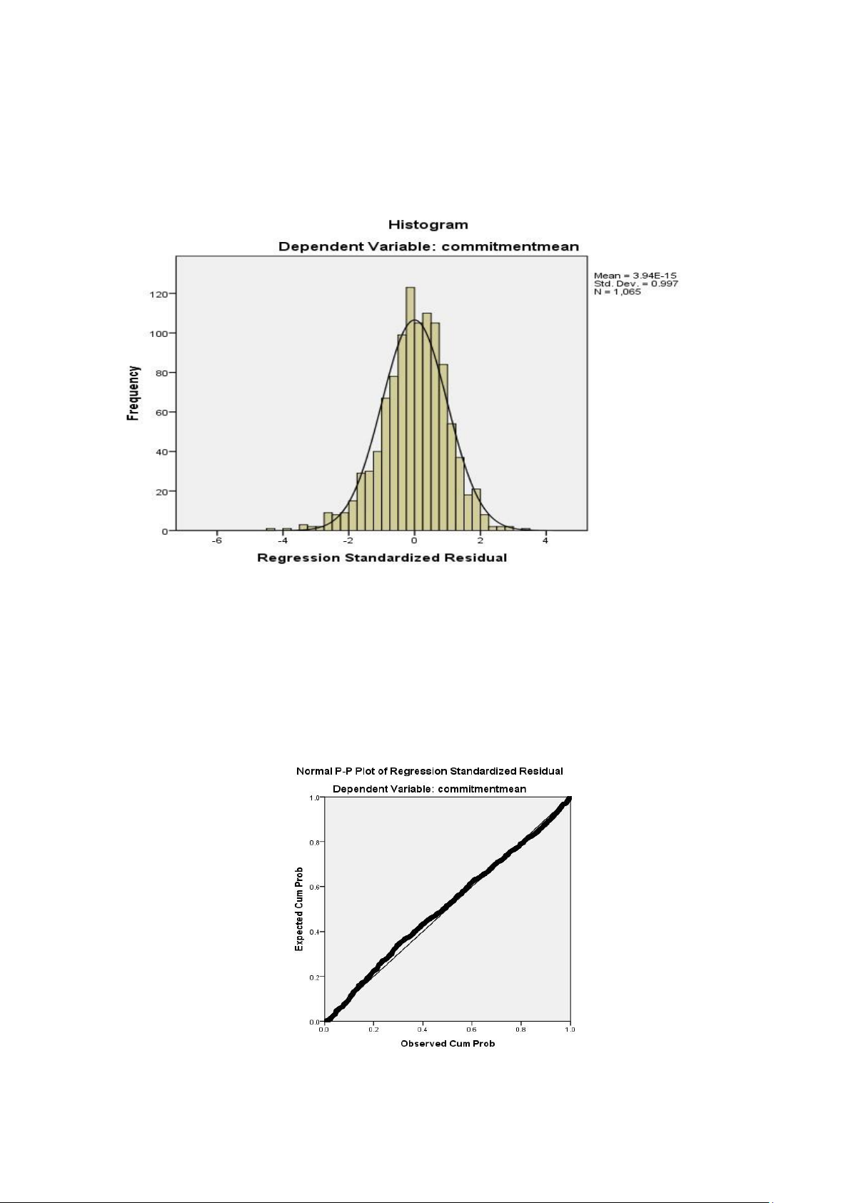
variables that have high sig. (expectations and satmean) 3.1.2 Histogram
Mean=3.94E-15= 3.4*10^-15 close to 0, standard deviation 0.997 close to 1. so to say , the residual
distribution is approximately normal, assuming the distribution The standard of residuals is not violated. 3.1.3 Normal P-P Plot
The residual data points are concentrated quite close to the diagonal, so that the residuals have an
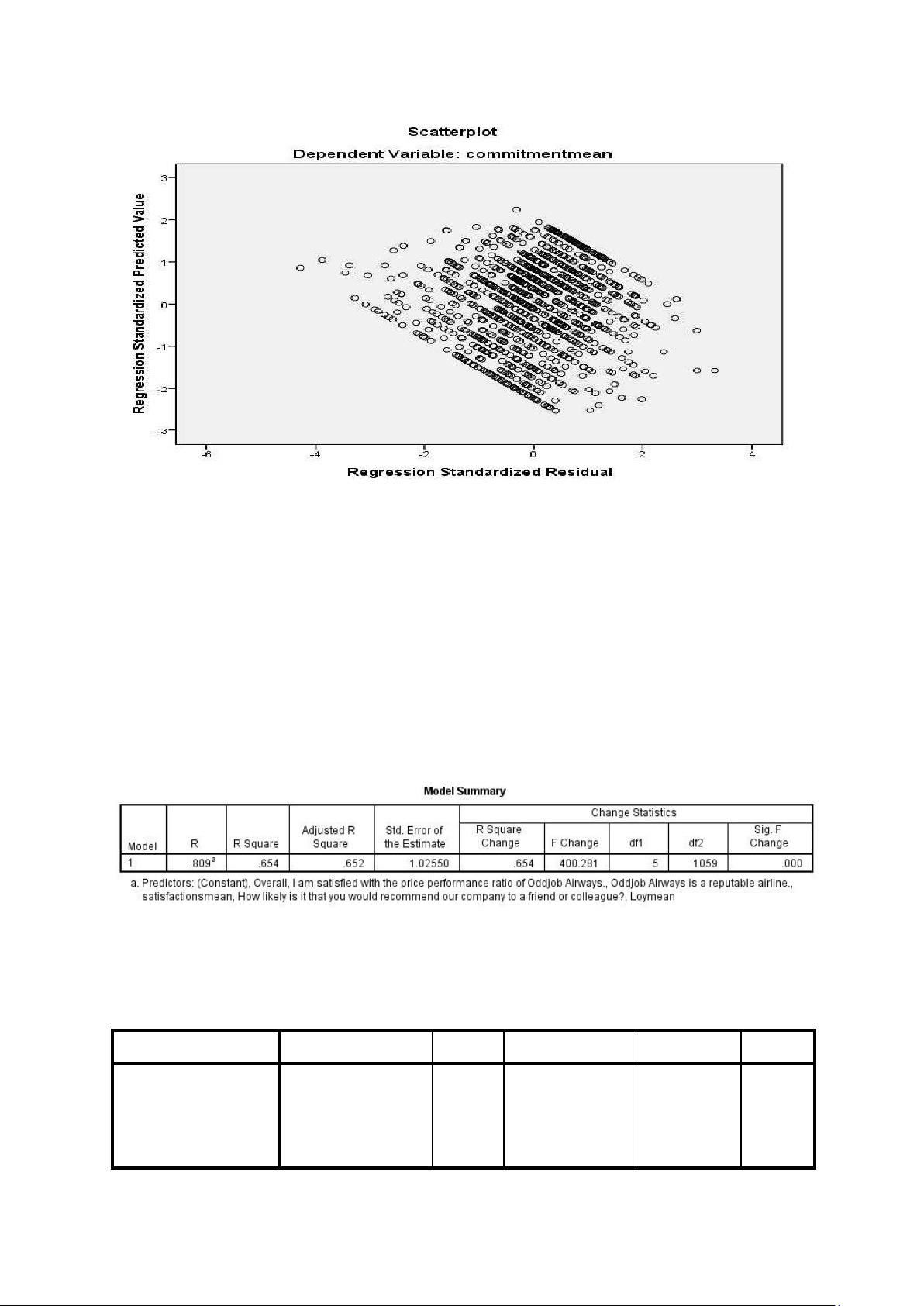
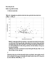
approximate normal distribution, assuming the normal distribution of the residuals is not violated 3.1.4 Scatter Plot
The normalized residuals are distributed centered around the zero line, so the assumption of a linear relationship is not violated. 3.2 Second run 3.2.1 Linear regression
After removing two variables, we run regression analysis again.
Adjusted R Square now is 65.2%, does not change much compared to 65.3% earlier, which means
commitmean fluctuation does not depend much on expectations and satmean. ANOVAa Model Sum of Squares df Mean Square F Sig. 1 Regression 2104.770 5 420.954 400.281 .000b Residual 1113.693 1059 1.052 Total 3218.463 1064
a. Dependent Variable: commitmentmean
b. Predictors: (Constant), Overall, I am satisfied with the price performance ratio of Oddjob Airways.,
Oddjob Airways is a reputable airline., satisfactionsmean, How likely is it that you would
recommend our company to a friend or colleague?, Loymean
F has raised to 400.281 with sig. = 0.000 < 5%, this regression model is still acceptable.
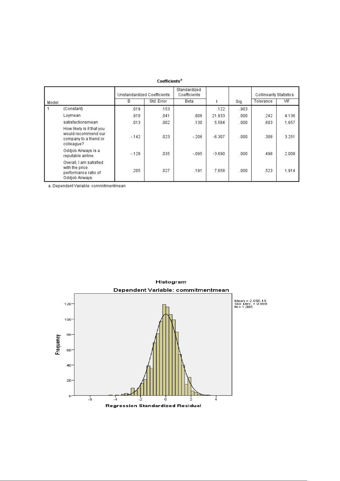
All of the sig. of t-tests are now lower than 5% which mean all of them have effect on commitmean
fluctuation. But considering VIF, there are two variables that are greatly higher than 2. Now that we
try to remove the 3rd variable since it has the minus t-test result and high VIF result. 3.2.2 Histogram
Mean=2.65E-15= 2.65*10^-15....close to 0, standard deviation 0.998 close to 1. So to say , the
residual distribution is approximately normal, assuming the distribution The standard of residuals is not violated. 3.2.3 Normal P-P Plot
The residual data points are concentrated quite close to the diagonal, so that the residuals have an
approximate normal distribution, assuming the normal distribution of the residuals is not violated 3.2.4 Scatter Plot
The normalized residuals are distributed centered around the zero line, so the assumption of a linear relationship is not violated. 3.3 Third run 3.3.1 Linear regression
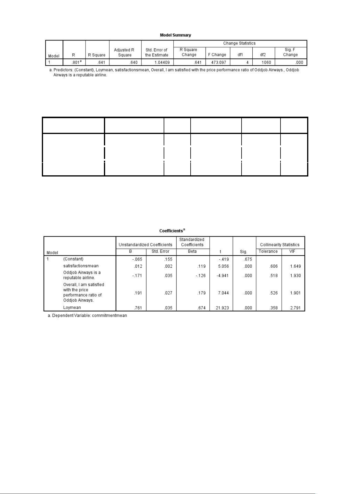
After removing, we run the regression analysis again with 4 independent variables left.
Adjusted R Square reduces to 64.0%, not much of a change to the Adjusted R Square of the model
above (65.2%), remaining acceptable. ANOVAa Model Sum of Squares df Mean Square F Sig. 1 Regression 2062.933 4 515.733 473.097 .000b Residual 1155.530 1060 1.090 Total 3218.463 1064
a. Dependent Variable: commitmentmean
b. Predictors: (Constant), Loymean, satisfactions, Overall, I am satisfied with the price performance
ratio of Oddjob Airways., Oddjob Airways is a reputable airline.
F has raised to 473.097 with sig. = 0.000 < 5%, this model is still acceptable.
All of the variables have the sig. = 0.000 < 5% which means all of them have statistical meanings to
dependent variables. Even though Loymean has the VIF higher than 2 but we tried to remove it from
the model, Adjust R Square reduces greatly to lower than 45% which might cause a great deal to the
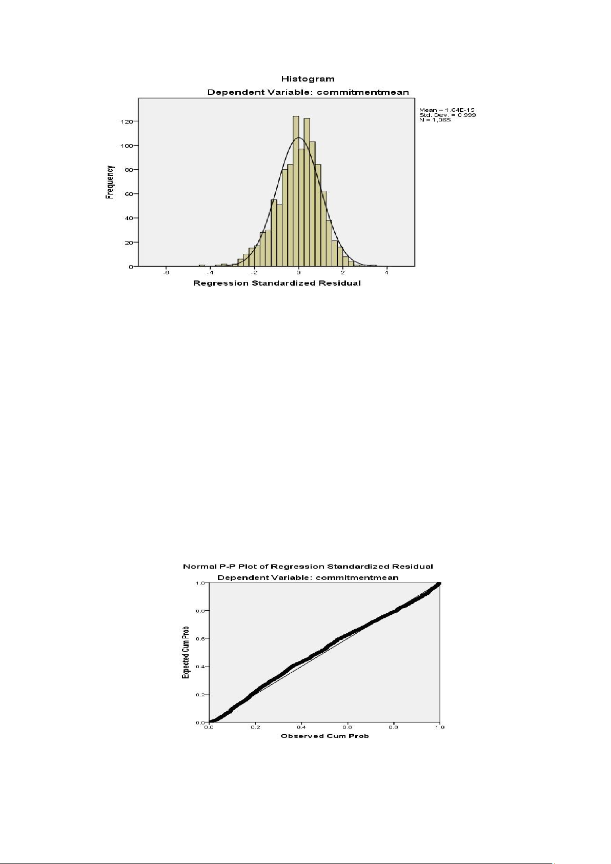
whole model so we accept the model with 4 independent variables. 3.3.2 Histogram
Mean=1.64E-15= 1.64*10^-15= 0.0000....close to 0, standard deviation 0.999 close to 1. so to say ,
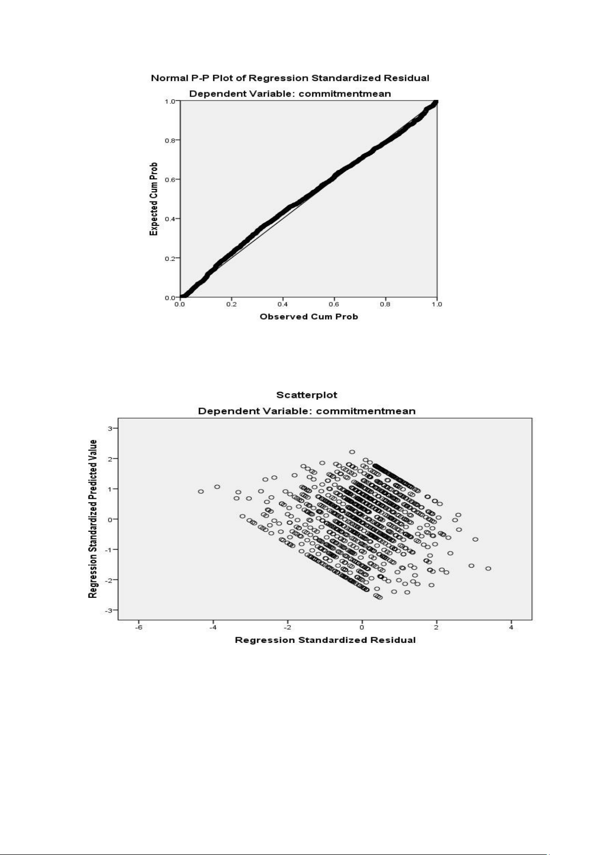
the residual distribution is approximately normal, assuming the distribution The standard of residuals is not violated. 3.3.3 Normal P-P Plot
The residual data points are concentrated quite close to the diagonal, so that the residuals have an
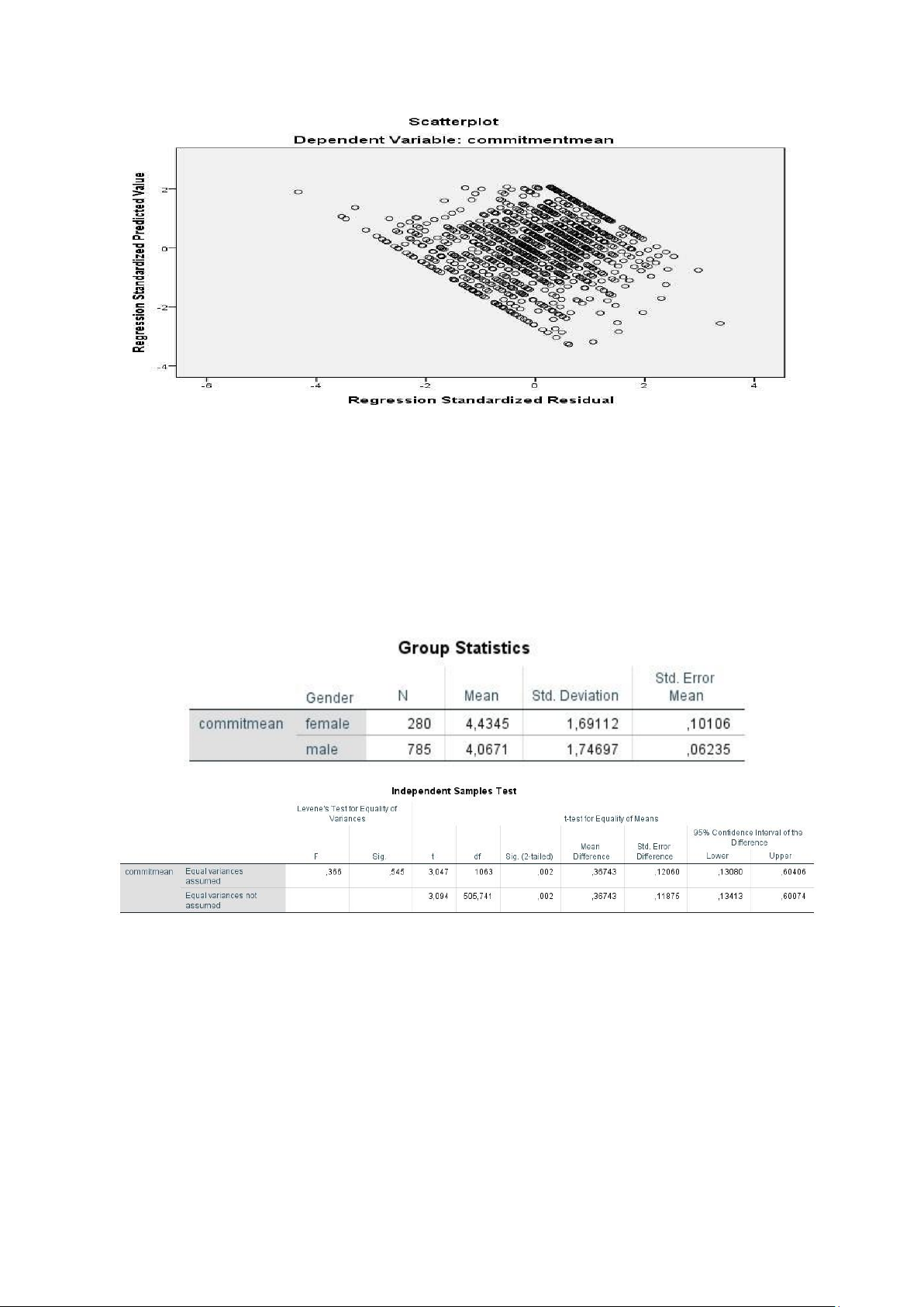
approximate normal distribution, assuming the normal distribution of the residuals is not violated. 3.3.4 Scatter Plot
The normalized residuals are distributed centered around the zero line and tend to form a straight line,
the linear relationship assumption is not violated, so the linear relationship assumption is not violated 3.4 T-test
Do sig in Levene's test = 0.545 >0.05
-> variance is not different
-> Using assumed Equal variances results We have
Sig(2-tailed) T-test = 0.02<0.05
Conclusion: There is a difference between male and female 4. Conclusion
Depending on the standardized coefficients Beta, in descending order of effecting on the dependent
variables, the highest one goes from Loymean, Overall_sat, satisfactionsmean and reputable airline,
which will be signed as loymean, overallsat, satmean and rep in the standardized regression equation below.
Commitmean = 0.674loymean + 0.179overallsat + 0.119satmean - 0.126rep + 𝜀
From the equation, we can say:
- 1 ascending unit of loymean cause 0.674 ascending unit of commitmean
- 1 ascending unit of overallsat cause 0.179 ascending unit of commitmean
- 1 ascending unit of satmean cause 0.119 ascending unit of commitmean - 1 ascending unit of rep
cause 0.126 descending unit of commitmean