Cal1 Final August 23 - Calculus 1 | Trường Đại học Quốc tế, Đại học Quốc gia Thành phố HCM
Cal1 Final August 23 - Calculus 1 | Trường Đại học Quốc tế, Đại học Quốc gia Thành phố HCM được sưu tầm và soạn thảo dưới dạng file PDF để gửi tới các bạn sinh viên cùng tham khảo, ôn tập đầy đủ kiến thức, chuẩn bị cho các buổi học thật tốt. Mời bạn đọc đón xem!
Môn: Calculus 1 (MA001IU) 44 tài liệu
Trường: Trường Đại học Quốc tế, Đại học Quốc gia Thành phố Hồ Chí Minh 2 K tài liệu
Tác giả:


Preview text:
Derivatives 2
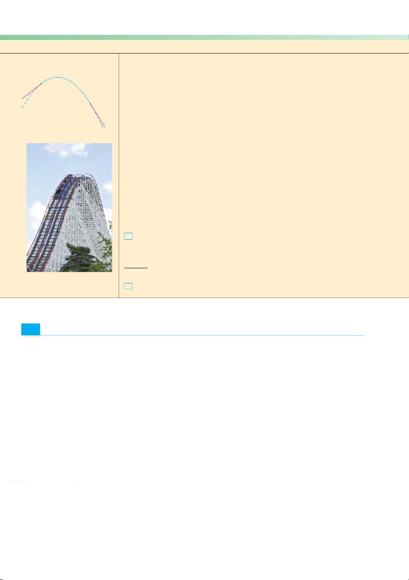
For a roller coaster ride to be smooth,
the straight stretches of the track need
to be connected to the curved segments
so that there are no abrupt changes in
direction. In the project on page 140
you will see how to design the first
ascent and drop of a new coaster for a smooth ride.
© Brett Mulcahy / Shutterstock
In this chapter we begin our study of differential calculus, which is concerned with how one quantity
changes in relation to another quantity. The central concept of differential calculus is the derivative,
which is an outgrowth of the velocities and slopes of tangents that we considered in Chapter 1. After
learning how to calculate derivatives, we use them to solve problems involving rates of change and the approximation of functions. 103 104 CHAPTER 2 2.1
Derivatives and Rates of Change
The problem of finding the tangent line to a curve and the problem of finding the velocity
of an object both involve finding the same type of limit, as we saw in Section 1.4. This spe-
cial type of limit is called a derivative and we will see that it can be interpreted as a rate of
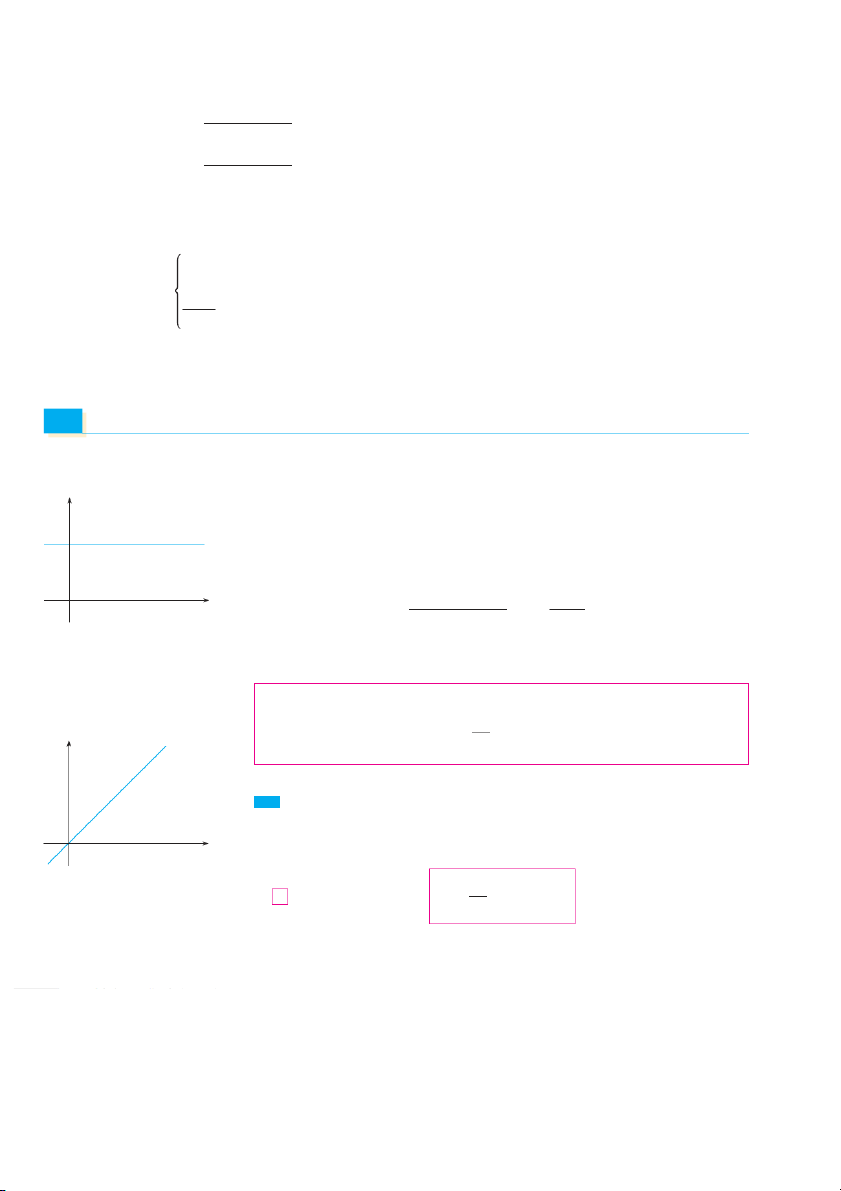
change in any of the sciences or engineering. Tangents y
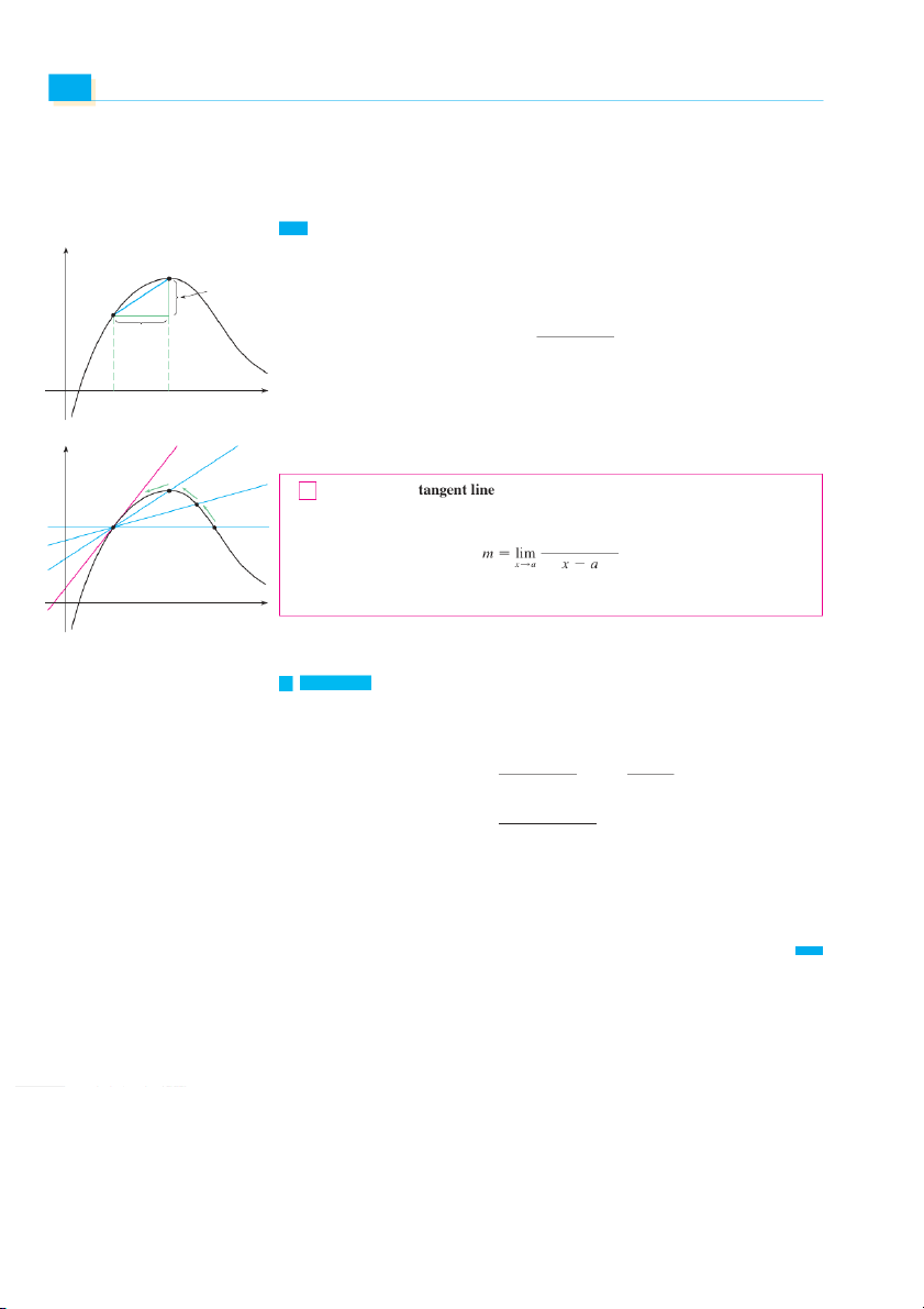
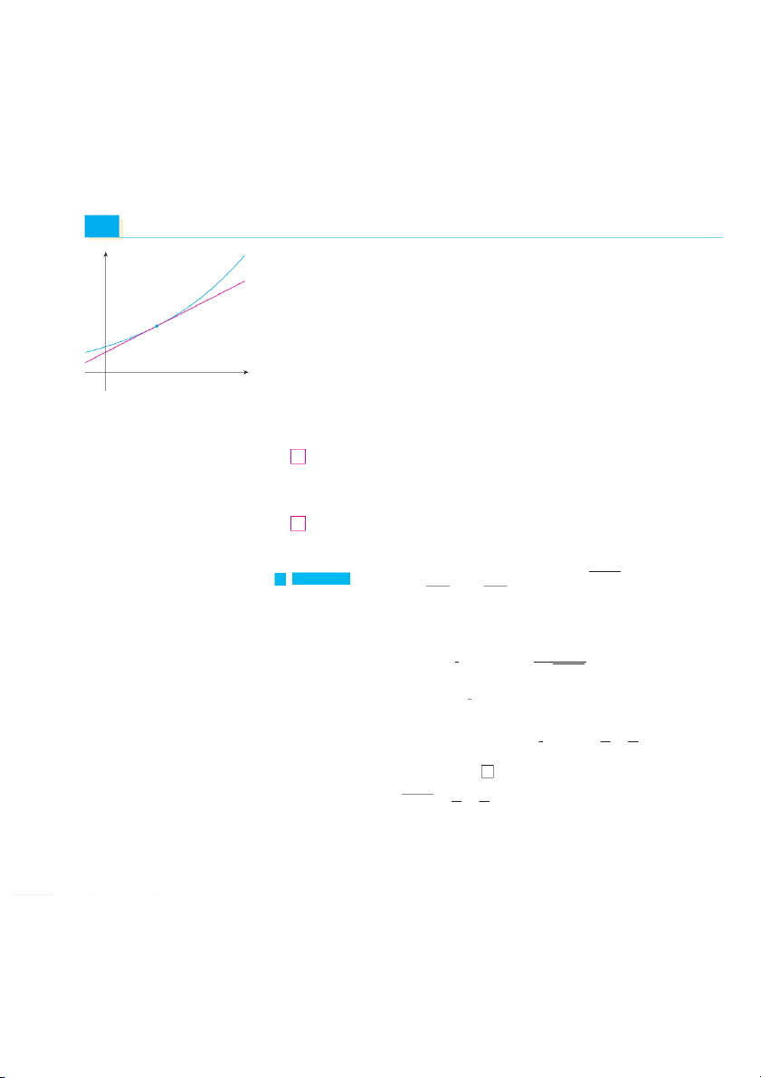
If a curve C has equation y 苷 f 共x兲 and we want to find the tangent line to C at the point Q{x,ƒ}
P共a, f 共a兲 ,
兲 then we consider a nearby point Q共x, f 共x兲 ,兲 where x 苷 ,
a and compute the slope ƒ-f(a) of the secant line PQ : P{a,f(a)}
f 共x兲 ⫺ f 共a兲 x-a m 苷 PQ x ⫺ a
Then we let Q approach P along the curve C by letting x approach a. If mPQ approaches a 0 a x
x number m, then we define the tangent t to be the line through P with slope m . (This
amounts to saying that the tangent line is the limiting position of the secant line PQ as Q
approaches P. See Figure 1.) y t Q Q 1 Definition The
to the curve y 苷 f 共x兲 at the point P共a, f 共a兲兲 is the
line through P with slope P Q
f 共x兲 ⫺ f 共a兲
provided that this limit exists. 0 x
In our first example we confirm the guess we made in Example 1 in Section 1.4. FIGURE 1 v
Find an equation of the tangent line to the parabola y 苷 x 2 EXAMPLE 1 at the point P共1, 1兲. SOLUTION Here we have
and f 共x兲 苷 x 2 a 苷 1 , so the slope is
f 共x兲 ⫺ f 共 兲 1 x 2 ⫺ 1 m 苷 lim 苷 lim x l1 x ⫺ 1 x l1 x ⫺ 1
共x ⫺ 1兲共x ⫹ 1兲 苷 lim x l1 x ⫺ 1
苷 lim 共x ⫹ 1兲 苷 苷 1 ⫹ 1 2 x l1
Point-slope form for a line through the
Using the point-slope form of the equation of a line, we find that an equation of the point 共x1 y , 1兲 with slope m: tangent line at 共1, 1兲 is y ⫺ y 苷 1
m共x ⫺ x1兲
y ⫺ 1 苷 2共x ⫺ 1兲 or y 苷 2x ⫺ 1
We sometimes refer to the slope of the tangent line to a curve at a point as the slope of
the curve at the point. The idea is that if we zoom in far enough toward the point, the curve
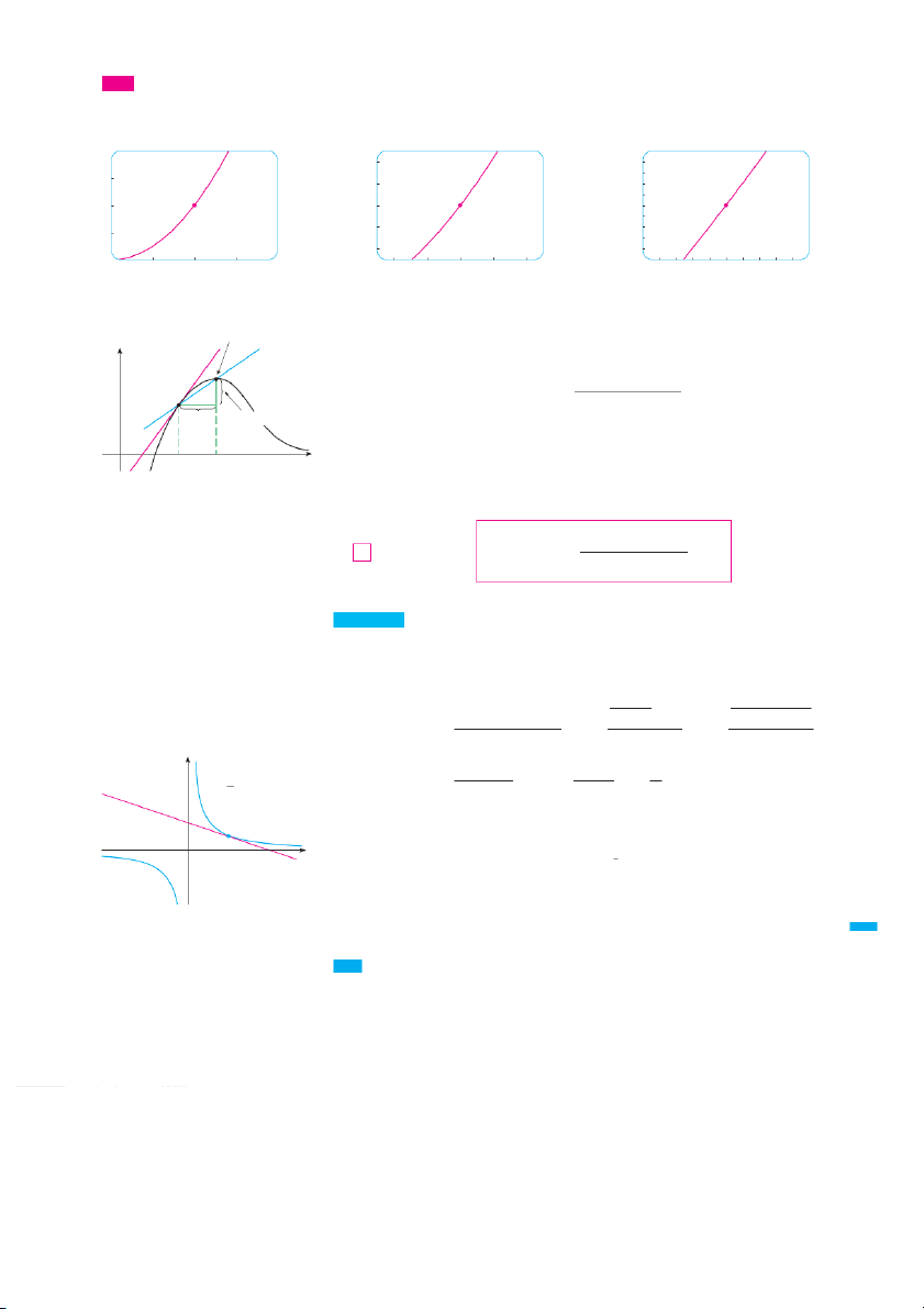
looks almost like a straight line. Figure 2 illustrates this procedure for the curve y 苷 x 2 in
D E R I VAT I V E S A N D R AT E S O F C H A N G E 105
TEC Visual 2.1 shows an animation of
Example 1. The more we zoom in, the more the parabola looks like a line. In other words, Figure 2.
the curve becomes almost indistinguishable from its tangent line. 2 1.5 1.1 (1,1) (1,1) (1,1) 0 2 0.5 1.5 0.9 1.1
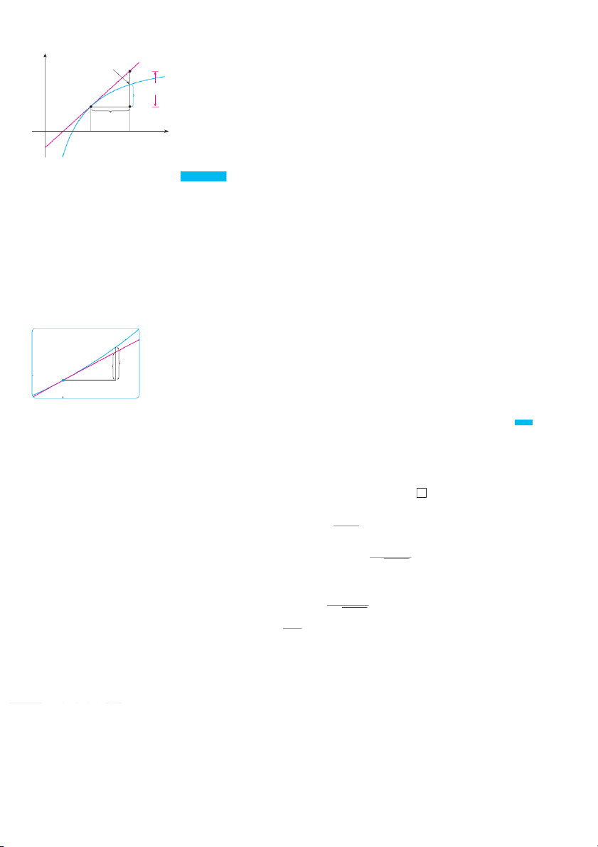
FIGURE 2 Zooming in toward the point (1,1) on the parabola y=≈ Q{a+h,f(a+h)}
There is another expression for the slope of a tangent line that is sometimes easier to y use. If h t
苷 x ⫺ a, then x 苷 a ⫹ h and so the slope of the secant line PQ is
f 共a ⫹ h兲 ⫺ f 共a兲 mPQ P{a,f(a)} 苷 h h f(a+h)-f(a)
(See Figure 3 where the case h ⬎ 0 is illustrated and Q is to the right of . P If it happened
that h ⬍ 0, however, Q would be to the left of . P ) 0 a a+h x
Notice that as x approaches ,
a h approaches 0 (because h 苷 x ⫺ ) a and so the expres- FIGURE 3
sion for the slope of the tangent line in Definition 1 becomes
f 共a ⫹ h兲 ⫺ f 共a兲 2 m 苷 lim h l 0 h EXAMPLE 2
Find an equation of the tangent line to the hyperbola y 苷 3兾x at the point 共3, 1兲.
SOLUTION Let f 共x兲 苷 3兾x. Then the slope of the tangent at 共 兲 3, 1 is 3 3 ⫺ 共3 ⫹ h兲 ⫺ 1
f 共3 ⫹ h兲 ⫺ f 共 兲 3 3 ⫹ h 3 ⫹ h m 苷 lim 苷 lim 苷 lim h l 0 h h l 0 h h l 0 h y ⫺h 1 1 x+3y-6=0 3 苷 lim 苷 lim ⫺ 苷 ⫺ y= h x
l 0 h共3 ⫹ h兲 h l 0 3 ⫹ h 3 (3,1)
Therefore an equation of the tangent at the point 共3, 1兲 is 0 x y 1 ⫺ 1 苷 ⫺ 共x 3 ⫺ 3兲 which simplifies to x ⫹ y 3 ⫺ 6 苷 0 FIGURE 4
The hyperbola and its tangent are shown in Figure 4. Velocities
In Section 1.4 we investigated the motion of a ball dropped from the CN Tower and defined
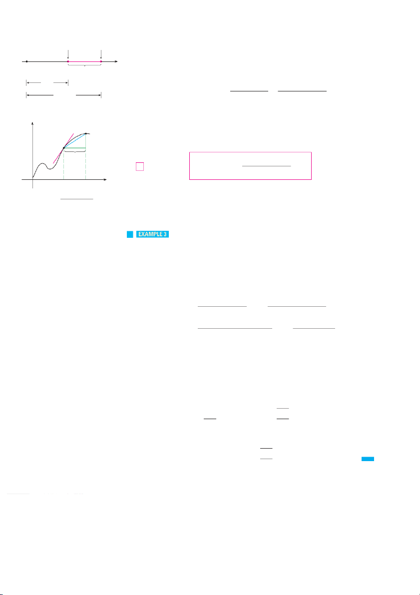
its velocity to be the limiting value of average velocities over shorter and shorter time periods. 106 CHAPTER 2 position at position at
In general, suppose an object moves along a straight line according to an equation of time t=a time t=a+h motion s 苷 f , 共 twh
兲 ere s is the displacement (directed distance) of the object from the ori-
gin at time t . The function f that describes the motion is called the position function
of the object. In the time interval from t 苷 a to t 苷 a ⫹ h the change in position is 0 s f(a+h)-f(a)
f 共a ⫹ h兲 ⫺ f . (S 共 e a e F
兲 igure 5.) The average velocity over this time interval is f(a)
共a ⫹ h兲 ⫺ 共a兲
average velocity 苷 displacement 苷 f f f(a+h) time h FIGURE 5
which is the same as the slope of the secant line PQ in Figure 6.
Now suppose we compute the average velocities over shorter and shorter time intervals s Q{a+h, f(a+h)}
关a, a ⫹ .h In
兴 other words, we let h approach 0. As in the example of the falling ball, we
define the velocity (or instantaneous velocity) v共aat 兲time t to 苷 b a e the limit of these P average velocities: {a, f(a)} h
f 共a ⫹ h兲 ⫺ f 共a兲 3 v共a兲 苷 lim h l 0 h 0 a a+h t
This means that the velocity at time t 苷 ais equal to the slope of the tangent line at P (com- f(a+h)-f(a) mPQ= h pare Equations 2 and 3). ⫽ average velocity
Now that we know how to compute limits, let’s reconsider the problem of the fall- ing ball. FIGURE 6 v
Suppose that a ball is dropped from the upper observation deck of the
CN Tower, 450 m above the ground.
(a) What is the velocity of the ball after 5 seconds?
(b) How fast is the ball traveling when it hits the ground?
Recall from Section 1.4: The dis tance
SOLUTION We will need to find the velocity both when t 苷 5 and when the ball hits the
(in meters) fallen after seconds is 4.9t .2 t
ground, so it’s efficient to start by finding the velocity at a general time t 苷 . a Using the
equation of motion s 苷 f 共t兲 苷 , w 4.9te2 have
f 共a ⫹ h兲 ⫺ f 共 兲 a 4.9共a ⫹ 兲 h 2 ⫺ 4.9a2 v共a兲 苷 lim 苷 lim h l 0 h h l 0 h 共 苷 4.9
a 2 ⫹ 2ah ⫹ h 2 ⫺ a 2 兲 4.9 2 共 ah ⫹ h2兲 lim 苷 lim h l 0 h h l 0 h 苷 lim4.9 2
共 a ⫹ h兲 苷 9.8a h l 0
(a) The velocity after 5 s is v共5兲 苷 共9.8兲 m 共5 兾 兲 s.苷 49
(b) Since the observation deck is 450 m above the ground, the ball will hit the ground at the time wh t e
1 n s共t 兲 苷 1 , tha 450 t is, 4.9t 2 苷 1 450 This gives t 2 苷 450 1 and t 苷 4.9 冑450⬇9.6 s 1 4.9
The velocity of the ball as it hits the ground is therefore 冑450
v共t 兲 苷 9.8t ⬇ 94 m s 兾 1 苷 1 9.84.9
DERIVATIVES AND RATES OF CHANGE 107 Derivatives
We have seen that the same type of limit arises in finding the slope of a tangent line (Equa-
tion 2) or the velocity of an object (Equation 3). In fact, limits of the form f 共a h兲 f 共a兲 lim h l 0 h
arise whenever we calculate a rate of change in any of the sciences or engineering, such
as a rate of reaction in chemistry or a marginal cost in economics. Since this type of limit
occurs so widely, it is given a special name and notation.
4 Definition The derivative of a function f at a number a , denoted by f , 共 i a s 兲 f is 共rea a d 兲 “ prime f of a .” if this limit exists.
If we write x 苷 a ,
h then we have h 苷 x a a nd a h pproaches i 0 f and only if x
approaches a. Therefore an equivalent way of stating the definition of the derivative, as we
saw in finding tangent lines, is f 共x兲 f 共a兲 5
f 共a兲 苷 lim x l a x a v
Find the derivative of the function f 共x兲 苷 x 2 8xat the 9 number . a
SOLUTION From Definition 4 we have f 共a h兲 f 共 兲 a
f 共a兲 苷 lim h l 0 h 苷 关共a h兲2 8 a 共 h兲 9兴 关a2 8a 9兴 lim h l 0 h 2 2 2 苷 a 2ah h 8a h 8 9 a 8a 9 lim h l 0 h 苷 2ah h 2 8h lim 苷 lim共2a h 8兲 h l 0 h h l 0 苷 2a 8
We defined the tangent line to the curve y at 苷 th f e p 共 o x in
兲 t P共a, f 共to a b 兲e th 兲 e line that
passes through P and has slope m given by Equation 1 or 2. Since, by Defini tion 4, this is
the same as the derivative f , 共 w a e c 兲 an now say the following. The tangent line to at y 苷 f i 共s 共 a t , x h f e 兲 l 共in a e 兲thr
兲 ough 共a, f 共w a ho 兲 se 兲 slope is equal to f , 共 th a e
兲 derivative of f at . a 108 CHAPTER 2 If we
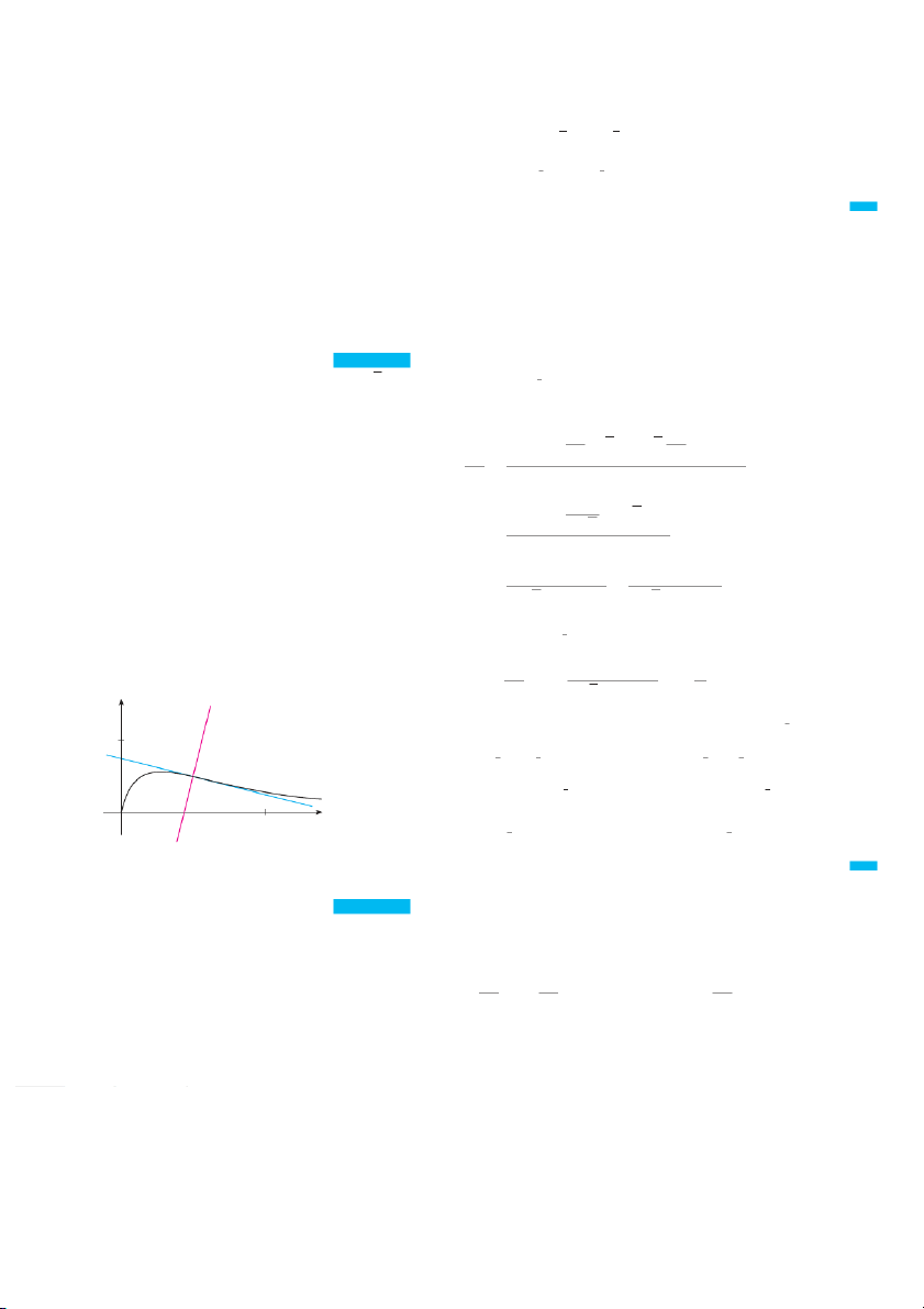
of the equation of a line, we can write an to the curve y at 苷 tfhe p 共xoin 兲 t 共a, f : 共a兲兲 y y=≈-8x+9 v Find an
of the tangent line to the parabola y 苷 x 2 8x at 9 0 x the point 共3, . 6兲
SOLUTION From Example 4 we know that the derivative of f共x兲 苷 x 2 8x at 9 the (3, _6)
number a is f 共a兲 苷 2a. The
8 refore the slope of the tangent line at 共 is 3, 6兲 y=_2x f 共3兲 苷 共 2 3兲 . T 8 hu 苷 s an
2 equation of the tangent line, shown in Figure 7, is FIGURE 7 y
共 6兲 苷 共 2兲共x or 3 兲 y 苷 2x Rates of Change
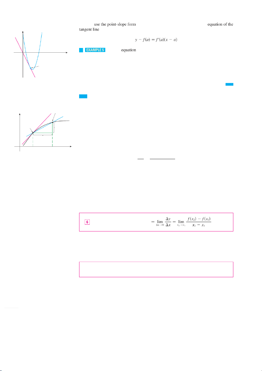
Suppose y is a quantity that depends on another quantity x. Thus y is a function of x and we
write y 苷 f 共. xIf
兲 chaxnges from 1 to xx2 , then the change in x (also called the increment Q{¤, ‡} y of ) x is x 苷 x2 x1 P{⁄, fl} Îy
and the corresponding change in y is Îx
y 苷 f 共x 兲 兲 2 f 共x1 0 ⁄ ¤ x The difference quotient y 共 兲 共 兲
average rate of change ⫽ mPQ 苷 f x2 f x1 x x2 x1
instantaneous rate of change ⫽ slope of tangent at P
is called the average rate of change of y with respect to x over the interval 关x 兴 1, x a 2 nd can FIGURE 8
be interpreted as the slope of the secant line PQ in Figure 8.
By analogy with velocity, we consider the average rate of change over smaller and
smaller intervals by letting x2 approach x1 and therefore letting x approach 0. The limit of
these average rates of change is called the (instantaneous) rate of change of y with respect to x at x ,
苷wxh1ich is interpreted as the slope of the tangent to the curve y 苷 f 共 a x t 兲 P共x 兲兲 1, f 共 : x1 instantaneous rate of change
We recognize this limit as being the derivative f 共 .x 兲 1
We know that one interpretation of the derivative f i 共sa as
兲 the slope of the tangent line
to the curve y 苷 f 共w x he 兲 n x 苷 .
a We now have a second interpretation: The derivative f is th 共 e a in
兲 stantaneous rate of change of y 苷 f 共 w x it 兲h respect
to x when x 苷 . a
DERIVATIVES AND RATES OF CHANGE 109 y
The connection with the first interpretation is that if we sketch the curve y 苷 f , x then
the instantaneous rate of change is the slope of the tangent to this curve at the point where Q x 苷 .
a This means that when the derivative is large (and therefore the curve is steep, as
at the point P in Figure 9), the -
y values change rapidly. When the derivative is small, the
curve is relatively flat (as at point Q ) and the y -values change slowly. P
In particular, if s 苷 f its the position function of a particle that moves along a straight line, then f i
a s the rate of change of the displacement wisth respect to the time . In t other words, f i
as the velocity of the particle at time t . T
苷 hae speed of the particle is
the absolute value of the velocity, that is, f a. x
In the next example we discuss the meaning of the derivative of a function that is defined verbally. FIGURE 9
The y-values are changing rapidly v
A manufacturer produces bolts of a fabric with a fixed width. The cost of
at P and slowly at Q.
producing x yards of this fabric is C 苷 f x dollars.
(a) What is the meaning of the derivative f ? x What are its units?
(b) In practical terms, what does it mean to say that f 1000 ? 苷 9
(c) Which do you think is greater, f o 50 r f ? Wh 500 at about f ? 5000 SOLUTION (a) The derivative f
ixs the instantaneous rate of change of C with respect to x; that is, f m
x eans the rate of change of the production cost with respect to the number of
yards produced. (Economists call this rate of change the marginal cost. This idea is dis-
cussed in more detail in Sections 2.7 and 3.7.) Because C f x 苷 lim x l 0 x the units for f a
x re the same as the units for the difference quotient C . Sin xce
Cis measured in dollars and i
x n yards, it follows that the units for f ar x e dollars per yard.
(b) The statement that f 1000 m
苷 e9ans that, after 1000 yards of fabric have been
manufactured, the rate at which the production cost is increasing is $9 yard. (When x 苷 ,
1000 C is increasing 9 times as fast as x.)
Here we are assuming that the cost function Since x 苷 i
1s small compared with x 苷 ,
1000 we could use the approximation
is well behaved; in other words, C x doesn’t
oscillate rapidly near x 苷 . 1000 C f 1000 苷 C 苷 C x 1
and say that the cost of manufacturing the 1000th yard (or the 1001st) is about $9.
(c) The rate at which the production cost is increasing (per yard) is probably lower
when x 苷 500 than when x 苷 50 (the cost of making the 500th yard is less than the cost
of the 50th yard) because of economies of scale. (The manufacturer makes more efficient
use of the fixed costs of production.) So f 50 f 500
But, as production expands, the resulting large-scale operation might become inefficient
and there might be overtime costs. Thus it is possible that the rate of increase of costs
will eventually start to rise. So it may happen that f 5000 f 500 110 CHAPTER 2
In the following example we estimate the rate of change of the national debt with respect
to time. Here the function is defined not by a formula but by a table of values. v
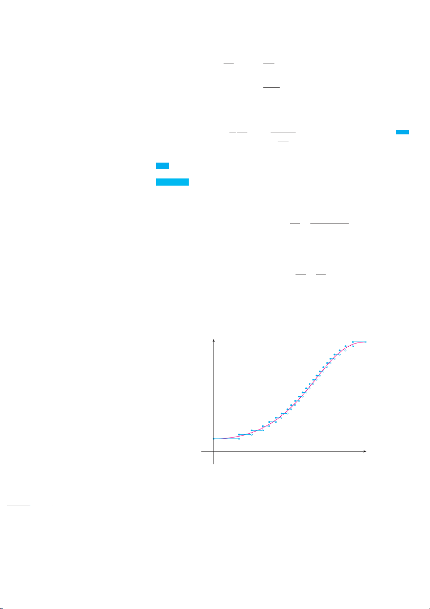
Let D t be the US national debt at time t. The table in the margin gives t D t
approximate values of this function by providing end of year estimates, in billions of dol- 1980 930.2
lars, from 1980 to 2005. Interpret and estimate the value of D . 1990 1985 1945.9
SOLUTION The derivative D
1990 means the rate of change of D with respect to t when 1990 3233.3 t 苷 ,
1990 that is, the rate of increase of the national debt in 1990. 1995 4974.0 According to Equation 5, 2000 5674.2 2005 7932.7 D t D 1990 D 1990 苷 lim t l1990 t 1990
So we compute and tabulate values of the difference quotient (the average rates of D t D 1990 t
change) as shown in the table at the left. From this table we see that D l 1990ies some- t 1990
where between 257.48 and 348.14 billion dollars per year. [Here we are making the 1980 230.31
reasonable assumption that the debt didn’t fluctuate wildly between 1980 and 2000.] We 1985 257.48
estimate that the rate of increase of the national debt of the United States in 1990 was 1995 348.14
the average of these two numbers, namely 2000 244.09 D 1990 303 billion dollars per year 2005 313.29
Another method would be to plot the debt function and estimate the slope of the tan- gent line when t 苷 . 1990 A Note on Units
The units for the average rate of change D t
In Examples 3, 6, and 7 we saw three specific examples of rates of change: the veloc-
are the units for D divided by the units for t
,ity of an object is the rate of change of displacement with respect to time; marginal cost is
namely, billions of dollars per year. The instan-
taneous rate of change is the limit of the aver- the rate of change of production cost with respect to the number of items produced; the
age rates of change, so it is measured in the
rate of change of the debt with respect to time is of interest in economics. Here is a small
same units: billions of dollars per year.
sample of other rates of change: In physics, the rate of change of work with respect to time
is called power. Chemists who study a chemical reaction are interested in the rate of
change in the concentration of a reactant with respect to time (called the rate of reaction).
A biologist is interested in the rate of change of the population of a colony of bacteria with
respect to time. In fact, the computation of rates of change is important in all of the natu-
ral sciences, in engineering, and even in the social sciences. Further examples will be given in Section 2.7.
All these rates of change are derivatives and can therefore be interpreted as slopes of
tangents. This gives added significance to the solution of the tangent problem. Whenever
we solve a problem involving tangent lines, we are not just solving a problem in geome-
try. We are also implicitly solving a great variety of problems involving rates of change in science and engineering. 2.1 Exercises
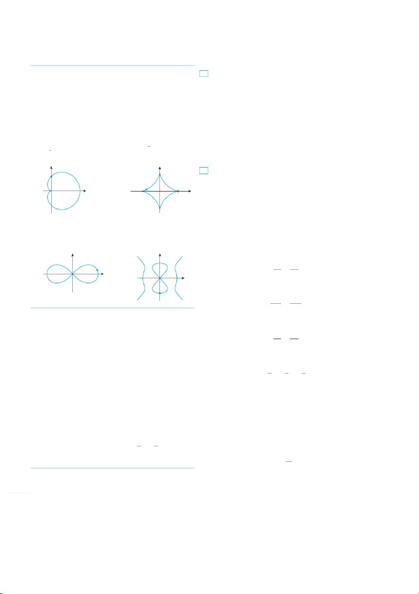
1. A curve has equation y 苷 f .x .
0.5, 0.5 What do you notice about the curve as you zoom
(a) Write an expression for the slope of the secant line in toward the origin?
through the points P 3, f 3and Q x . , f x
3. (a) Find the slope of the tangent line to the parabola
(b) Write an expression for the slope of the tangent line at P. y 苷 4x a xt 2 the point 1, 3 ; 2. Graph the curve in the viewing rectangles y 苷 sin x 2, 2 ( i) using Definition 1 ( ii) using Equation 2 by , 2, 2 by 1, 1 , and 1, 1 by 0.5, 0.5
(b) Find an equation of the tangent line in part (a).
; Graphing calculator or computer required
1. Homework Hints available at stewartcalculus.com
DERIVATIVES AND RATES OF CHANGE 111 ;
(b) At what time is the distance between the runners the
(c) Graph the parabola and the tangent line. As a check on greatest?
your work, zoom in toward the point 共 un 兲 1, 3 til the
(c) At what time do they have the same velocity?
parabola and the tangent line are indistinguishable.
4. (a) Find the slope of the tangent line to the curve y 苷 x x 3
13. If a ball is thrown into the air with a velocity of 40 ft兾s, its at the point 共 兲 1, 0
height ( in feet) after t seconds is given by y 苷 40t 16t .2 ( i) using Definition 1 ( ii) using Equation 2
Find the velocity when t 苷 .2
(b) Find an equation of the tangent line in part (a). ;
(c) Graph the curve and the tangent line in successively
14. If a rock is thrown upward on the planet Mars with a velocity
smaller viewing rectangles centered at 共 unt 兲 1, 0 il the of 10 m ,
兾 ists height ( in meters) after steconds is given by
curve and the line appear to coincide. H 苷 10t 1.86t .2
5–8 Find an equation of the tangent line to the curve at the
(a) Find the velocity of the rock after one second. given point.
(b) Find the velocity of the rock when t 苷 .a 5.
(c) When will the rock hit the surface? y 苷 4 , x 3x 共 2 2, 4 6. 兲 y 苷 x 3 3x, 共 1 兲 2, 3
(d) With what velocity will the rock hit the surface? 7.
y 苷 sx , (1, 1兲 8. y 苷 2x 1, 共 兲 1, 1 x 2
15. The displacement ( in meters) of a particle moving in a
straight line is given by the equation of motion s 苷 1 , 兾t2
9. (a) Find the slope of the tangent to the curve
where t is measured in seconds. Find the velocity of the par - 苷 苷 y 苷 3 4x 2
2x 3 at the point where x 苷 . a ticle at times t a t , 苷 t 1, 苷 , a 2 nd t .3
(b) Find equations of the tangent lines at the points 共 兲 1, 5 and 共 .兲 2, 3
16. The displacement ( in meters) of a particle moving in a ;
(c) Graph the curve and both tangents on a common screen.
straight line is given by s 苷 t 2 8t , 18 where tis mea- sured in seconds.
10. (a) Find the slope of the tangent to the curve y 苷 1兾sxat
(a) Find the average velocity over each time interval: the point where x 苷 . a ( i) 关3, 4兴 ( ii) 关3.5, 4兴
(b) Find equations of the tangent lines at the points 共 兲 1, 1 ( iii) 关4, 5兴 ( iv) 关4, 4.5兴 and (4, 1) 2 .
(b) Find the instantaneous velocity when t 苷 .4 ;
(c) Graph the curve and both tangents on a common screen.
(c) Draw the graph of sas a function of tand draw the secant
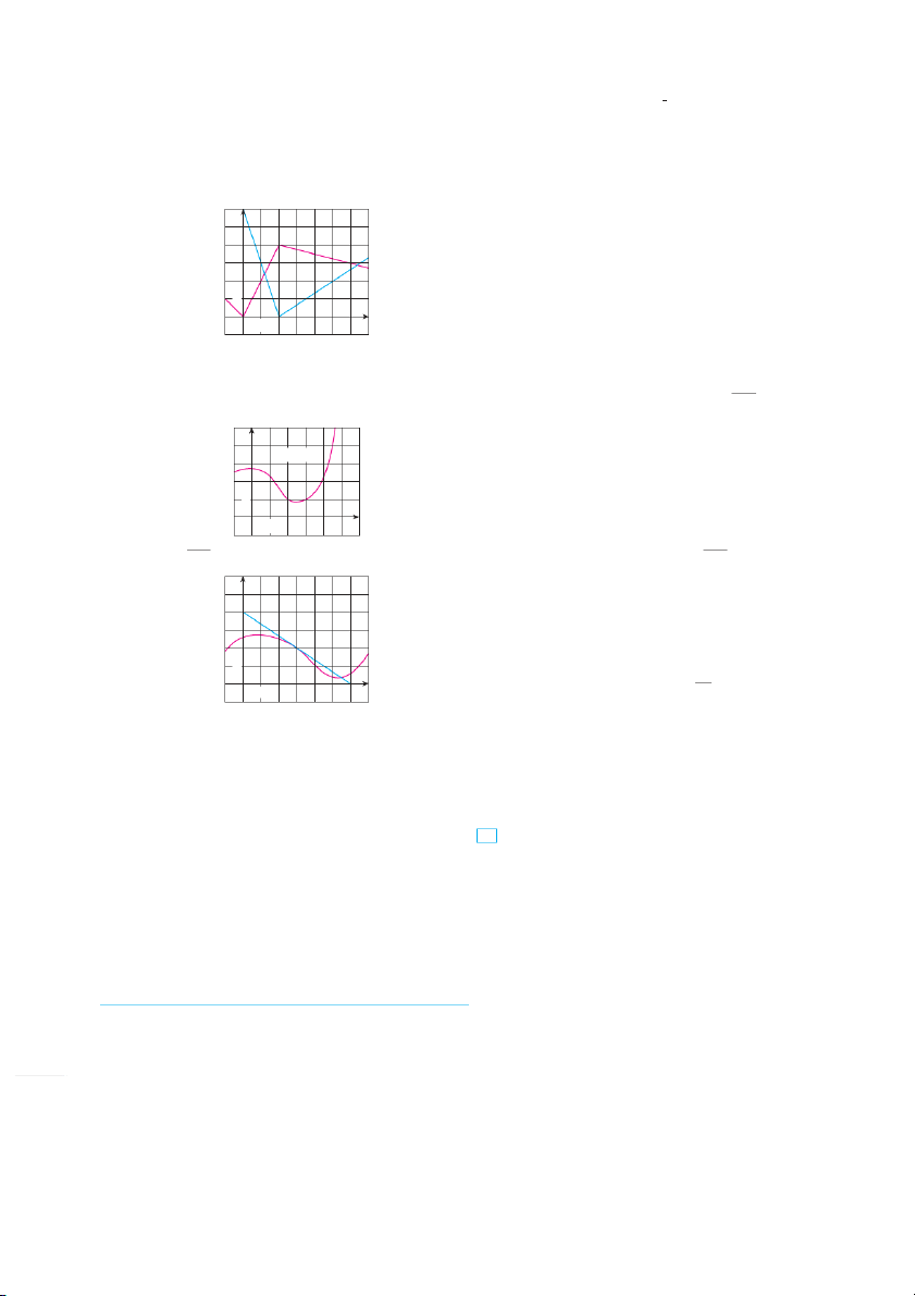
11. (a) A particle starts by moving to the right along a horizontal
lines whose slopes are the average velocities in part (a)
line; the graph of its position function is shown. When is
and the tangent line whose slope is the instantaneous
the particle moving to the right? Moving to the left? velocity in part (b). Standing still?
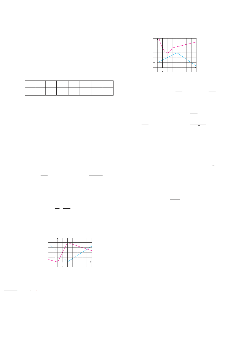
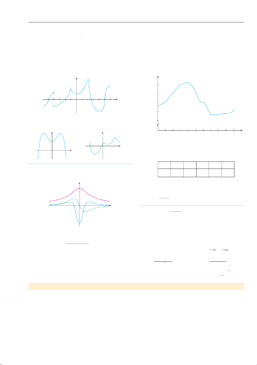
17. For the function t whose graph is given, arrange the follow-
(b) Draw a graph of the velocity function.
ing numbers in increasing order and explain your reasoning: s (meters) 4 0 t 共 2兲 t 共0兲 t 共2兲 t 共 兲 4 2 y y=© 0 2 4 6 t (seconds)
12. Shown are graphs of the position functions of two runners, A _1 0 1 3 4 x 2 and ,
B who run a 100-m race and finish in a tie. s (meters) 80
18. Find an equation of the tangent line to the graph of y 苷 t共x兲 A at x 苷 i 5 f t共5兲 苷 and 3 t 共 .5兲 苷 4 40 B
19. If an equation of the tangent line to the curve y 苷 f 共axt th 兲 e point where a 苷 i 2 s y 苷 4x , 5find f 共an 2 d 兲 .f 共 兲 2 0 4 8 12 t (seconds)
20. If the tangent line to y 苷 f 共axt (4 兲 , 3) passes through the
(a) Describe and compare how the runners run the race.
point (0, 2), find f 共 a 4 nd 兲 f . 共4兲 112 CHAPTER 2
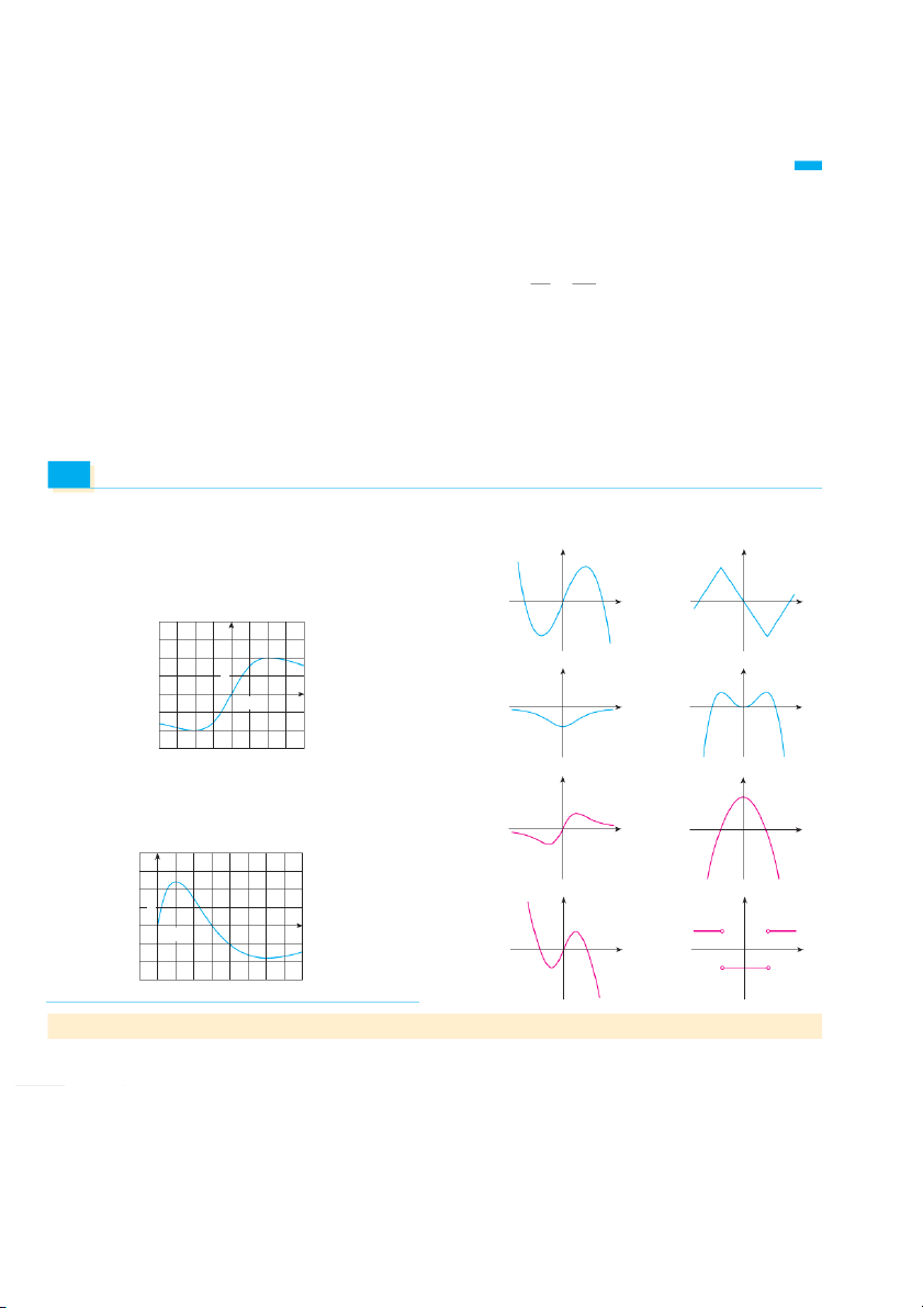
21. Sketch the graph of a function forf which f 共0兲 , 苷 0
the turkey decreases and eventually approaches room tempera- f ⬘共 f 0 ⬘ 兲 , 共a1 苷 nd 兲 3, f ⬘ 苷 共 0 2兲 . 苷 ⫺1
ture. By measuring the slope of the tangent, estimate the rate
of change of the temperature after an hour.
22. Sketch the graph of a function t for which t共0兲 苷 t共 ,2 t⬘ 兲 共 苷1兲 t共 苷 4 t 兲 ⬘ 苷 , 共0 3兲 t⬘ 苷 共0 0 兲 苷 t⬘ , 共4兲 苷 1 T (°F) t⬘共2兲 , lim 苷 ⫺1 ⬁ ⬁
x l 5⫺ t 共x兲 苷 , and limx l⫺1⫹ t共x兲 苷 ⫺. 200 23. If f 共x兲 苷 , 3 f x i 2 nd ⫺ f ⬘ x 3 共a 1nd
兲 use it to find an equation of the tangent line to the curve
y 苷 3x 2 ⫺atx t3he point 共 .兲 1, 2 P 24. If
t共x兲 苷 , xfi4nd ⫺ t⬘ 2 共 and 兲 1 use it to find an equation of 100 the tangent line to the curve y 苷 x 4 a
⫺ t 2the point 共1, ⫺ .兲 1 25. (a) If
F共x兲 苷 5x , 兾 fin 共 d 1 F ⫹ ⬘ x 共 2 a 兲 nd 兲 2 use it to find an
equation of the tangent line to the curve y 苷 5x兾共1 ⫹ x 2兲 0 30 60 90 120 150 t (min) at the point 共 .兲 2, 2 ;
(b) Illustrate part (a) by graphing the curve and the tangent
43. The number N of US cellular phone subscribers ( in millions) line on the same screen.
is shown in the table. (Midyear estimates are given.) 26. (a) If
G共x兲 苷 4, xfi 2 nd ⫺ G x ⬘ 3 共 and 兲 a use it to find equations
of the tangent lines to the curve y 苷 4x 2 ⫺ x 3 at the t 1996 1998 2000 2002 2004 2006 points 共 and 2, 8 共 兲 .兲 3, 9 N 44 69 109 141 182 233 ;
(b) Illustrate part (a) by graphing the curve and the tangent lines on the same screen.
(a) Find the average rate of cell phone growth ( i) from 2002 to 2006 ( ii) from 2002 to 2004
27–32 Find f ⬘共. 兲 a ( iii) from 2000 to 2002
In each case, include the units. 27.
f 共x兲 苷 3x 2 ⫺ 4x ⫹ 1
28. f 共t兲 苷 2t3 ⫹ t
(b) Estimate the instantaneous rate of growth in 2002 by
taking the average of two average rates of change. What 29.
30. f 共x兲 苷 x⫺2 f 共t兲 苷 2t ⫹ 1 t ⫹ 3 are its units?
(c) Estimate the instantaneous rate of growth in 2002 by mea-
31. f 共x兲 苷 s1 ⫺ 2x
32. f 共x兲 苷 4 suring the slope of a tangent. s1 ⫺ x
44. The number N of locations of a popular coffeehouse chain is
given in the table. (The numbers of locations as of October 1
33–38 Each limit represents the derivative of some function f at are given.) some number .
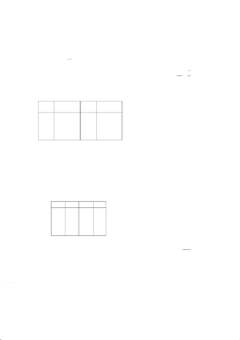
a State such an f and a in each case. 共1 ⫹ 兲 h 10 ⫺ 1 s4 16 ⫹ h ⫺ 2 Year 2004 2005 2006 2007 2008 33. lim 34. lim h l 0 h l 0 h h N 8569 10,241 12,440 15,011 16,680 2x ⫺ 32 tan x ⫺ 1 35. lim 36. lim
(a) Find the average rate of growth x l 5 x ⫺ 5 x l 兾4 x ⫺ 兾4 ( i) from 2006 to 2008 ( ii) from 2006 to 2007 ( iii) from 2005 to 2006 cos共 ⫹ h兲 ⫹ 1 t 4 ⫹ t ⫺ 2 37. lim 38. lim
In each case, include the units. h l 0 t l 1 h t ⫺ 1
(b) Estimate the instantaneous rate of growth in 2006 by
taking the average of two average rates of change. What
39 – 40 A particle moves along a straight line with equation of are its units? motion
(c) Estimate the instantaneous rate of growth in 2006 by mea- s 苷 f , 共 twh
兲 ere s is measured in meters and t in seconds.
Find the velocity and the speed when suring the slope of a tangent. t 苷 . 5
(d) Estimate the intantaneous rate of growth in 2007 and com-
39. f 共t兲 苷 100 ⫹ 50t ⫺ 4.9t2 40.
f 共t兲 苷 t ⫺1 ⫺ t
pare it with the growth rate in 2006. What do you conclude?
45. The cost ( in dollars) of producing x units of a certain com-
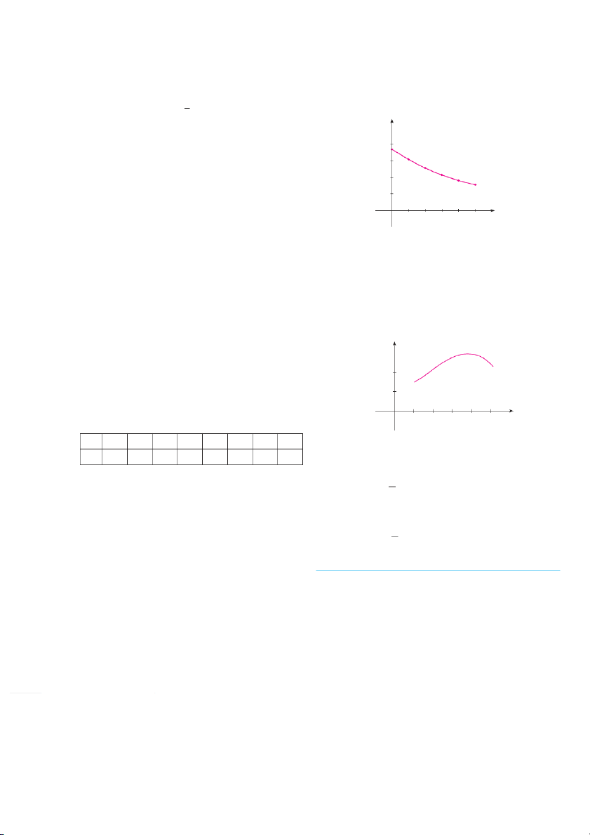
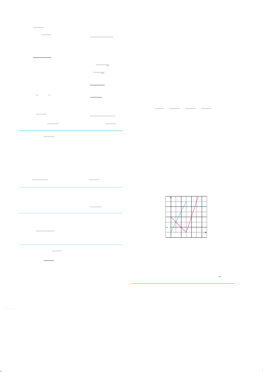
41. A warm can of soda is placed in a cold refrigerator. Sketch the
modity is C共x兲 苷 5000 ⫹ 10x ⫹ . 0.05x 2
graph of the temperature of the soda as a function of time. Is
(a) Find the average rate of change of C with respect to x
the initial rate of change of temperature greater or less than
when the production level is changed
the rate of change after an hour? ( i) from x 苷 t 100 o x 苷 105 ( ii) from x 苷 t 100 o x 苷 101
42. A roast turkey is taken from an oven when its temperature has
(b) Find the instantaneous rate of change of C with respect to
reached 185°F and is placed on a table in a room where the x when x 苷 .
100 (This is called the marginal cost. Its sig-
temperature is 75°F. The graph shows how the temperature of
nificance will be explained in Section 2.7.)
DERIVATIVES AND RATES OF CHANGE 113
46. If a cylindrical tank holds 100,000 gallons of water, which can
the oxygen content of water.) The graph shows how oxygen
be drained from the bottom of the tank in an hour, then Torri-
solubility S varies as a function of the water temperature . T
celli’s Law gives the volume V of water remaining in the tank
(a) What is the meaning of the derivative S ? 共 W T h 兲 at are its after t minutes as units?
(b) Estimate the value of S 共 an 16 d 兲interpret it. V t 共 兲 苷 100,000 (1 1 t)2 60 0 t 60 S
Find the rate at which the water is flowing out of the tank (the (mg/ L)
instantaneous rate of change of V with respect to )t as a func- 16
tion of t. What are its units? For times t 苷 0, 10, 20, 30, 40, 50,
and 60 min, find the flow rate and the amount of water remain- 12
ing in the tank. Summarize your findings in a sentence or two. 8
At what time is the flow rate the greatest? The least? 4
47. The cost of producing x ounces of gold from a new gold mine is C 苷 f 共d x oll 兲 ars. 0 8 16 24 32 40 T (°C)
(a) What is the meaning of the derivative f ? 共 W x h 兲 at are its units? Adapted from
Environmental Science: Living Within the Syst
of Nature, 2d ed.; by Charles E. Kupchella, © 1989. Reprinte
(b) What does the statement f 共800兲 m 苷 ean 17 ?
permission of Prentice-Hall, Inc., Upper Saddle River, NJ.
(c) Do you think the values of f w 共xill 兲 increase or decrease
in the short term? What about the long term? Explain.
52. The graph shows the influence of the temperature T on the
48. The number of bacteria after
maximum sustainable swimming speed S of Coho salmon.
t hours in a controlled laboratory 共T兲 experiment is
(a) What is the meaning of the derivative S ? What are n 苷 f . 共t兲
(a) What is the meaning of the derivative its units? f ? 共 Wh 兲 5 at are its S 共 兲 15 兲 units? (b) Estimate the values of and S 共 an 25 d interpret them.
(b) Suppose there is an unlimited amount of space and
nutrients for the bacteria. Which do you think is larger, S for f 共 共 兲 5 ? If t 兲 10
he supply of nutrients is limited, would (cm/s)
that affect your conclusion? Explain. 20 49. Let T bet 共 th 兲 e temperature ( in ) i
F n Phoenix thours after
midnight on September 10, 2008. The table shows values of
this function recorded every two hours. What is the meaning of T ? 共 Es 兲 8 timate its value. 0 20 T (°C) 10 t 0 2 4 6 8 10 12 14 T 82 75 74 75 84 90 93 94
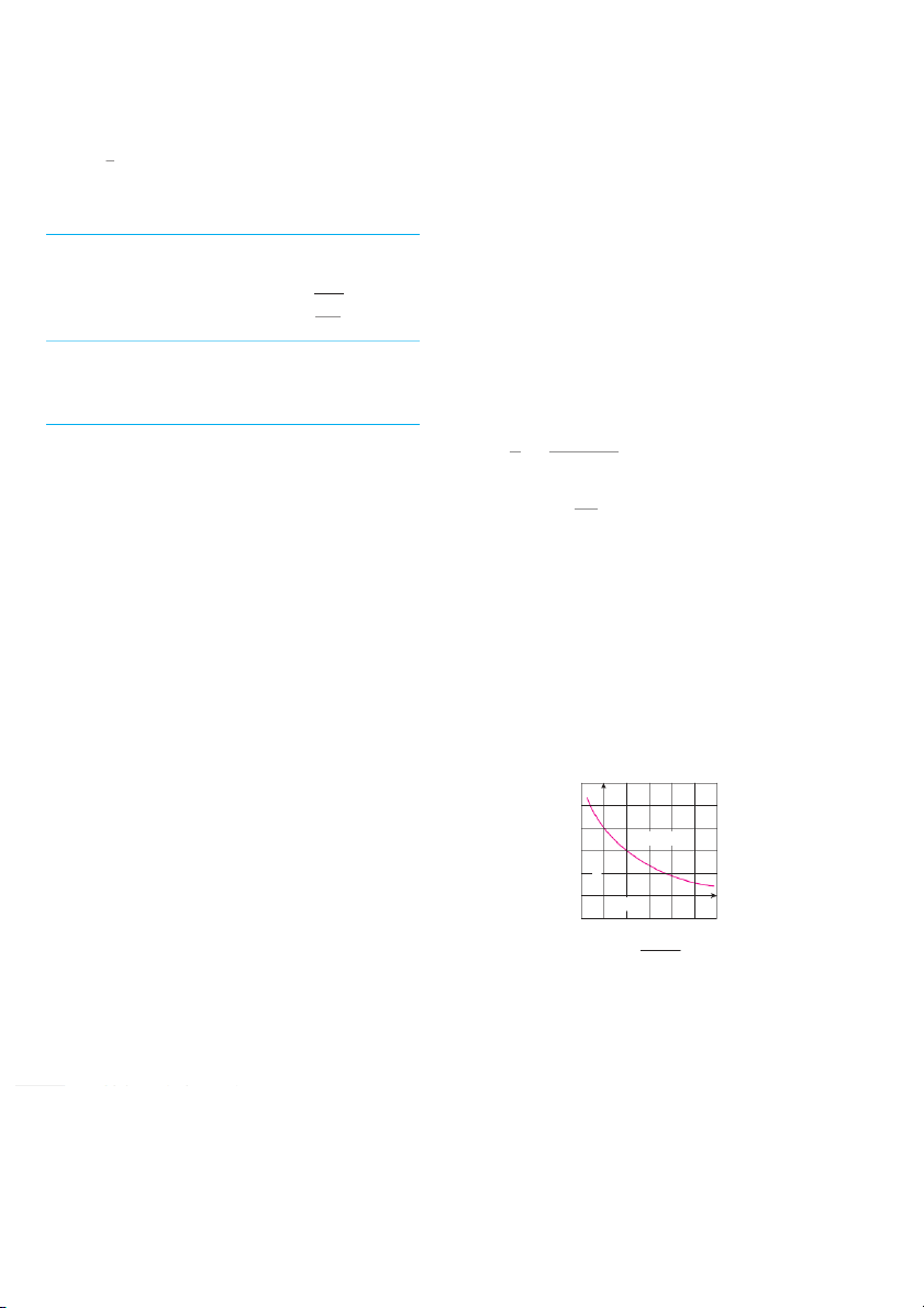
53–54 Determine whether f e 共 xis 兲 0 ts.
50. The quantity ( in pounds) of a gourmet ground coffee that is 1 if x 苷 0
sold by a coffee company at a price of p dollars per pound
53. f 共x兲 苷 再xsin x is Q 苷 f . 共 p兲 0 if x 苷 0
(a) What is the meaning of the derivative f ? 共 Wh 兲 8 at are its units? 1 (b) Is f p 共 osi 兲 8 tive or negative? Explain.
再x2 sin if x苷0
54. f 共x兲 苷 x
51. The quantity of oxygen that can dissolve in water depends on 0 if x 苷 0
the temperature of the water. (So thermal pollution influences 114 CHAPTER 2 W R I T I N G P R O J E C T
EARLY METHODS FOR FINDING TANGENTS
The first person to formulate explicitly the ideas of limits and derivatives was Sir Isaac Newton in
the 1660s. But Newton acknowledged that “If I have seen further than other men, it is because I
have stood on the shoulders of giants.” Two of those giants were Pierre Fermat (1601–1665) and
Newton’s mentor at Cambridge, Isaac Barrow (1630–1677). Newton was familiar with the meth-
ods that these men used to find tangent lines, and their methods played a role in Newton’s eventual formulation of calculus.
The following references contain explanations of these methods. Read one or more of the
references and write a report comparing the methods of either Fermat or Barrow to modern
methods. In particular, use the method of Section 2.1 to find an equation of the tangent line to the
curve y 苷 x 3 ⫹ 2x at the point (1, 3) and show how either Fermat or Barrow would have solved
the same problem. Although you used derivatives and they did not, point out similarities between the methods.
1. Carl Boyer and Uta Merzbach, A History of Mathematics (New York: Wiley, 1989), pp. 389, 432.
2. C. H. Edwards, The Historical Development of the Calculus (New York: Springer-Verlag, 1979), pp. 124, 132.
3. Howard Eves, An Introduction to the History of Mathematics, 6th ed. (New York: Saunders, 1990), pp. 391, 395.
4. Morris Kline, Mathematical Thought from Ancient to Modern Times (New York: Oxford
University Press, 1972), pp. 344, 346. 2.2 The Derivative as a Function
In the preceding section we considered the derivative of a function f at a fixed number a: f a ⫹ h ⫺ f a 1 . f ⬘ a 苷 lim h l 0 h
Here we change our point of view and let the number a vary. If we replace a in Equation 1
by a variable x, we obtain f x ⫹ h ⫺ f x 2 f ⬘ x 苷 lim h l 0 h
Given any number x for which this limit exists, we assign to x the number f ⬘ . S x o we can regard f a
⬘ s a new function, called the derivative of a
f nd defined by Equation 2. We know that the value of f a ⬘ t , x f , ⬘ ca
x n be interpreted geometrically as the slope of the tangent
line to the graph of f at the point x, f .x The function f is
⬘ called the derivative of bfecause it has been “derived” from bfy the
limiting operation in Equation 2. The domain of f i ⬘s the set xf ⬘ e x xists and may be
smaller than the domain of f. THE DERIVATIVE AS A FUNCTION 115 y
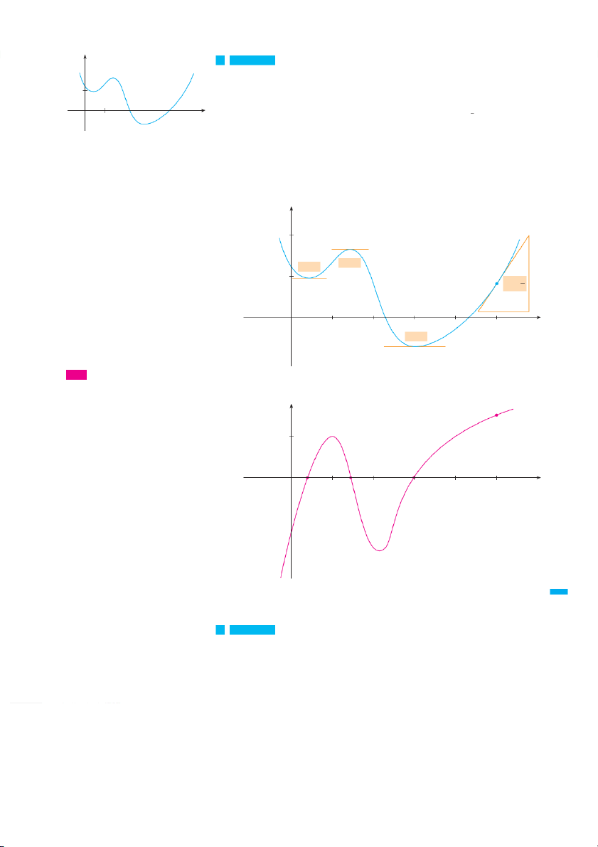
v EXAMPLE 1The graph of a function isf given in Figure 1. Use it to sketch the graph of the derivative f . ⬘ y=ƒ 1
SOLUTION We can estimate the value of the derivative at any value of x by drawing the
tangent at the point x, f xand estimating its slope. For instance, for x 苷 5 we draw 0 x
the tangent at P in Figure 2(a) and estimate its slope to be about 3, so f ⬘ 5 . Th 1.5 is 2 1
allows us to plot the point P⬘ o 5, 1.5n the graph of difrec
⬘ tly beneath P. Repeating
this procedure at several points, we get the graph shown in Figure 2(b). Notice that the FIGURE 1
tangents at A , B , and C are horizontal, so the derivative is 0 there and the graph of f ⬘ crosses the -
x axis at the points A , ⬘ ,B an ⬘ d , d C ir
⬘ectly beneath A, B, and C. Between A
and B the tangents have positive slope, so f ⬘ is
x positive there. But between and B C
the tangents have negative slope, so f ⬘ is x negative there. y B m=0 m=0 1 y=ƒ A P mÅ 32 0 x 1 5 m=0 C
TEC Visual 2.2 shows an animation of (a)
Figure 2 for several functions. y Pª(5, 1.5) y=fª(x) 1 Aª Bª Cª 0 x 1 5 FIGURE 2 (b) v EXAMPLE 2 (a) If f x 苷 ,x 3fin ⫺d
x a formula for f ⬘ .x
(b) Illustrate by comparing the graphs of a f nd f . ⬘ 116 CHAPTER 2 2 SOLUTION
(a) When using Equation 2 to compute a derivative, we must remember that the variable f
is h and that x is temporarily regarded as a constant during the calculation of the limit. _2 2 f x h f x x h 3 x h x 3 x f x 苷 lim 苷 lim h l 0 h h l 0 h 3 _2 苷 x 3 3x 2h xh2 h 3 x h x 3 x lim h l 0 h 2 苷 3x 2h 3xh2 h 3 h lim fª h l 0 h _2 2 苷 lim 3x2 3xh h 2 1 苷 3x2 1 h l 0
(b) We use a graphing device to graph f and f in Figure 3. Notice that f x wh 苷 e0n _2
f has horizontal tangents and f is
x positive when the tangents have positive slope. So FIGURE 3
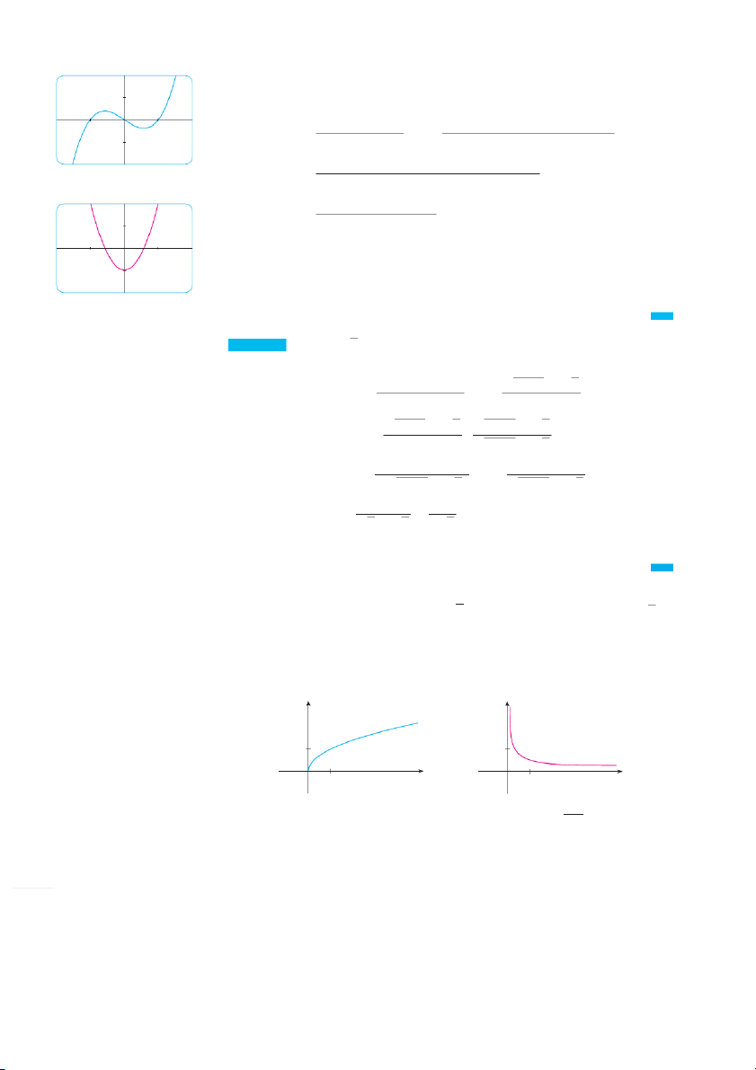
these graphs serve as a check on our work in part (a). EXAMPLE 3If f x , 苷 fisn
x d the derivative of . Sta
f te the domain of . f SOLUTION f x h f x sx h sx f x 苷 lim 苷 lim h l 0 h h l 0 h sx h s
Here we rationalize the numerator. 苷 s x lim x h sx ⴢ h l 0 h sx h sx 苷 x h x 1 lim 苷 lim h l 0 h (sx h sx ) h l 0 sx h sx 苷 1 苷 1 sx sx 2 sx We see that f e x xists if x , so 0 the domain of is f . T 0, his is smaller than the
domain of f , which is 0, .
Let’s check to see that the result of Example 3 is reasonable by looking at the graphs of
f and f in Figure 4. When i
xs close to 0, sx is also close to , 0 so f x 苷( 1 2 sx ) is
very large and this corresponds to the steep tangent lines near 0, 0 in Figure 4(a) and the large values of f j
x ust to the right of 0 in Figure 4(b). When is l x arge, f is ve x ry small
and this corresponds to the flatter tangent lines at the far right of the graph of f and the
horizontal asymptote of the graph of f . y y 1 1 0 x 0 1 x 1 FIGURE 4 (a) ƒ=œ „ x 1 (b) f ª (x)= 2œ„x THE DERIVATIVE AS A FUNCTION 117 1 x
EXAMPLE 4 Find f if f x 苷 . 2 x SOLUTION 1 x h 1 x f x h f x 2 x h 2 x f x 苷 lim 苷 lim h l 0 h h l 0 h a c - b d ad-bc 苷 1 x h 2 x 1 x 2 x h lim = § 1 h l 0 e bd e h 2 x h 2 x 苷 2 x 2h x 2 xh 2 x h x 2 xh lim h l 0 h 2 x h 2 x 苷 3h lim h l 0 h 2 x h 2 x 苷 3 lim 苷 3 h l 0 2 x h 2 x 2 x 2 Other Notations Leibniz
If we use the traditional notation y 苷 f t
x o indicate that the independent variable is an xd
Gottfried Wilhelm Leibniz was born in Leipzig t he dependent variable is y, then some common alternative notations for the derivative are
in 1646 and studied law, theology, philosophy, as follows:
and mathematics at the university there, gradu-
ating with a bachelor’s degree at age 17. After dy
earning his doctorate in law at age 20, Leibniz f x
苷 y 苷苷 df 苷 d f x 苷 Df x 苷 Dx f x dx dx dx
entered the diplomatic service and spent most
of his life traveling to the capitals of Europe on The symbols
political missions. In particular, he worked to
D and d dxare called differentiation operators because they indicate the
avert a French military threat against Ger many operation of differentiatio ,
n which is the process of calculating a derivative.
and attempted to reconcile the Catholic and
The symbol dy d ,x which was introduced by Leibniz, should not be regarded as a ratio Protestant churches.
(for the time being); it is simply a synonym for f . N
x onetheless, it is a very useful and
His serious study of mathematics did not
suggestive notation, especially when used in conjunction with increment notation. Referring
begin until 1672 while he was on a diplomatic to Equation 2.1.6, we can rewrite the definition of derivative in Leibniz notation in the form
mission in Paris. There he built a calculating
machine and met scientists, like Huygens, who
directed his attention to the latest develop - dy
ments in mathematics and science. Leibniz 苷 y lim dx x l 0 x
sought to develop a symbolic logic and system
of notation that would simplify logical reason-
ing. In particular, the version of calculus that I
he f we want to indicate the value of a derivative dy dxin Leibniz notation at a specific num-
published in 1684 established the notation and ber a, we use the notation
the rules for finding derivatives that we use today.
Unfortunately, a dreadful priority dispute dy dy or
arose in the 1690s between the followers of dx x苷a dx x苷a
Newton and those of Leibniz as to who had
invented calculus first. Leibniz was even
which is a synonym for f .a
accused of plagiarism by members of the Royal
Society in England. The truth is that each man
invented calculus independently. Newton
arrived at his version of calculus first but,
3 Definition A function f is differentiable at a if f e
a xists. It is differen-
because of his fear of controversy, did not pub-
tiable on an open interval a, b[or a o , r or , a ] if it i , s differ-
lish it immediately. So Leibniz’s 1684 account
entiable at every number in the interval.
of calculus was the first to be published. 118 CHAPTER 2
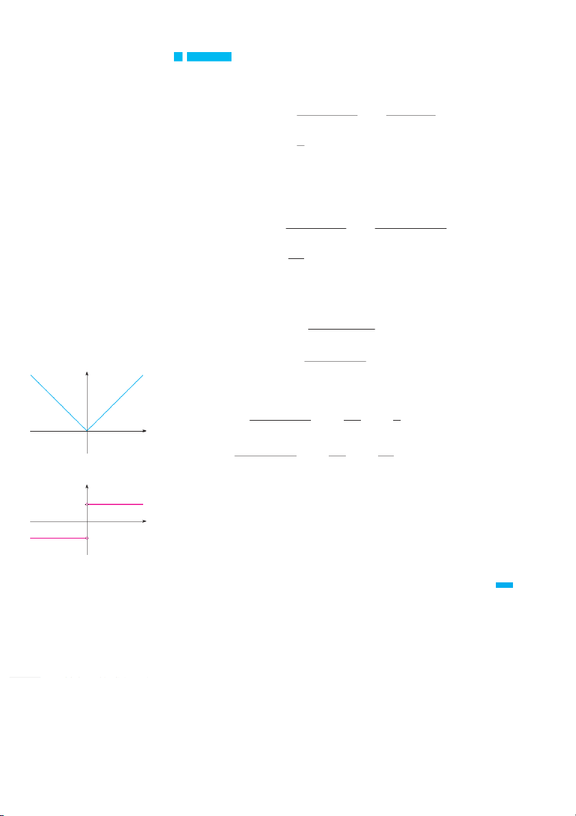
v EXAMPLE 5Where is the function f x 苷x differentiable? SOLUTION If x
0 , then x 苷 x and we can choose
h small enough that x h 0 and hence x h 苷 x .
h Therefore, for x 0, we have x h x x h x f x 苷 lim 苷 lim h l 0 h h l 0 h 苷 h lim 苷 lim1 苷 1 h l 0 h h l 0
and so f is differentiable for any x 0 . Similarly, for x 0 we have x 苷
x and h can be chosen small enough that x h 0 and so x h 苷 x .
h Therefore, for x 0, x h x x h x f x 苷 lim 苷 lim h l 0 h h l 0 h 苷 h lim 苷 lim 1 苷 1 h l 0 h h l 0
and so f is differentiable for any x 0 .
For x 苷 0 we have to investigate f 0 h f 0 f 0 苷 lim h l 0 h 苷 0 h 0 lim if it exists h l 0 h y
Let’s compute the left and right limits separately: 0 h 0 h h lim 苷 lim 苷 lim 苷 lim1 苷 1 h l0 h h l 0 h h l0 h h l 0 0 x 0 h 0 h h and lim 苷 lim 苷 lim 苷 lim 1 苷 1 h l0 h h l 0 h h l0 h h l 0 (a) y=ƒ=| x | y
Since these limits are different, f d
0 oes not exist. Thus f is differentiable at all x except 0. 1
A formula for f is given by 0 x if x 0 f x 苷 1 _1 1 if x 0
and its graph is shown in Figure 5(b). The fact that f d
0 oes not exist is reflected geo- (b) y=f ª(x)
metrically in the fact that the curve y 苷x does not have a tangent line at . 0, 0 [See FIGURE 5 Figure 5(a).]
Both continuity and differentiability are desirable properties for a function to have. The
following theorem shows how these properties are related. THE DERIVATIVE AS A FUNCTION 119
4 Theorem If f is differentiable at a , then f is continuous at a .
PROOF To prove that f is continuous at a , we have to show that li f mx l a x 苷 f . W a e
do this by showing that the difference f x ⫺ f ap a proaches 0.
The given information is that f is differentiable at , a that is, f x ⫺ f a f ⬘ a 苷 lim x l a x ⫺ a
PS An important aspect of problem solving is exists (see Equation 2.1.5). To connect the given and the unknown, we divide and multi-
trying to find a connection between the given ply f x ⫺ f by
a x ⫺ a (which we can do when x 苷 ) a :
and the unknown. See Step 2 (Think of a Plan)
in Principles of Problem Solving on page 97. f x ⫺ f a 苷 f x ⫺ f a x ⫺ a x ⫺ a
Thus, using the Product Law and (2.1.5), we can write f x ⫺ f a lim f x ⫺ f a 苷 lim x ⫺ a x l a x l a x ⫺ a 苷 f x ⫺ f a lim ⴢ lim x ⫺ a x l a x ⫺ a x l a
苷 f ⬘ a ⴢ 0 苷 0
To use what we have just proved, we start with f an
x d add and subtract f : a limf x
苷 lim f a ⫹ f x ⫺ f a x l a x l a
苷 limf a ⫹ lim f x ⫺ f a x l a x l a
苷 f a ⫹ 0 苷 f a
Therefore f is continuous at a. |
NOTE The converse of Theorem 4 is false; that is, there are functions that are contin-
uous but not differentiable. For instance, the function f x
苷x is continuous at 0 because limf x
苷 limx 苷 0 苷 f 0 x l 0 x l 0
(See Example 7 in Section 1.6.) But in Example 5 we showed that f is not differentiable at 0.
How Can a Function Fail to Be Differentiable?
We saw that the function y 苷 x in Example 5 is not differentiable at 0 and Figure 5(a)
shows that its graph changes direction abruptly when x 苷 .
0 In general, if the graph of a
function f has a “corner” or “kink” in it, then the graph of f has no tangent at this point
and is fnot differentiable there. [In trying to compute f ⬘ , awe find that the left and right limits are different.] 120 CHAPTER 2 y
Theorem 4 gives another way for a function not to have a derivative. It says that if f is vertical tangent
not continuous at a, then f is not differentiable at .
a So at any discontinuity (for instance, line
a jump discontinuity) f fails to be differentiable.
A third possibility is that the curve has a vertical tangent line when x 苷 ; a that is, f is continuous at a and lim f x 苷 x l a 0 a x
This means that the tangent lines become steeper and steeper as x l a . Figure 6 shows one
way that this can happen; Figure 7(c) shows another. Figure 7 illustrates the three possi-
bilities that we have discussed. FIGURE 6 y y y 0 a x 0 a x 0 a x FIGURE 7 Three ways for ƒ not to be differentiable at a (a) A corner (b) A discontinuity (c) A vertical tangent
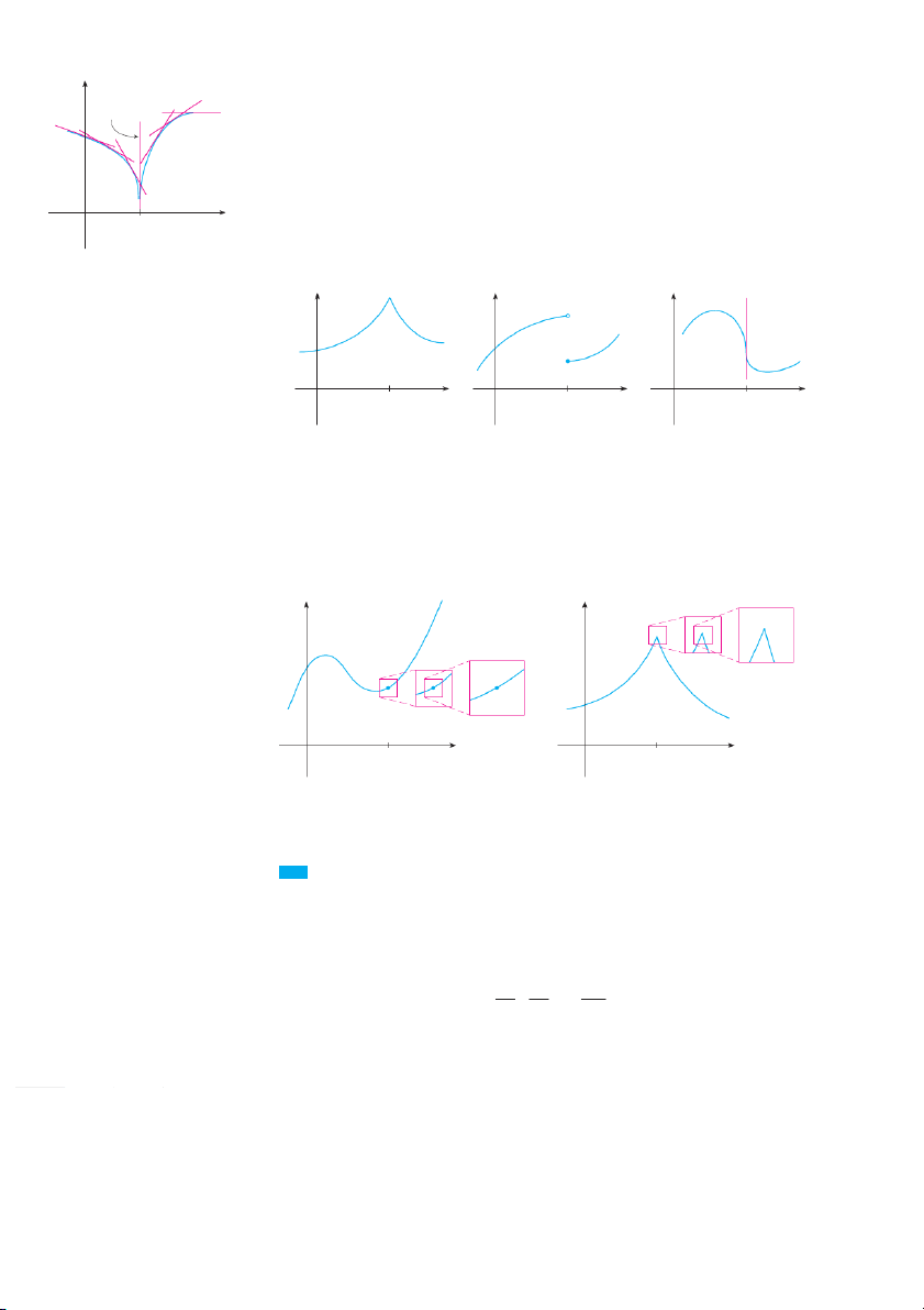
A graphing calculator or computer provides another way of looking at differentiabil- ity. If is d
f ifferentiable at , the
a n when we zoom in toward the point a, f a the graph
straightens out and appears more and more like a line. (See Figure 8. We saw a specific
example of this in Figure 2 in Section 2.1.) But no matter how much we zoom in toward a
point like the ones in Figures 6 and 7(a), we can’t eliminate the sharp point or corner (see Figure 9). y y 0 x a 0 x a FIGURE 8 FIGURE 9
ƒ is differentiable at a.
ƒ is not differentiable at a. Higher Derivatives If is
f a differentiable function, then its derivative f is also a function, so f may have a
derivative of its own, denoted by f . Th
苷 ifs new function f is called the second
derivative of f because it is the derivative of the derivative of f . Using Leibniz notation,
we write the second derivative of y 苷 f x as d dy d 2y 苷 dx dx dx2 THE DERIVATIVE AS A FUNCTION 121 EXAMPLE 6 If f x , 苷 fxin 3 d an x d interpret f . x 2
SOLUTION In Example 2 we found that the first derivative is f x 苷 3x2 . S1o the f · second derivative is fª f f x h f x 3 x h 2 1 3x 2 1 _1.5 1.5 f x 苷 f x 苷 lim 苷 lim h l 0 h h l 0 h 苷 3x 2 6xh 3h2 1 3x 2 1 lim
苷 lim 6x 3h 苷 6x h l 0 h h l 0 _2 FIGURE 10
The graphs of f , f , and f are shown in Figure 10. We can interpret f a
x s the slope of the curve y 苷 f at the x point . I x n , f x
other words, it is the rate of change of the slope of the original curve y 苷 f .x Notice from Figure 10 that TEC f is x negative when y 苷 f has n x egative slope
In Module 2.2 you can see how changing f and positive when
the coefficients of a polynomial affects the y 苷 f h
xas positive slope. So the graphs serve as a check on our
appearance of the graphs of , f f , and f . calculations.
In general, we can interpret a second derivative as a rate of change of a rate of change.
The most familiar example of this is acceleration, which we define as follows.
If s 苷 s its the position function of an object that moves in a straight line, we know that
its first derivative represents the velocity v t of the object as a function of time: v t 苷 s t 苷 ds dt
The instantaneous rate of change of velocity with respect to time is called the acceleration
a t of the object. Thus the acceleration function is the derivative of the velocity function
and is therefore the second derivative of the position function: a t 苷 v t 苷 s t or, in Leibniz notation,
a 苷 dv 苷 d 2s dt dt2
The third derivative f
is the derivative of the second derivative: f 苷 f . So f c
x an be interpreted as the slope of the curve y 苷 f or a
x s the rate of change of f . I x f y 苷 ,f the
x n alternative notations for the third derivative are d 2 y y 苷 f x 苷 d 苷 d3y dx dx2 dx3
The process can be continued. The fourth derivative f
is usually denoted by f .4 In gen-
eral, the nth derivative of f is denoted by f n and is obtained from fby differentiating n
times. If y 苷 f , x we write y n 苷 f n x 苷 dny dxn EXAMPLE 7 If f x 苷 x3 , find x f and x . f 4 x
SOLUTION In Example 6 we found that f x
苷 . 6Txhe graph of the second derivative
has equation y 苷 6x and so it is a straight line with slope 6. Since the derivative f i xs 122 CHAPTER 2 the slope of f ⬙ , 共 w x e 兲have f 共x兲 苷 6
for all values of x . So f
is a constant function and its graph is a horizontal line. There-
fore, for all values of x ,
f 共4兲共x兲 苷 0
We can also interpret the third derivative physically in the case where the function is
the position function s 苷 s共tof
兲 an object that moves along a straight line. Because s 苷 共s⬙兲 , t ⬘ he 苷thaird
⬘ derivative of the position function is the derivative of the accel-
eration function and is called the jerk:
j 苷 da 苷 d3s dt dt3
Thus the jerk j is the rate of change of acceleration. It is aptly named because a large jerk
means a sudden change in acceleration, which causes an abrupt movement in a vehicle.
We have seen that one application of second and third derivatives occurs in analyzing
the motion of objects using acceleration and jerk. We will investigate another applica-
tion of second derivatives in Section 3.3, where we show how knowledge of f g ⬙ ives us
information about the shape of the graph of f . In Chapter 11 we will see how second and
higher derivatives enable us to represent functions as sums of infinite series. 2.2 Exercises
1–2 Use the given graph to estimate the value of each derivative.
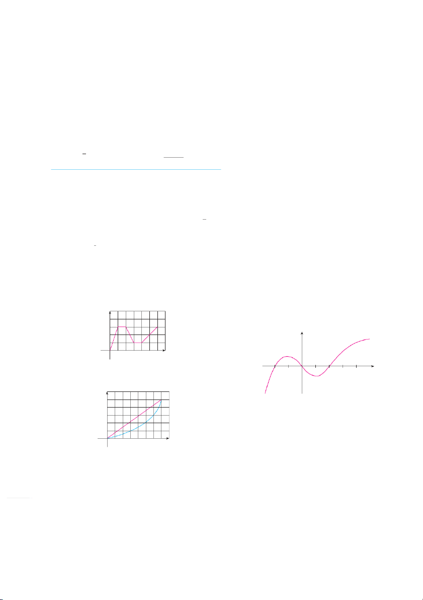
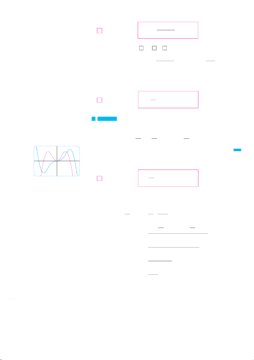
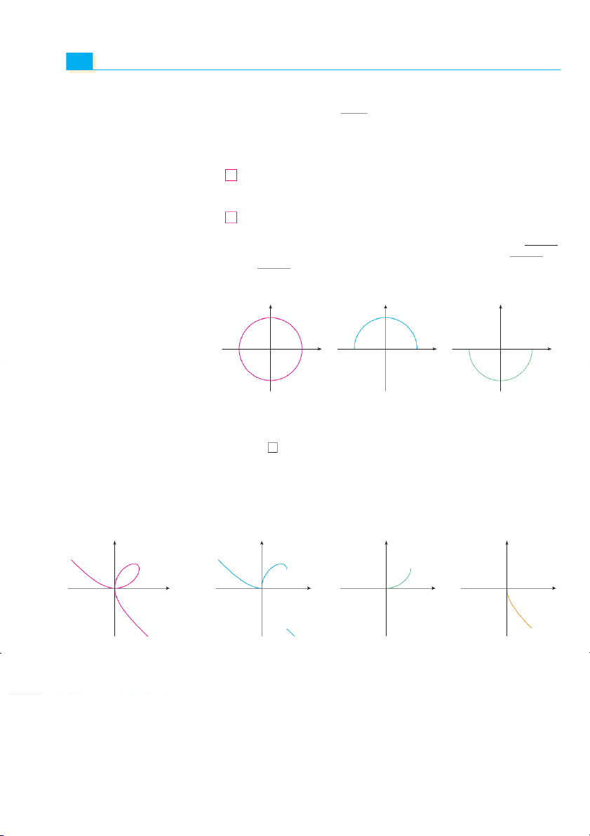
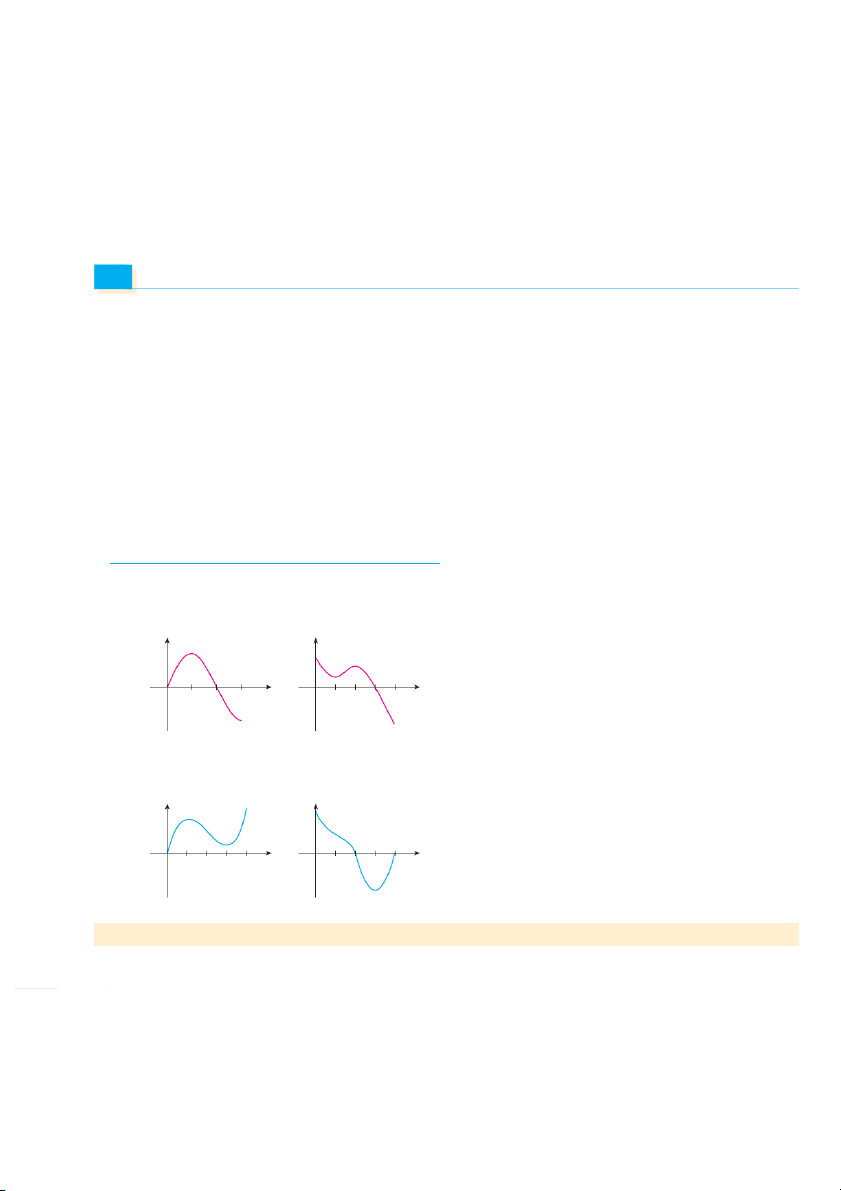
3. Match the graph of each function in (a)–(d) with the graph of
Then sketch the graph of f .⬘
its derivative in I–IV. Give reasons for your choices. 1. y y (a) f ⬘共⫺3兲 (b) f ⬘共⫺2 ( 兲 c) f ⬘共⫺ 兲 1 (a) (b) (d) f ⬘共0兲 (e) f ⬘共1兲 (f) f ⬘共 兲 2 (g) f ⬘共 兲 3 0 x 0 x y 1 y y (c) (d) 1 x 0 x 0 x 2. (a) f ⬘共0兲 (b) f ⬘共1兲 (c) f ⬘共 兲 2 I y II y (d) f ⬘共3兲 (e) f ⬘共4兲 (f) f ⬘共 兲 5 (g) f ⬘共6兲 (h) f ⬘共7兲 0 x 0 x y y y 1 III IV 0 1 x 0 x 0 x
; Graphing calculator or computer required
1. Homework Hints available at stewartcalculus.com THE DERIVATIVE AS A FUNCTION 123
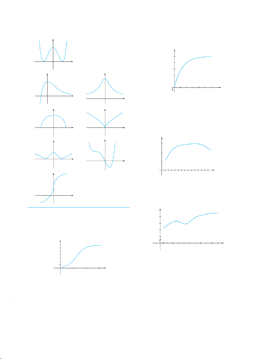
4–11 Trace or copy the graph of the given function .f (Assume that
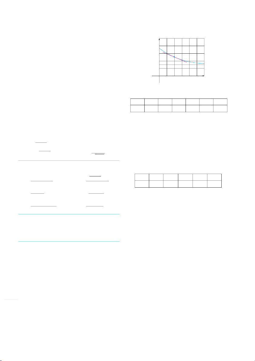
13. A rechargeable battery is plugged into a charger. The graph
the axes have equal scales.) Then use the method of Example 1 to shows C共, tthe
兲 percentage of full capacity that the battery sketch the graph of f b ⬘ elow it.
reaches as a function of time t elapsed ( in hours). 4.
(a) What is the meaning of the derivative C⬘ ? 共t兲 y
(b) Sketch the graph of C⬘ . 共W t h 兲at does the graph tell you? C 100 0 x 80 percentage 60 of full charge 5. y 6. y 40 20 t (hours) 2 4 6 8 10 12 0 x 0 x
14. The graph (from the US Department of Energy) shows how 7. 8.
driving speed affects gas mileage. Fuel economy F is measured y y
in miles per gallon and speed i
v s measured in miles per hour.
(a) What is the meaning of the derivative F⬘ ? 共v兲
(b) Sketch the graph of F⬘ . 共v兲
(c) At what speed should you drive if you want to save on gas? 0 x 0 x 9. 10. F (mi/ gal) y y 30 20 0 x 0 x 10 11. y 0 √ (mi/h) 10 20 30 40 50 60 70
15. The graph shows how the average age of first marriage of
Japanese men varied in the last half of the 20th century. 0 共t兲 x
Sketch the graph of the derivative function M⬘ . During
which years was the derivative negative? M
12. Shown is the graph of the population function P ft 共 or 兲 yeast
cells in a laboratory culture. Use the method of Example 1 to 27
graph the derivative P⬘ . W 共t ha 兲 t does the graph of tell P us ⬘ about the yeast population? 25 P (yeast cells) 1960 1970 1980 1990 2000 t 500
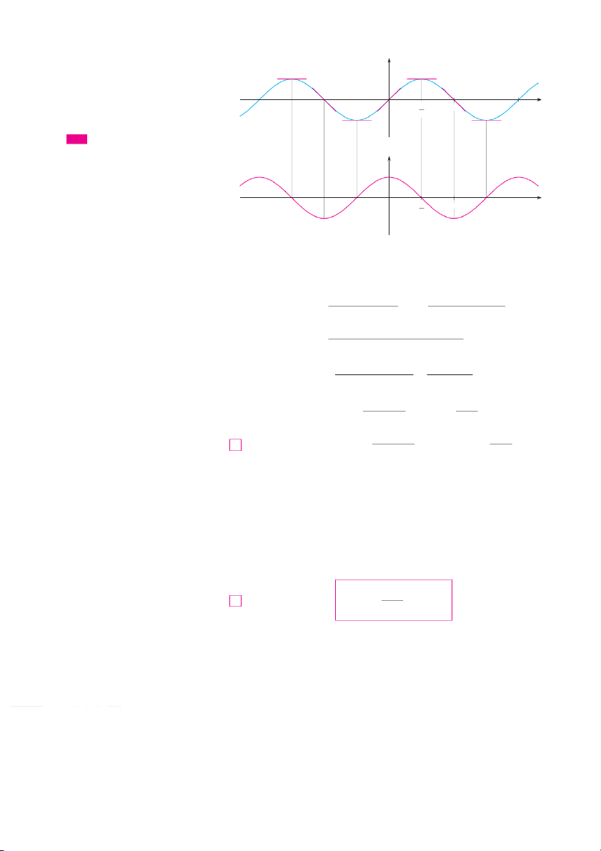
16. Make a careful sketch of the graph of the sine function and
below it sketch the graph of its derivative in the same manner 0 t
as in Exercises 4–11. Can you guess what the derivative of the (hours) 5 10 15
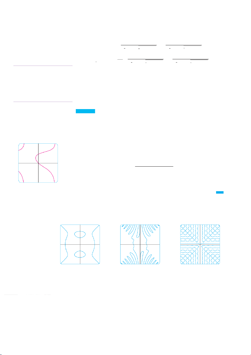
sine function is from its graph? 124 CHAPTER 2 ; 17. Let 33. U共t兲
f 共x兲 .苷 x 2 The unemployment rate varies with time. The table
(from the Bureau of Labor Statistics) gives the percentage of
(a) Estimate the values of f , 共 (1 兲 0 ) 2 , f , f and 共 f 共 兲 1 by 兲 2
unemployed in the US labor force from 1999 to 2008.
using a graphing device to zoom in on the graph of f.
(b) Use symmetry to deduce the values of ( 1f ) 2 , f 共 , 1兲 t
U共t兲 t U共t兲 and f 共 . 兲 2
(c) Use the results from parts (a) and (b) to guess a formula 1999 4.2 2004 5.5 for f . 共x兲 2000 4.0 2005 5.1
(d) Use the definition of derivative to prove that your guess 2001 4.7 2006 4.6 in part (c) is correct. 2002 5.8 2007 4.6 2003 6.0 2008 5.8
; 18. Let f 共x兲 .苷 x3
(a) What is the meaning of U ? 共W t h 兲 at are its units?
(a) Estimate the values of f , 共 (1 兲 0 ) 2 , , f f ,f an 共d 共 f兲 1 共 兲 2 兲 3
(b) Construct a table of estimated values for U . 共t兲
by using a graphing device to zoom in on the graph of f.
(b) Use symmetry to deduce the values of ( 1f ) 34. Let P共t be
兲 the percentage of Americans under the age of 18 2 , f 共 ,1兲 f , and 共 f2 共 兲 . 兲 3
at time .t The table gives values of this function in census
(c) Use the values from parts (a) and (b) to graph f . years from 1950 to 2000.
(d) Guess a formula for f . 共x兲
(e) Use the definition of derivative to prove that your guess t
P共t兲 t P共t兲 in part (d) is correct. 1950 31.1 1980 28.0 1960 35.7 1990 25.7
19–29 Find the derivative of the function using the definition of 1970 34.0 2000 25.7
derivative. State the domain of the function and the domain of its derivative.
(a) What is the meaning of P ? 共 W t h 兲 at are its units? 19. 共 f 共x兲 x 苷1 1 20. f
(b) Construct a table of estimated values for P . t兲 3 共x兲 苷 mx b 2 (c) Graph a P nd P . 21.
f 共t兲 苷 5t 9t 2
22. f 共x兲 苷 1.5x2 x 3.7
(d) How would it be possible to get more accurate values for P ? 共t兲
23. f 共x兲 苷 x2 2x 3 24. t共t兲 苷 1 s
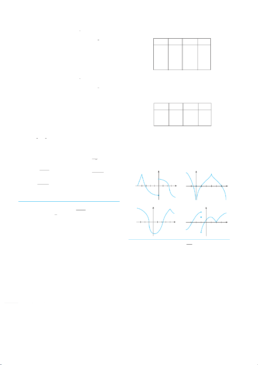
35–38 The graph of f is given. State, with reasons, the numbers t
at which f is not differentiable. 25. t共x兲 苷 s9 x 26. 35. y 36. f 共x兲 苷 x 2 1 y 2x 3 27.
28. f 共x兲 苷 x3兾2 G共t兲 苷 1 2t 0 3 t _2 0 2 x 2 4 x
29. f 共x兲 苷 x4 37. y 38. y
30. (a) Sketch the graph of f 共x兲 苷 s6 by x starting with the
graph of y 苷 sx and using the transformations of Sec - tion 1.3. 0 0
(b) Use the graph from part (a) to sketch the graph of f . _2 4 x _2 2 x
(c) Use the definition of a derivative to find f . 共 W x h 兲 at are
the domains of f and f ? ;
(d) Use a graphing device to graph fand compare with your sketch in part (b).
; 39. Graph the function f 共x兲 苷 x . s Zoom in repeatedly, ⱍx ⱍ
first toward the point ( 1, 0) and then toward the origin. 31. (a) If f 共x兲 苷 ,
x f4ind f2x . 共x兲
What is different about the behavior of f in the vicinity of ;
(b) Check to see that your answer to part (a) is reasonable by
these two points? What do you conclude about the differen-
comparing the graphs of afnd f . tiability of f ?
; 40. Zoom in toward the points (1, 0), (0, 1), and ( 1, 0) on 32. (a) If
f 共x兲 苷 ,x find 1 f兾x . 共x兲
the graph of the function t共x兲 苷 共x 2 . W 1 h 兲a2t 兾 d3o you ;
(b) Check to see that your answer to part (a) is reasonable by
notice? Account for what you see in terms of the differen-
comparing the graphs of afnd f . tiability of t.
THE DERIVATIVE AS A FUNCTION 125
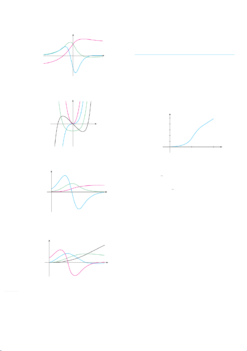
41. The figure shows the graphs of , f ,f an ⬘ d f . I ⬙ dentify each
; 45–46 Use the definition of a derivative to find an f d ⬘ f 共x . ⬙共 兲 x兲
curve, and explain your choices.
Then graph , f ,f an ⬘ d f o
⬙n a common screen and check to see if y your answers are reasonable. a
45. f 共x兲 苷 3x2 ⫹ 2x ⫹ 1 b
46. f 共x兲 苷 x3 ⫺ 3x x c ; 47. If , findf 共x ,
兲 苷 2 ,x2 ⫺ fx ,f3 ⬘an f ⬙ 共 dx 共 共x 兲 f 共4 x兲 兲 . 兲共x兲 Graph , f , f f ⬘ , a
⬙ nd f on a common screen. Are the graphs
consistent with the geometric interpretations of these derivatives?
42. The figure shows graphs of f ,f , f ⬘, an ⬙ d f . Identify each 48.
curve, and explain your choices.
(a) The graph of a position function of a car is shown, where s
is measured in feet and t in seconds. Use it to graph the a b c d
velocity and acceleration of the car. What is the accelera- y
tion at t 苷 10seconds? s x 100 0 10 t 20
43. The figure shows the graphs of three functions. One is the posi-
tion function of a car, one is the velocity of the car, and one is
(b) Use the acceleration curve from part (a) to estimate the
its acceleration. Identify each curve, and explain your choices.
jerk at t 苷 10seconds. What are the units for jerk? y a
49. Let f 共x兲 苷 3 x.s b c (a) If a, us
苷 e 0Equation 2.1.5 to find f ⬘ . 共 兲 a (b) Show that f ⬘ d 共 oes 兲 0 not exist. (c) Show that y 苷 3 x h
s as a vertical tangent line at 共 . 兲 0, 0 0 t
(Recall the shape of the graph of f. See Figure 13 in Section 1.2.) 50. (a) If t共x , 兲 sh 苷ow x 2 t 兾 h3at t⬘共does 兲 0 not exist. (b) If a, fin 苷 d0 t⬘ . 共 兲 a
44. The figure shows the graphs of four functions. One is the (c) Show that y 苷 h x a 2 s 兾 a
3 vertical tangent line at 共 . 兲 0, 0
position function of a car, one is the velocity of the car, one is ;
(d) Illustrate part (c) by graphing y 苷 x.2兾3
its acceleration, and one is its jerk. Identify each curve, and explain your choices.
51. Show that the function f 共x兲 苷 is not differentiable ⱍx ⫺ 6 ⱍ y
at 6. Find a formula for f a ⬘nd sketch its graph. d a b c
52. Where is the greatest integer function f 共x兲 苷 no 冀t xdif 冁feren-
tiable? Find a formula for f an ⬘ d sketch its graph. 0 t
53. (a) Sketch the graph of the function f 共x兲 苷x . ⱍ xⱍ
(b) For what values of x is f differentiable?
(c) Find a formula for f . ⬘ 126 CHAPTER 2
54. The left-hand and right-hand derivatives of f at a are defined
(c) Where is f discontinuous? by
(d) Where is f not differentiable? f 共a h兲 f 共 兲 a
55. Recall that a function is callfed even if f 共 x兲 苷 f fo 共r xall 兲
f 共a兲 苷 lim x 共 兲 h l 0 h
in its domain and odd if f 共 x兲 苷 f for a x ll such . x Prove each of the following. f 共a h兲 f 共 兲 a and
(a) The derivative of an even function is an odd function.
f 共a兲 苷 lim h l 0 h
(b) The derivative of an odd function is an even function. 56. if these limits exist. Then
When you turn on a hot-water faucet, the temperature T of the f e 共 xis 兲 a ts if and only if these one-
sided derivatives exist and are equal.
water depends on how long the water has been running. (a) Find
(a) Sketch a possible graph of T as a function of the time t that f 共 a 4 nd 兲 f 共 f 4 or 兲 the function
has elapsed since the faucet was turned on. 0
(b) Describe how the rate of change of T with respect to if t x 0 varies as t increases. 5 x if 0 x 4 f 共x兲 苷
(c) Sketch a graph of the derivative of . T 1 if x 4
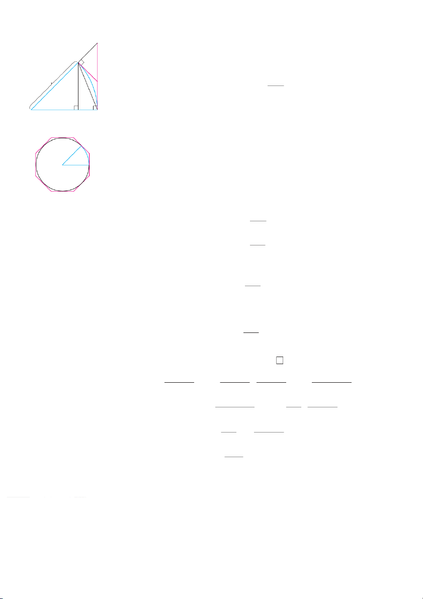
57. Let ᐍ be the tangent line to the parabola y 苷 x 2 at the point 5 x 共 . 1, 1 Th
兲 e angle of inclination of is th ᐍ e angle that ᐍmakes
with the positive direction of the x-axis. Calculate correct to
(b) Sketch the graph of f. the nearest degree. 2.3 Differentiation Formulas
If it were always necessary to compute derivatives directly from the definition, as we did
in the preceding section, such computations would be tedious and the evaluation of some
limits would require ingenuity. Fortunately, several rules have been developed for finding y
derivatives without having to use the definition directly. These formulas greatly simplify the task of differentiation. c y=c
Let’s start with the simplest of all functions, the constant function f 共x兲 . T 苷 hce graph slope=0
of this function is the horizontal line y 苷 c, which has slope 0, so we must have f 共x兲 .苷 0
(See Figure 1.) A formal proof, from the definition of a derivative, is also easy: f 共x h兲
f 共x兲 c c 0 x
f 共x兲 苷 lim 苷 lim 苷 lim0 苷 0 h l 0 h h l 0 h h l 0 FIGURE 1
In Leibniz notation, we write this rule as follows. The graph of ƒ=c is the line y=c, so fª(x)=0.
Derivative of a Constant Function d 共c兲 苷 0 y dx y=x slope=1 Power Functions
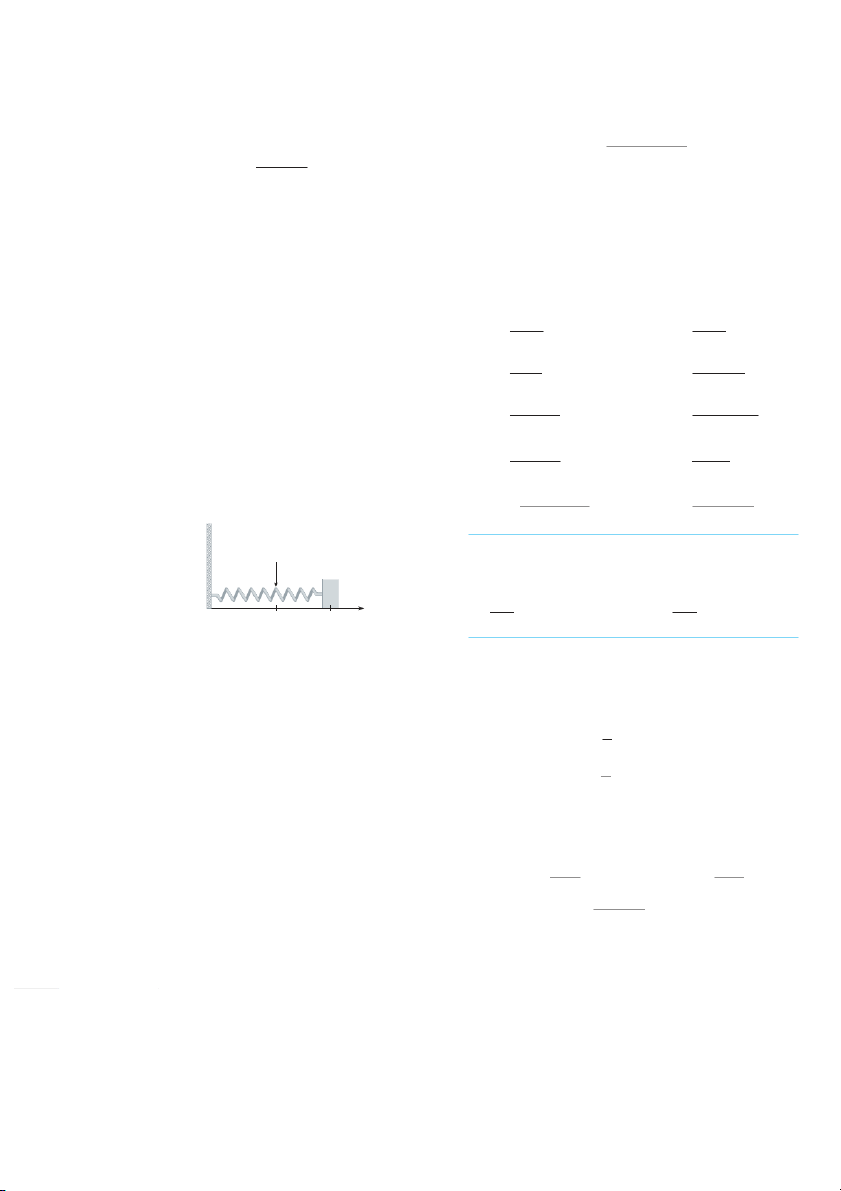
We next look at the functions f 共x兲 , 苷 w x h
n ere n is a positive integer. If n , t 苷he 1 graph 0 of f 共x兲 is
苷 txhe line y 苷 x, which has slope 1. (See Figure 2.) So x FIGURE 2 d 1 共x兲 苷 1 The graph of ƒ=x is the dx line y=x, so fª(x)=1. DIFFERENTIATION FORMULAS 127
(You can also verify Equation 1 from the definition of a derivative.) We have already
investigated the cases n 苷 2 and n 苷 3. In fact, in Section 2.2 (Exercises 17 and 18) we found that d 2 共 d x 2 兲 苷 2x 共x3兲 苷 3x2 dx dx
For n 苷 4 we find the derivative of f 共x兲 a 苷 sx f4ollows: f 共x h兲
f 共x兲 共x h兲4 x 4
f 共x兲 苷 lim 苷 lim h l 0 h h l 0 h 4 2 4 苷 x 4x 3h x 6 2h 4xh3 h x 4 lim h l 0 h 苷 4x 3h 6x 2h 2 4xh3 h 4 lim h l 0 h 苷 lim共4x3 6x 2h 4xh2 h 3 兲 苷 4x 3 h l 0 Thus d 3 共x4兲 苷 4x3 dx
Comparing the equations in 1 , 2 , and 3 , we see a pattern emerging. It seems to be a rea-
sonable guess that, when n is a positive integer, 共d兾dx兲共x n 兲 . T 苷 hi n s
x ntu1rns out to be
true. We prove it in two ways; the second proof uses the Binomial Theorem.
The Power Rule If n is a positive integer, then
d 共xn兲 苷 nxn 1 dx FIRST PROOF The formula x n a n 苷 共x a兲共x n 1 x n 2a xa n 2 a n 1 兲
can be verified simply by multiplying out the right-hand side (or by summing the second
factor as a geometric series). If f 共x兲 ,
苷 wxen can use Equation 2.1.5 for f and 共 tahe 兲 equation above to write f 共x兲 f a 共 兲 xn a n
f 共a兲 苷 lim 苷 lim x l a x a x l a x a 苷 lim共xn 1 x n 2a xa n 2 a n 1 兲 x l a 苷 an 1 a n 2a aan 2 a n 1 苷 nan 1 128 CHAPTER 2 SECOND PROOF f x h f x x h n x n f x 苷 lim 苷 lim h l 0 h h l 0 h
The Binomial Theorem is given on
In finding the derivative of x 4 we had to expand x h . H 4 ere we need to expand Reference Page 1. x h an
n d we use the Binomial Theorem to do so: n n 1 x n nxn 1h x n 2h 2 nxh n 1 h n x n 2 f x 苷 lim h l 0 h n n 1 nxn 1h x n 2h 2 nxh n 1 h n 苷 2 lim h l 0 h 苷 lim n n 1 n x n 1 x n 2h nxh n 2 h n 1 h l 0 2 苷 nxn 1
because every term except the first has h as a factor and therefore approaches 0.
We illustrate the Power Rule using various notations in Example 1. EXAMPLE 1 (a) If f x 苷, txh6en f x .苷 6x 5 (b) If y , t 苷 he x n 1000 苷 y . 1000x 999 dy d
(c) If y 苷 t ,4 then 苷 4t .3 (d) r 3 苷 3r2 dt dr New Derivatives from Old
When new functions are formed from old functions by addition, subtraction, or multiplica-
tion by a constant, their derivatives can be calculated in terms of derivatives of the old func-
tions. In particular, the following formula says that the derivative of a constant times a
function is the constant times the derivative of the function. GEOMETRIC INTERPRETATION OF THE CONSTANT MULTIPLE RULE
The Constant Multiple Rule If c is a constant and f is a differentiable function, then y d d c f x 苷 cf x dx dx y=2ƒ y=ƒ PROOF Let
t x 苷 cf . xThen 0 x t x h t x c f x h c f x t x 苷 lim 苷 lim h l 0 h h l 0 h Multiplying by c 苷 2 stretches the graph verti-
cally by a factor of 2. All the rises have been 苷 lim f x h f x
doubled but the runs stay the same. So the c h l 0 h slopes are doubled too. 苷 f x h f x c lim (by Law 3 of limits) h l 0 h 苷 cf x DIFFERENTIATION FORMULAS 129 EXAMPLE 2 d d (a) 3x 4 苷 3 x 4
苷 3 4x3 苷 12x3 dx dx d d (b) x 苷d 1 x 苷 1 x 苷 1 1 苷 1 dx dx dx
The next rule tells us that the derivative of a sum of functions is the sum of the derivatives.
The Sum Rule If f and t are both differentiable, then
Using prime notation, we can write the Sum Rule as d d d f t 苷 f t f x t x 苷 f x t x dx dx dx
PROOF Let F x 苷 f x . t Thxen F x h F x F x 苷 lim h l 0 h 苷 f x h t x h f x t x lim h l 0 h 苷 t x h t x lim f x h f x h l 0 h h 苷 f x h f x t x h t x lim lim (by Law 1) h l 0 h h l 0 h 苷 f x t x
The Sum Rule can be extended to the sum of any number of functions. For instance,
using this theorem twice, we get f t h 苷 f t h 苷 f t h 苷 f t h By writing f t as f
1 atnd applying the Sum Rule and the Constant Multiple
Rule, we get the following formula.
The Difference Rule If f and t are both differentiable, then d d d f x t x 苷 f x t x dx dx dx
The Constant Multiple Rule, the Sum Rule, and the Difference Rule can be combined
with the Power Rule to differentiate any polynomial, as the following examples demonstrate. 130 CHAPTER 2 EXAMPLE 3 d x 8 12x 5 4x 4 10x 3 6x 5 dx 苷 d d d d d d x 8 12 x 5 4 x 4 10 x 3 6 x 5 dx dx dx dx dx dx 苷 8x7 12 5x 4 4 4x 3 10 3x 2 6 1 0 苷 8x7 60x 4 16x 3 30x 2 6 y
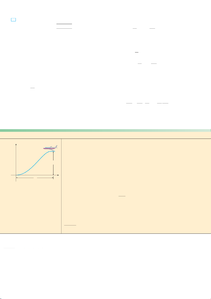
v EXAMPLE 4Find the points on the curve y 苷 x4 6x 2 w 4 here the tangent line is (0, 4) horizontal.
SOLUTION Horizontal tangents occur where the derivative is zero. We have 0 x dy 苷 d d d x 4 6 x 2 4 dx dx dx dx {_ œ „3, _5} {œ„3, _5} 苷 4x3 12x 0 苷 4x x 2 3 FIGURE 3 Thus dy dx 苷 i
0f x 苷 0 or x 2 3 苷 , 0 that is, x 苷 s . 3 So the given curve has y=x$-6x@+4
horizontal tangents when x The curve and
苷 0, s3 , and s3 . The corresponding points are 0, 4 , its horizontal tangents
(s3 , 5 ), and ( s3 , 5 ). (See Figure 3.)
EXAMPLE 5The equation of motion of a particle is s 苷 2t3 5t 2 3t , w 4 here is
measured in centimeters and t in seconds. Find the acceleration as a function of time.
What is the acceleration after 2 seconds?
SOLUTION The velocity and acceleration are v t 苷 ds苷 6t2 10t 3 dt a t 苷 dv苷 12t 10 dt
The acceleration after 2 s is a 2 苷 14 cm . s2
Next we need a formula for the derivative of a product of two functions. By analogy
with the Sum and Difference Rules, one might be tempted to guess, as Leibniz did three
centuries ago, that the derivative of a product is the product of the derivatives. We can see,
however, that this guess is wrong by looking at a particular example. Let f x 苷an x d t x 苷 . xT 2 hen the Power Rule gives f x and 苷 1 t . x But 苷 2x , f t so x 苷 x3 | ft x . Th 苷 us 3 x 2 ft . The c
苷 ofrretct formula was discovered by Leibniz (soon
after his false start) and is called the Product Rule.
The Product Rule If f and t are both differentiable, then
We can write the Product Rule in prime notation as d d d f x t x 苷 f xt x t x f x ft 苷 ft t f dx dx dx DIFFERENTIATION FORMULAS 131
PROOF Let F x 苷 f x . tThe x n F x h F x F x 苷 lim h l 0 h 苷 f x h t x h f x t x lim h l 0 h
In order to evaluate this limit, we would like to separate the functions f and t as in
the proof of the Sum Rule. We can achieve this separation by subtracting and adding the term f x h t in x the numerator: f x h t x h f x h t x f x h t x f x t x F x 苷 lim h l 0 h 苷 f x h f x lim t x h t x f x h t x h h l 0 h 苷 t x h t x f x h f x limf x h ⴢ lim limt x ⴢ lim h l 0 h l 0 h h l 0 h l 0 h 苷 f x t x t x f x Note that lim t x 苷 t b x ecause t is
x a constant with respect to the variable . h l 0 h
Also, since f is differentiable at x, it is continuous at x by Theorem 2.2.4, and so lim
苷 f . (See Exercise 59 in Section 1.8.) h l 0 f x h x
In words, the Product Rule says that the derivative of a product of two functions is the
first function times the derivative of the second function plus the second function times the
derivative of the first function. EXAMPLE 6 Find F if x F x 苷 6x.3 7x 4
SOLUTION By the Product Rule, we have d d F x 苷 6x3 7x4 7x 4 6x 3 dx dx 苷 6x3 28x 3 7x 4 18x 2 苷 168x6
126x 6 苷 294x 6
Notice that we could verify the answer to Example 6 directly by first multiplying the factors: F x 苷 6x3 7x 4 苷 42x7 ? F x
苷 42 7x6 苷 294x6
But later we will meet functions, such as y 苷 x2 sin ,
x for which the Product Rule is the only possible method. 132 CHAPTER 2
v EXAMPLE 7If h共x兲 苷 axntd i 共 tx is 兲 known that tan 共d3 兲 苷 5 , fintd ⬘ 共3 . 兲 苷 2 h⬘共3兲
SOLUTION Applying the Product Rule, we get d h⬘共x兲 苷
d 关xt共x兲兴 苷 x
关t共x兲兴 ⫹ t共x兲 d 关x兴 dx dx dx
苷 xt⬘共x兲 ⫹ t共x兲 Therefore
h⬘共3兲 苷 3t⬘共3兲 ⫹ t共3兲 苷 3 ⴢ 2 ⫹ 5 苷 11
The Quotient Rule If f and t are differentiable, then
In prime notation we can write the Quotient Rule as
t共x兲 d关 f 共x兲兴 ⫺ f 共x 关 兲 d t共x兲兴
t f ⬘ ⫺ ft⬘ d 冉f 冊⬘ 苷 t t2 冋f共x兲 册dx dx 苷 dx t共x兲 关t共x兲兴2
PROOF Let F共x兲 苷 f 共x . T 兲 h 兾etn 共x兲
f 共x ⫹ h兲 f 共x兲
F共x ⫹ h兲 ⫺ F共x兲
t共x ⫹ h兲 ⫺t共x兲
F⬘共x兲 苷 lim 苷 lim h l 0 h h l 0 h 苷
f 共x ⫹ h兲 t共x兲 ⫺ f 共x兲 t共x ⫹ h兲 lim h l 0
h t共x ⫹ h兲 t共x兲
We can separate f and t in this expression by subtracting and adding the termf 共x兲t共x兲 in the numerator:
f 共x ⫹ h兲 t共x兲 ⫺ f 共x兲 t共x兲 ⫹ f 共x兲 t共x兲 ⫺ f 共x兲 t共x ⫹ h兲
F⬘共x兲 苷 lim h l 0
h t共x ⫹ h兲 t共x兲
共x ⫹ h兲 ⫺ 共x兲 h兲 t共x兲 t共x兲 f f
⫺ f 共x兲 t共x ⫹ ⫺ 苷 h h lim h l 0
t共x ⫹ h兲t共x兲
f 共x ⫹ h兲 ⫺ f 共x兲
t共x ⫹ h兲 ⫺ t共x兲 limt共x兲 ⴢ l im
⫺ limf 共x兲 ⴢ lim 苷 hl0 h l 0 h h l 0 h l 0 h
limt共x ⫹ h兲 ⴢ litm 共x兲 h l 0 h l 0
苷 t共x兲 f ⬘共x兲 ⫺ f 共x兲t⬘共x兲 关t共x兲兴2
Again t is continuous by Theorem 2.2.4, so lim
t共x ⫹ h兲 苷 t . 共 h l 0 x兲
In words, the Quotient Rule says that the derivative of a quotient is the denominator
times the derivative of the numerator minus the numerator times the derivative of the
denominator, all divided by the square of the denominator.
The theorems of this section show that any polynomial is differentiable on ⺢ and any
rational function is differentiable on its domain. Furthermore, the Quotient Rule and the DIFFERENTIATION FORMULAS 133
other differentiation formulas enable us to compute the derivative of any rational func-
tion, as the next example illustrates.
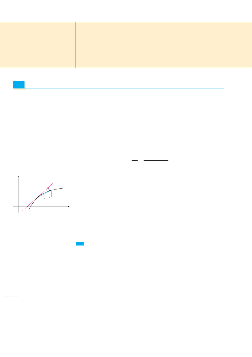
We can use a graphing device to check that
v EXAMPLE 8Let y 苷 x2 ⫹ x ⫺ 2 . Then x 3 ⫹ 6
the answer to Example 8 is plausible. Figure 4
shows the graphs of the function of Example 8 d d
and its derivative. Notice that when y grows x 3 ⫹ 6 x 2 ⫹ x ⫺ 2 ⫺ x 2 ⫹ x ⫺ 2 x 3 ⫹ 6 rapidly (near ⫺2),
y⬘ is large. And when y dx dx y⬘ 苷 grows slowly, y is ⬘ near . 0 x 3 ⫹ 6 2 1.5 苷 x3 ⫹ 6 2x ⫹ 1 ⫺ x 2 ⫹ x ⫺ 2 3x 2 x 3 ⫹ 6 2 yª
苷 2x4 ⫹ x3 ⫹ 12x ⫹ 6 ⫺ 3x4 ⫹ 3x3 ⫺ 6x2 _4 4 x 3 ⫹ 6 2 y
苷 ⫺x4 ⫺ 2x3 ⫹ 6x2 ⫹ 12x ⫹ 6 x 3 ⫹ 6 2 _1.5 FIGURE 4
NOTE Don’t use the Quotient Rule every time you see a quotient. Sometimes it’s eas-
ier to rewrite a quotient first to put it in a form that is simpler for the purpose of differenti-
ation. For instance, although it is possible to differentiate the function F x 苷 3x 2 ⫹ 2 sx x
using the Quotient Rule, it is much easier to perform the division first and write the func- tion as F x
苷 3x ⫹ 2x⫺1 2 before differentiating. General Power Functions
The Quotient Rule can be used to extend the Power Rule to the case where the exponent is a negative integer.
If n is a positive integer, then d x⫺n 苷 ⫺nx⫺ ⫺ n 1 dx d PROOF 1 x ⫺n 苷d dx dx x n d d x n 1 ⫺ 1 ⴢ x n 苷 dx dx
苷 xn ⴢ 0 ⫺ 1 ⴢ nxn⫺1 x n 2 x 2n
苷 ⫺nxn⫺1 苷 ⫺nxn⫺1⫺2n 苷 ⫺nx⫺n⫺1 x 2n 134 CHAPTER 2 EXAMPLE 9 dy 1 (a) If y 苷 1 , then 苷 d x ⫺1 苷 ⫺x⫺2 苷 ⫺ x dx dx x 2 d 18 (b) 6 苷 d 6 t ⫺3
苷 6 ⫺3 t⫺4 苷 ⫺ dt t 3 dt t 4
So far we know that the Power Rule holds if the exponent n is a positive or negative integer. If n 苷 , 0 then x 0 苷 ,
1 which we know has a derivative of 0. Thus the Power Rule
holds for any integer n . What if the exponent is a fraction? In Example 3 in Section 2.2 we found that d sx 苷 1 dx 2 sx which can be written as d x1 2 苷 1 x⫺1 2 dx 2
This shows that the Power Rule is true even when n 苷 .
1 In fact, it also holds for any real 2
number n, as we will prove in Chapter 6. (A proof for rational values of n is indicated in
Exercise 48 in Section 2.6.) In the meantime we state the general version and use it in the examples and exercises.
The Power Rule (General Version) If n is any real number, then d x n 苷 nxn⫺1 dx EXAMPLE 10 (a) If f x
苷 , xthen f ⬘ x 苷x ⫺ .1 (b) Let y 苷 1 s3 x2 dy Then 苷 d x⫺2 3 苷 ⫺2 x⫺ 2 3 ⫺1 dx dx 3 苷 ⫺2x⫺5 3 3 In Example 11, a and b are constants. It is
EXAMPLE 11Differentiate the function f t 苷 st a ⫹ .bt
customary in mathematics to use letters near theSOLUTION 1 Using the Product Rule, we have
beginning of the alphabet to represent constants
and letters near the end of the alphabet to repre- sent variables. d d f ⬘ t 苷 st a ⫹ bt ⫹
a ⫹ bt (st ) dt dt
苷 st ⴢ b ⫹ a ⫹ bt ⴢ 1 t ⫺1 2 2 苷 a ⫹ bt bst ⫹ 苷 a ⫹ 3bt 2 st 2 st DIFFERENTIATION FORMULAS 135
SOLUTION 2 If we first use the laws of exponents to rewritef t , then we can proceed
directly without using the Product Rule. f t
苷 ast ⫹ btst 苷 at1 2 ⫹ bt3 2 f ⬘ t 苷 1 at⫺1 2 ⫹ 3 2 bt1 2 2
which is equivalent to the answer given in Solution 1.
The differentiation rules enable us to find tangent lines without having to resort to the
definition of a derivative. They also enable us to find normal lines. The normal line to a
curve C at point P is the line through P that is perpendicular to the tangent line at P. (In
the study of optics, one needs to consider the angle between a light ray and the normal line to a lens.)
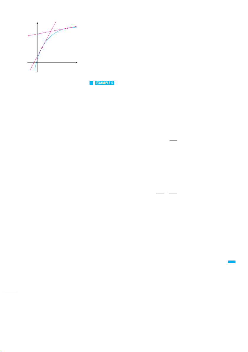
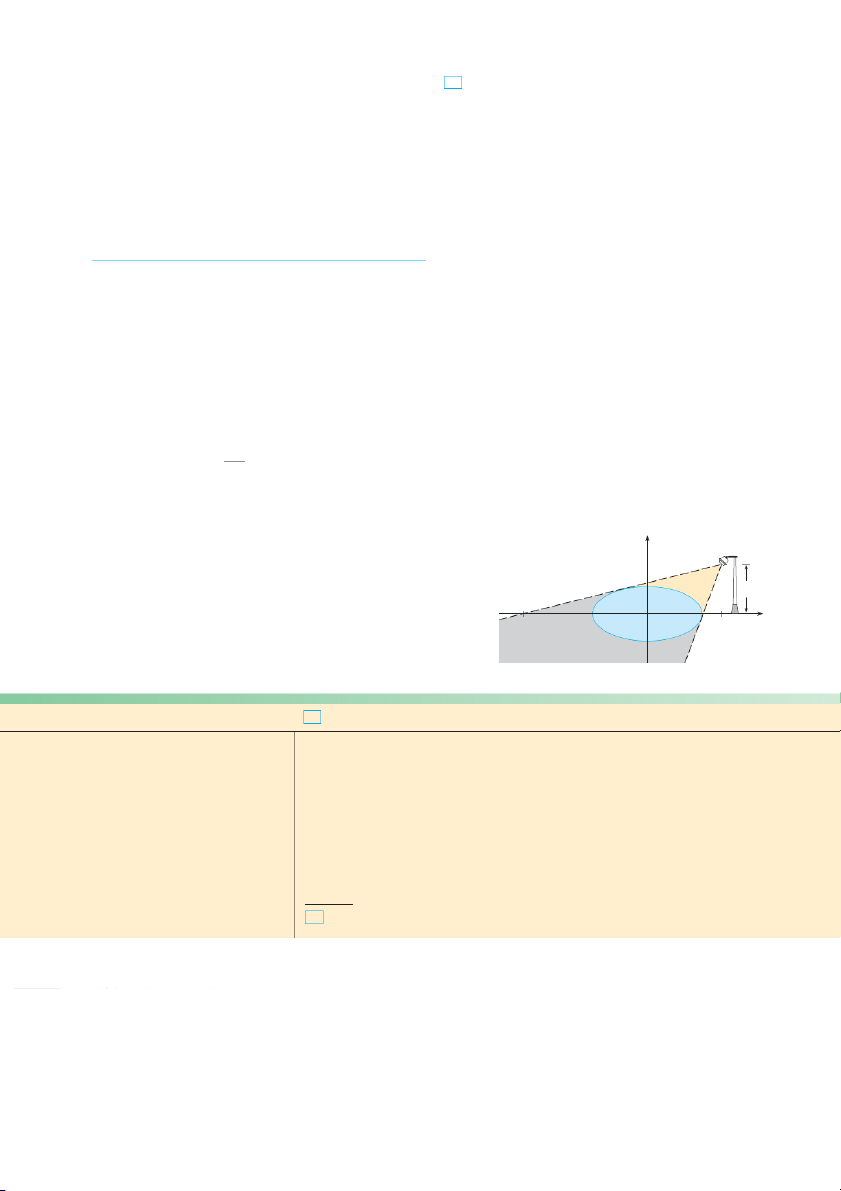
EXAMPLE 12Find equations of the tangent line and normal line to the curve y 苷 sx
1 ⫹ x 2 at the point (1, 1 .) 2
SOLUTION According to the Quotient Rule, we have d d 1 ⫹ x 2 (sx ) ⫺ sx 1 ⫹ x 2 dy 苷 dx dx dx 1 ⫹ x 2 2 1 1 ⫹ x 2 ⫺ sx 2x 苷 2 sx 1 ⫹ x 2 2
苷 1 ⫹ x2 ⫺ 4x2苷 1 ⫺ 3x 2 2 sx 1 ⫹ x 2 2 2 sx 1 ⫹ x 2 2
So the slope of the tangent line at (1, 1 ) is 2 dy ⴢ 1 苷 1 ⫺ 3 12 苷 ⫺ dx x苷1 2 s1 1 ⫹ 12 2 4 y normal
We use the point-slope form to write an equation of the tangent line at (1, 1): 2 1 tangent
y ⫺ 1 苷 ⫺ 1 x ⫺ 1 or y 苷 ⫺1 x ⫹ 3 2 4 4 4
The slope of the normal line at (1, 1 ) is the negative reciprocal of ⫺1, namely 4, so an 2 4 equation is 0 x 2
y ⫺ 1 苷 4 x ⫺ 1 or y 苷 4x ⫺ 7 2 2 FIGURE 5
The curve and its tangent and normal lines are graphed in Figure 5.
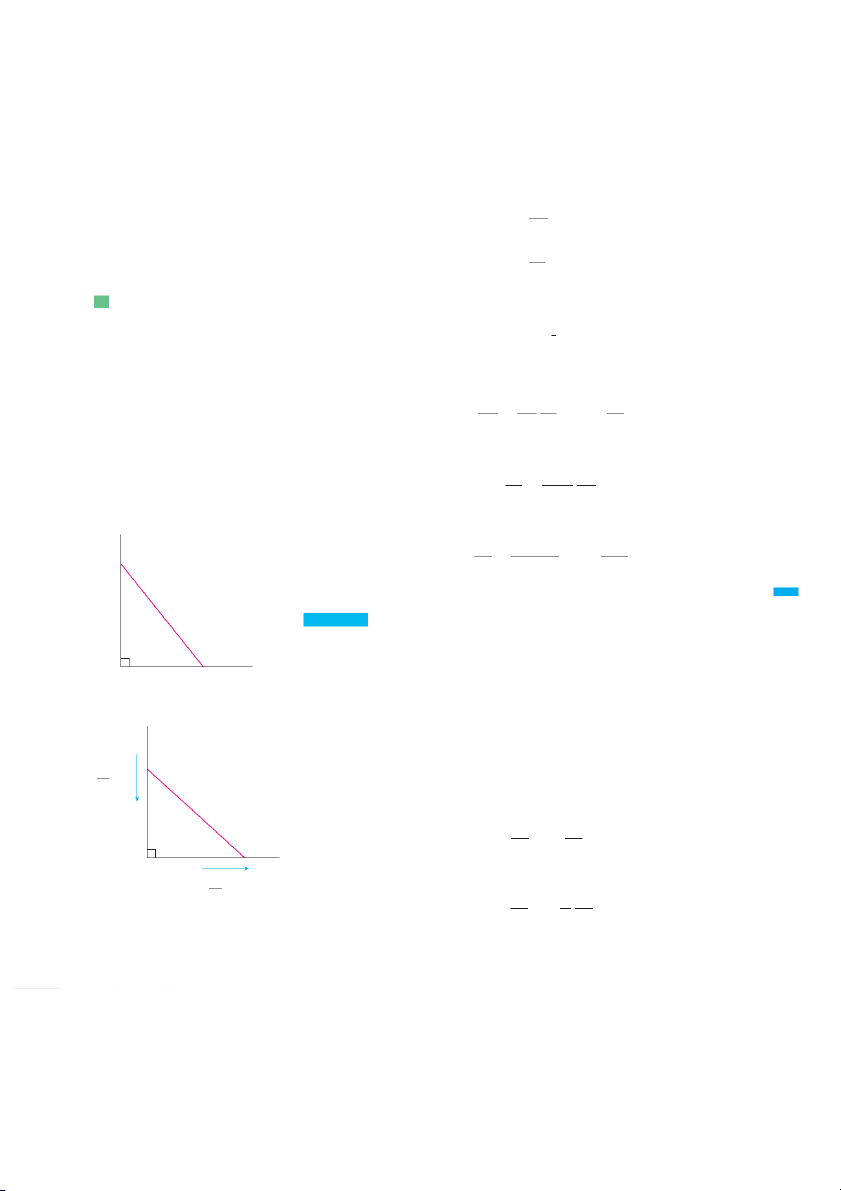
EXAMPLE 13At what points on the hyperbola xy 苷 12 is the tangent line parallel to the
line 3x ⫹ y 苷 ? 0
SOLUTION Sincex y 苷 12 can be written as y 苷 12 x , we have dy 苷 d 12 12 x ⫺1 苷 12 ⫺x⫺2 苷 ⫺ dx dx x 2 136 CHAPTER 2 y
Let the x-coordinate of one of the points in question be a. Then the slope of the tangent
line at that point is ⫺12 a .2 This tangent line will be parallel to the line 3x ⫹ y 苷 , 0 or (2, 6)xy=12 y 苷 ⫺3 ,
x if it has the same slope, that is, ⫺ . 3 Equating slopes, we get 12 ⫺ 苷 ⫺3 or a 2 苷 4 or a 苷 ⫾2 a 2 0 x
Therefore the required points are 2, 6 and ⫺ . ⫺ 2, T
6 he hyperbola and the tangents (_2, _6) are shown in Figure 6. 3x+y=0
We summarize the differentiation formulas we have learned so far as follows. FIGURE 6 d d
Table of Differentiation Formulas c 苷 0 x n 苷 nxn⫺1 dx dx cf ⬘ 苷 cf⬘
f ⫹ t ⬘ 苷 f ⬘ ⫹ t⬘
f ⫺ t ⬘ 苷 f ⬘ ⫺ t⬘
⬘tf⬘ ⫺ ft⬘
ft ⬘ 苷 ft⬘ ⫹ tf ⬘ f 苷 t t2 2.3 Exercises
1–22 Differentiate the function.
23. Find the derivative of f x 苷 1 ⫹ 2x2 x i ⫺ nx t2wo ways: 1. f x 苷 240 2. f x 苷 2
by using the Product Rule and by performing the multiplication first. Do your answers agree? 3. f t 苷 2 ⫺ 2 3 t 4. F x 苷 3 x 8 4
24. Find the derivative of the function 5. f x
苷 x3 ⫺ 4x ⫹ 6 6. f t 苷 1
t 6 ⫺ 3t 4 ⫹ t 2
x 4 ⫺ 5x 3 ⫹ sx F x 苷 7. t x 苷 x2 1 ⫺ 2x 8. h x 苷 x ⫺ 2 2x ⫹ 3 x 2 9. t t 苷 2t⫺3 4 10. B y 苷 cy⫺6
in two ways: by using the Quotient Rule and by simplifying
first. Show that your answers are equivalent. Which method do 12 you prefer? 11. A s 苷 ⫺
12. y 苷 x5 3 ⫺ x2 3 s 5 25– 44 Differentiate. 13. S p 苷 sp ⫺ p 14. y 苷 sx x ⫺ 1
25. V x 苷 2x3 ⫹ 3 x4 ⫺ 2x
15. R a 苷 3a ⫹ 1 2 16. S R 苷 R 2 4
26. L x 苷 1 ⫹ x ⫹ x2 2 ⫺ x 4 sx ⫹ x
17. y 苷 x2 ⫹ 4x ⫹ 3 18.y 苷 s 3 x x 2 27. F y 苷 1 ⫺ y ⫹ 5y3 y2 y4 19. H x
苷 x ⫹ x⫺1 3 20.
t u 苷 s2 u ⫹ s3u 28. J v 苷 v3 ⫺ 2v v⫺4 ⫹ v⫺2 2 21. u 苷 s 1 5 22. t ⫹ 4 st 5 v 苷 sx ⫹ s3 x 29. t x 苷1 ⫹ 2x 30.f x 苷x ⫺ 3 3 ⫺ 4x x ⫹ 3
; Graphing calculator or computer required
1. Homework Hints available at stewartcalculus.com DIFFERENTIATION FORMULAS 137
51–52 Find an equation of the tangent line to the curve at the 31. y 苷 x 3 32. y 苷 x 1 1 x 2 x 3 x 2 given point. v3 v 2 sv 51. y 苷 2x, 1, 1 33. y 苷 34. y 苷 t x 1 v t 1 2 52. y 苷 x 4 2x 2 , x 1, 2 35. y 苷 t 2 2 36. t t 苷 t st t 4 3t 2 1 t 1 3 B C 2 37.
53. (a) The curve y 苷 1 1
x is called a witch of Maria y 苷 ax2 bx c 38. y 苷 A x x 2
Agnesi. Find an equation of the tangent line to this curve at the point ( 1, 1 ) 2 . 39. f t 苷 2t 40. y 苷 cx ;
(b) Illustrate part (a) by graphing the curve and the tangent 2 st 1 cx line on the same screen. 2 41.
54. (a) The curve y 苷 x 1
x is called a serpentine. y 苷 s3 t t 2 t t 1 42. y 苷 u6 2u3 5 u2
Find an equation of the tangent line to this curve at the point . 3, 0.3 ;
(b) Illustrate part (a) by graphing the curve and the tangent 43. f x 苷 x 44. f x 苷 ax b c cx d line on the same screen. x x
55–58 Find equations of the tangent line and normal line to the curve at the given point.
45. The general polynomial of degree h n as the form 55. y 苷 x , sx 56. y 苷 1 , 2 x 2 1, 2 1, 9 P x 苷 an xn an 1 x n 1 a2 x 2 a1 x a0 where a 苷 n .
0 Find the derivative of P. 57. y 苷 3x 1 , 1, 2 58. y 苷 sx, 4, 0.4 x 2 1 x 1 ; 46–48 Find f . Co xmpare the graphs of an
f d f and use them
to explain why your answer is reasonable.
59–62 Find the first and second derivatives of the function. 46. f x 苷 x x 2 1 1 59. f x 苷 x4 3x 3 16x 60. G r 苷 sr 3sr 47. f x 苷 3x15 5x 3 3 48. f x 苷 x x 61. f x 苷 x 2 62. f x 苷 1 1 2x 3 x
; 49. (a) Use a graphing calculator or computer to graph the func- tion f x 苷 x4 3x 3 6x 2 7x in 30 the viewing rectangle by 3, 5 . 10, 50
63. The equation of motion of a particle is s 苷 t 3 3,t where s
(b) Using the graph in part (a) to estimate slopes, make
is in meters and t is in seconds. Find
a rough sketch, by hand, of the graph of f . (See
(a) the velocity and acceleration as functions of , t Example 1 in Section 2.2.)
(b) the acceleration after 2 s, and (c) Calculate f a
x nd use this expression, with a graphing
(c) the acceleration when the velocity is 0.
device, to graph f . Compare with your sketch in part (b).
64. The equation of motion of a particle is
; 50. (a) Use a graphing calculator or computer to graph the func- tion t x 苷 x2x2 i 1 n the viewing rectangle 4, 4 s 苷 t 4 2t 3 t 2 t by . 1, 1.5
(b) Using the graph in part (a) to estimate slopes, make a
where s is in meters and t is in seconds.
rough sketch, by hand, of the graph of t . (See Example 1
(a) Find the velocity and acceleration as functions of .t in Section 2.2.)
(b) Find the acceleration after 1 s. (c) Calculate t a
x nd use this expression, with a graphing ;
(c) Graph the position, velocity, and acceleration functions
device, to graph t . Compare with your sketch in part (b). on the same screen. 138 CHAPTER 2
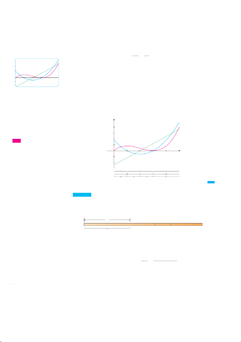
65. Boyle’s Law states that when a sample of gas is compressed 72. Let P x 苷 an F d Q x x G 苷 x F x , w
G hexre F and G
at a constant pressure, the pressure P of the gas is inversely
are the functions whose graphs are shown.
proportional to the volume V of the gas. (a) Find P . 2 (b) Find Q .7
(a) Suppose that the pressure of a sample of air that occupies y 0.106 m a 3 t 25 i Cs 50 kP .
a Write V as a function of . P (b) Calculate dV w
dP hen P 苷 50 kP . a What is the meaning F
of the derivative? What are its units?
; 66. Car tires need to be inflated properly because overinflation or G 1
underinflation can cause premature treadware. The data in the
table show tire life L ( in thousands of miles) for a certain 0 x 1
type of tire at various pressures ( in lb in )2 P .
73. If t is a differentiable function, find an expression for the P 26 28 31 35 38 42 45
derivative of each of the following functions. t x L 50 66 78 81 74 70 59
(a) y 苷 xt x (b) y 苷 x (c) y 苷 t x x
74. If f is a differentiable function, find an expression for the
(a) Use a graphing calculator or computer to model tire life
derivative of each of the following functions.
with a quadratic function of the pressure.
(b) Use the model to estimate dL w
dP hen P 苷 30 and when
(a) y 苷 x 2 f x (b) y 苷 f x P 苷 .
40 What is the meaning of the derivative? What are x 2
the units? What is the significance of the signs of the derivatives? (c) y 苷 x 2 (d) y 苷 1 x f x f x sx 67. Suppose that ,f 5 f苷 , 1 5 t苷56 , 苷 and3 t 5 . 苷 2
75. Find the points on the curvey 苷 2x 3 3x 2 12x 1 Find the following values.
where the tangent is horizontal. (a) ft 5 (b) f t 5
76. For what values of x does the graph of (c) t f 5 f x 苷 x3 3x 2 x ha 3 ve a horizontal tangent?
77. Show that the curve y 苷 6x 3 5x 3 has no tangent line 68. Find , giv hen tha 2 t f 2 , 苷 t 2 3 , f苷 4 2 苷 , 2 with slope 4. and t 2 . 苷 7 (a) h x 苷 5f x ( 4 bt) h x x 苷 f x t x
78. Find an equation of the tangent line to the curve y 苷 x sx t x
that is parallel to the line y 苷 1 3 . x (c) h x 苷f x (d) h x 苷 t x 1 f x
79. Find equations of both lines that are tangent to the curve y 苷 1 x a
3 nd are parallel to the line 12x y 苷 .1 69. If f x , w 苷 hsexret x t a 4 nd 苷 t 8 4 , fin 苷d f7 . 4
80. Find equations of the tangent lines to the curve 70. If h 2 and 苷 h4 2 苷 , fin 3 d y 苷 x 1 x 1 d h x
that are parallel to the line x y 2 苷 .2 dx x x苷2
81. Find an equation of the normal line to the parabola
71. If f and t are the functions whose graphs are shown, let y 苷 x 2 5x
4 that is parallel to the line x y 3 苷 . 5 u x 苷and f vx xt 苷 x f x . t x
82. Where does the normal line to the parabola y 苷 x x 2 at the (a) Find u 1 . (b) Find v 5 .
point (1, 0) intersect the parabola a second time? Illustrate with a sketch. y
83. Draw a diagram to show that there are two tangent lines to the parabola y 苷 th x a
2 t pass through the point 0, . 4 Find f
the coordinates of the points where these tangent lines inter- g sect the parabola. 1
84. (a) Find equations of both lines through the point 2, 3 0 x 1
that are tangent to the parabola y 苷 x 2 .x DIFFERENTIATION FORMULAS 139
(b) Show that there is no line through the point 2, 7 that is
94. At what numbers is the following functiont differentiable?
tangent to the parabola. Then draw a diagram to see why. 2x if x 0
85. (a) Use the Product Rule twice to prove that if f, ,t and hare t x 苷 2x x 2 if 0 x 2 differentiable, then fth 苷 f th ft h .fth 2 x if x 2
(b) Taking f 苷 t 苷 hin part (a), show that t t t d Give a formula for and sketch the graphs of and . f x 3 苷 3 f x 2 f x dx
95. (a) For what values of x is the function f x 苷x2 9
(c) Use part (b) to differentiate y 苷 x 4 3x 3 17x 82. 3
differentiable? Find a formula for f . (b) Sketch the graphs of a f nd f .
86. Find the nthderivative of each function by calculating the first
few derivatives and observing the pattern that occurs.
96. Where is the function h x 苷x 1 x 2 differenti - (a) h h h f x 苷 xn (b) f x 苷 1 x able? Give a formula for and sketch the graphs of and .
87. Find a second-degree polynomial suc 97. P h that P 2 , 苷 5
For what values of aand b is the line 2x
y 苷 b tangent to y 苷 ax2 x 苷 2 P , 2 and 苷P3 2 . 苷 2 the parabola when ? 苷 88. F x f x t x f t The equation y y 2y 苷 is
x 2called a differential 98. (a) If
, where and have derivatives of all F 苷 f t 2 f t f t
equation because it involves an unknown function y and its orders, show that . 4
derivatives yand y . Find constants A B , , and C such that the
(b) Find similar formulas for F and F . n
function y 苷 Ax 2 Bx
C satisfies this equation. (Differen-
(c) Guess a formula for F .
tial equations will be studied in detail in Chapter 9.)
99. Find the value of c such that the line y 苷 32x 6 is tangent to
89. Find a cubic function y 苷 ax3 bx 2 cx d whose graph
the curve y 苷 csx .
has horizontal tangents at the points an 2, 6 d . 2, 0 100. Let
90. Find a parabola with equation y 苷 ax2 bx cthat has if x 2 slope 4 at x 苷 , 1 slope 8 at x 苷 , 1 and passes through the f x 苷 x 2 mx b if x 2 point . 2, 15 m b f 91. Find the values of and that make differentiable
In this exercise we estimate the rate at which the total personal everywhere.
income is rising in the Richmond-Petersburg, Virginia, metro-
politan area. In 1999, the population of this area was 961,400,
101. An easy proof of the Quotient Rule can be given if we make
and the population was increasing at roughly 9200 people per
the prior assumption that F ex
x ists, where F 苷 f . tWrite
year. The average annual income was $30,593 per capita, and
f 苷 Ft ; then differentiate using the Product Rule and solve the
this average was increasing at about $1400 per year (a little
resulting equation for F.
above the national average of about $1225 yearly). Use the
Product Rule and these figures to estimate the rate at which
102. A tangent line is drawn to the hyperbola xy 苷 cat a point . P
total personal income was rising in the Richmond-Petersburg
(a) Show that the midpoint of the line segment cut from this
area in 1999. Explain the meaning of each term in the Product
tangent line by the coordinate axes is P. Rule.
(b) Show that the triangle formed by the tangent line and the
coordinate axes always has the same area, no matter where
92. A manufacturer produces bolts of a fabric with a fixed width.
P is located on the hyperbola.
The quantity q of this fabric (measured in yards) that is sold is
a function of the selling price p ( in dollars per yard), so we can x 1000 1 write q 苷 f .
p Then the total revenue earned with selling 103. Evaluate lim . x l 1 x 1 price p is R p 苷 pf . p
(a) What does it mean to say that f 20 苷 and 10,000
104. Draw a diagram showing two perpendicular lines that intersect f 20 苷 ?350 on the -
y axis and are both tangent to the parabola y 苷 x .2
(b) Assuming the values in part (a), find R a 20 nd interpret
Where do these lines intersect? your answer. 105. If c ,
1 how many lines through the point 0, care normal 2 93. Let
lines to the parabola y 苷 x ? 2 What if c ? 1 2 if x 1 f x 苷 x 2 1
106. Sketch the parabolas y 苷 x2and y 苷 x2 2x . 2 Do you x 1 if x 1
think there is a line that is tangent to both curves? If so, find its Is d
f ifferentiable at 1? Sketch the graphs of a f nd f . equation. If not, why not? 140 CHAPTER 2 A P P L I E D P R O J E C T
BUILDING A BETTER ROLLER COASTER
Suppose you are asked to design the first ascent and drop for a new roller coaster. By studying
photographs of your favorite coasters, you decide to make the slope of the ascent 0.8 and the slope
of the drop 1.6. You decide to connect these two straight stretches y 苷 L 共 兲 共 1 a x nd y 苷 L w 2 ith x兲 f
part of a parabola y 苷 f 共x兲 苷 a x 2 bx , wh c ere and x f are 共 xme
兲 asured in feet. For the track L¡ P
to be smooth there can’t be abrupt changes in direction, so you want the linear segments L1 and L 2
to be tangent to the parabola at the transition points P and Q . (See the figure.) To simplify the
equations, you decide to place the origin at P. Q L™
1. (a) Suppose the horizontal distance between P and Q is 100 ft. Write equations in a, b,
and c that will ensure that the track is smooth at the transition points.
(b) Solve the equations in part (a) for a b
, , and c to find a formula for f 共 .x兲 ; (c) Plot , L1 , a f nd t L o
2 verify graphically that the transitions are smooth.
(d) Find the difference in elevation between P and . Q
2. The solution in Problem 1 might look smooth, but it might not feel smooth because the
piecewise defined function [consisting of L 共x兲 x 0 f 共 1 for , for x兲 0 x , and 100 L 共 兲 2 f x or x ] do
100 esn’t have a continuous second derivative. So you decide to improve
the design by using a quadratic function q共x兲 苷 ax2 bx onl c y on the interval 10 x
90 and connecting it to the linear functions by means of two cubic functions: t共x兲 苷 kx3 lx2 m x n 0 x 10
h共x兲 苷 px3 qx 2 rx s 90 x 100
(a) Write a system of equations in 11 unknowns that ensure that the functions and their
first two derivatives agree at the transition points. CAS
(b) Solve the equations in part (a) with a computer algebra system to find formulas for
q共x兲, t共x兲, a . nd h共x兲 (c) Plot L , t
1 , q , h , and L 2, and compare with the plot in Problem 1(c).
© Flashon Studio / Shutterstock
; Graphing calculator or computer required
CAS Computer algebra system required 2.4
Derivatives of Trigonometric Functions
A review of trigonometric functions is given in Before starting this section, you might need to review the trigonometric functions. In par- Appendix D.
ticular, it is important to remember that when we talk about the function f defined for all real numbers x by
f 共x兲 苷 sin x
it is understood that sin x means the sine of the angle whose radian measure is x. A simi-
lar convention holds for the other trigonometric functions cos, tan, csc, sec, and cot. Recall
from Section 1.8 that all of the trigonometric functions are continuous at every number in their domains.
If we sketch the graph of the function f 共x兲 an
苷 d siuns ex the interpretation of f 共x兲
as the slope of the tangent to the sine curve in order to sketch the graph of f (see Exer-
cise 16 in Section 2.2), then it looks as if the graph of f may be the same as the cosine curve (see Figure 1).
DERIVATIVES OF TRIGONOMETRIC FUNCTIONS 1 y y= ƒ=sin x 0 π x π 2π 2
TEC Visual 2.4 shows an animation of Figure 1. y y= fª(x) 0 π x π 2 FIGURE 1
Let’s try to confirm our guess that if f x 苷 si ,n th x en f x . 苷 Fcroosm x the defini- tion of a derivative, we have f x h f x sin x h sin x f x 苷 lim 苷 lim h l 0 h h l 0 h
We have used the addition formula for sine. 苷 sin x cos h cos x sin h sin x lim See Appendix D. h l 0 h 苷 cos x sin h lim sin x cos h sin x h l 0 h h 苷 lim cos h 1 sin h sin x cos x h l 0 h h cos h 1 sin h 1 苷 limsin x ⴢ lim limcos x ⴢ lim h l 0 h l 0 h h l 0 h l 0 h
Two of these four limits are easy to evaluate. Since we regard x as a constant when com-
puting a limit as h l 0 , we have
limsin x 苷 sin x and
lim cos x 苷 cos x h l 0 h l 0 The limit of sin h is
h not so obvious. In Example 3 in Section 1.5 we made the guess,
on the basis of numerical and graphical evidence, that sin 2 lim 苷 1 l 0
We now use a geometric argument to prove Equation 2. Assume first that lies between 0 and .
2 Figure 2(a) shows a sector of a circle with center O, central angle , and 142 CHAPTER 2 D
radius 1. BC is drawn perpendicular to OA. By the definition of radian measure, we have arc AB 苷 . Also . From the diagram we see that
ⱍBCⱍ苷ⱍOBⱍsin 苷 sin B
ⱍBC ⱍ⬍ ⱍABⱍ⬍ arc AB 1 E Therefore sin ⬍ sin so ⬍ 1 ¨
Let the tangent lines at A and B intersect at E . You can see from Figure 2(b) that the O
cir cumference of a circle is smaller than the length of a circumscribed polygon, and so C A arc AB ⬍ . Thus (a)
ⱍAEⱍ⫹ ⱍEBⱍ 苷 arc AB ⬍ B
ⱍAEⱍ⫹ ⱍEBⱍ E
⬍ ⱍAEⱍ⫹ ⱍEDⱍ O A
苷 ⱍADⱍ苷 ⱍOAⱍtan 苷 tan
(In Appendix F the inequality 艋 tan is proved directly from the definition of the length (b)
of an arc without resorting to geometric intuition as we did here.) Therefore we have FIGURE 2 ⬍ sin cos so cos ⬍ sin ⬍ 1
We know that lim l 0 1 苷 1 and lim l0 cos
苷 ,1 so by the Squeeze Theorem, we have sin lim 苷 1 l0⫹ But the function 共sin 兲 is
兾 an even function, so its right and left limits must be equal. Hence, we have sin lim 苷 1 l 0 so we have proved Equation 2.
We can deduce the value of the remaining limit in 1 as follows:
We multiply numerator and denominator by cos ⫺ 1
cos ⫹ 1 in order to put the function in a form
in which we can use the limits we know. 冉 冊 cos2 ⫺1 lim 苷 lim cos ⫺ 1 ⴢ cos ⫹ 1 苷 lim l 0 l l 0 共 0 cos ⫹ 1 cos ⫹ 1兲 苷 ⫺sin2 冉 冊 lim 苷 ⫺lim sin ⴢ sin l 0 共cos ⫹ 1兲 l 0 cos ⫹ 1 苷 sin sin ⫺lim ⴢ lim l 0 l 0 cos ⫹ 1 冉 0冊 (by Equation 2) 苷 ⫺1 ⴢ 苷 0 1 ⫹ 1
DERIVATIVES OF TRIGONOMETRIC FUNCTIONS 1 cos 1 3 lim 苷 0 l 0
If we now put the limits 2 and 3 in 1 , we get cos h 1 sin h f x 苷 lsim n x ⴢ lim limcos x ⴢ lim h l 0 h l 0 h h l 0 h l 0 h 苷 sin x ⴢ 0 cos x ⴢ 1 苷 cos x
So we have proved the formula for the derivative of the sine function: d 4 sin x 苷 cos x dx
v EXAMPLE 1Differentiate y 苷 x2 sin .x
Figure 3 shows the graphs of the function of
SOLUTION Using the Product Rule and Formula 4, we have
Example 1 and its deriva tive. Notice that y whenever 苷 0 has y a horizontal tangent. dy 苷 d d x 2 sin x sin x x 2 dx dx dx 5 苷 x2 cos x 2x sin x yª y
Using the same methods as in the proof of Formula 4, one can prove (see Exercise 20) _4 4 that d 5 _5 cos x 苷 sin x dx FIGURE 3
The tangent function can also be differentiated by using the definition of a derivative,
but it is easier to use the Quotient Rule together with Formulas 4 and 5: d sin x tan x 苷d dx dx cos x d d cos x sin x sin x cos x 苷 dx dx cos2x
苷 cos x ⴢ cos x sin x sin x cos2x 苷 cos2x sin2x cos2x 苷 1 苷 sec2x cos2x 144 CHAPTER 2
d 共tan x兲 苷 sec2 6 x dx
The derivatives of the remaining trigonometric functions, csc , sec , and cot , can also be
found easily using the Quotient Rule (see Exercises 17–19). We collect all the differentia-
tion formulas for trigonometric functions in the following table. Remember that they are
valid only when x is measured in radians.
Derivatives of Trigonometric Functions d d
共sin x兲 苷 cos x
共csc x兲 苷 csc x cot x
When you memorize this table, it is helpful dx dx
to notice that the minus signs go with the der- d d
ivatives of the “cofunctions,” that is, cosine,
共cos x兲 苷 sin x
共sec x兲 苷 sec x tan x cosecant, and cotangent. dx dx d d
共tan x兲 苷 sec x 2
共cot x兲 苷 csc2x dx dx sec x
EXAMPLE 2Differentiate f 共x兲 苷
. For what values of x does the graph of f 1 tan x have a horizontal tangent?
SOLUTION The Quotient Rule gives 共 d 1 tan x兲 d 共sec x兲 sec x 共1 tan x兲 dx dx f 共x兲 苷 共1 tan x兲2 共 苷 1
tan x兲 sec x tan x sec x ⴢ sec2x 共1 tan x兲2 3
苷 sec x 共tan x tan2x sec2x兲 共1 tan x兲2 _3 5
苷 sec x 共tan x 1兲 共1 tan x兲2 _3
In simplifying the answer we have used the identity tan2x 1 苷 sec2 . x FIGURE 4 Since isse n c e
x ver 0, we see that f 共x兲 wh 苷 en 0 tan x 苷 , 1 and this occurs when
The horizontal tangents in Example 2 x 苷 n , 兾 w
4 here n is an integer (see Figure 4).
Trigonometric functions are often used in modeling real-world phenomena. In particu-
lar, vibrations, waves, elastic motions, and other quantities that vary in a periodic manner
can be described using trigonometric functions. In the following example we discuss an
instance of simple harmonic motion.
DERIVATIVES OF TRIGONOMETRIC FUNCTIONS 1
v EXAMPLE 3An object at the end of a vertical spring is stretched 4 cm beyond its rest
position and released at time t 苷 .
0 (See Figure 5 and note that the downward direction is
positive.) Its position at time t is 0 s 苷 f t 苷 4 cos t 4
Find the velocity and acceleration at time t and use them to analyze the motion of the s object. FIGURE 5
SOLUTION The velocity and acceleration are v 苷 ds 苷 d 4 cos t 苷 d 4 cos t 苷 4 sin t dt dt dt √ s a d
a 苷 dv 苷 d 4 sin t
苷 4 sin t 苷 4 cos t dt dt 2 dt
The object oscillates from the lowest point s 苷 4 cmto the highest point 0 π 2π t s 苷 4 c .
m The period of the oscillation is 2 , the period of cos t. _2
The speed is v 苷 4 sin t , which is greatest when sin t 苷 , 1 that is, when cos t 苷 .
0 So the object moves fastest as it passes through its equilibrium position s 苷 . I
0 ts speed is 0 when sin t 苷 ,
0 that is, at the high and low points. The acceleration a 苷
4 cos t 苷 0 when s 苷 .
0 It has greatest magnitude at the high FIGURE 6
and low points. See the graphs in Figure 6.
EXAMPLE 4 Find the 27th derivative of cos x.
SOLUTION The first few derivatives of f x 苷 cos axre as follows: PS Look for a pattern. f x 苷 sin x f x 苷 cos x f x 苷 sin x f 4 x 苷 cos x f 5 x 苷 sin x
We see that the successive derivatives occur in a cycle of length 4 and, in particular, f n x 苷 c w osh e
x never n is a multiple of 4. Therefore f 24 x 苷 cos x
and, differentiating three more times, we have f 27 x 苷 sin x
Our main use for the limit in Equation 2 has been to prove the differentiation formula
for the sine function. But this limit is also useful in finding certain other trigonometric lim-
its, as the following two examples show. sin 7x EXAMPLE 5 Find lim . x l 0 4x
SOLUTION In order to apply Equation 2, we first rewrite the function by multiplying and dividing by 7: sin 7x
Note that sin 7x 苷 7 sin . x 苷 7 sin 7x 4x 4 7x 146 CHAPTER 2 If we let 苷 7 , x then l 0
as x l 0 , so by Equation 2 we have sin 7x 冉 冊 lim 苷 7 lim sin 7x x l 0 4x 4 xl0 7x 苷 7 sin lim 苷 7 ⴢ 1 苷7 4 l0 4 4 v EXAMPLE 6Calculate lim x cot x . x l 0
SOLUTION Here we divide numerator and denominator by x : x cos x
limx cot x 苷 lim x l 0 x l 0 sin x limcos x 苷 cos x x l 0 lim 苷 x l 0 sin x sin x lim x x l 0 x 苷 cos 0
(by the continuity of cosine and Equation 2) 1 苷 1 2.4 Exercises 1–16 Differentiate.
20. Prove, using the definition of derivative, that if f 共x兲 苷 c , os x 1.
f 共x兲 苷 3x 2 ⫺ 2 cos x
2. f 共x兲 苷 sx sin x
then f ⬘共x兲 苷 ⫺ .sin x
3. f 共x兲 苷 sin x cot 21–24 2 ⫹ 1 x
4. y 苷 2 sec x ⫺ csc x
Find an equation of the tangent line to the curve at the given 5. point. y 苷 sec t an
6. t共t兲 苷 4 sec t ⫹ tan t 7.
21. y 苷 sec x, 共兾3, 2兲 22.
y 苷 共1 ⫹ x兲, c os x 共 兲 0, 1
y 苷 c cos t ⫹ t 2 sin t
8. y 苷 u共a cos u ⫹ b cot u兲
23. y 苷 cos x ⫺ sin x , 共, ⫺1兲
24. y 苷 x ⫹ tan , x 共 , 兲 9. y 苷 x 10. y 苷 sin cos 2 ⫺ tan x
25. (a) Find an equation of the tangent line to the curve 11. f 共兲 苷 sec 12. y 苷 cos x 1 ⫹ sec 1 ⫺ sin x y 苷 2x sin a
x t the point 共兾2, . 兲 ;
(b) Illustrate part (a) by graphing the curve and the tangent line 13. on the same screen.
y 苷 t sin t
14. y 苷 1 ⫺ sec x 1 ⫹ t tan x
26. (a) Find an equation of the tangent line to the curve
15. h共兲 苷 csc ⫺ cot
16. y 苷 x2 sin x tan x y 苷 x
3 ⫹ 6 cos x at the point 共兾3, ⫹ 3 . 兲 ;
(b) Illustrate part (a) by graphing the curve and the tangent line on the same screen. d 17. Prove that
共csc x兲 苷 ⫺csc x c .ot x dx
27. (a) If f 共x兲 苷 sec x , ⫺fin x d f .⬘共x兲 ;
(b) Check to see that your answer to part (a) is reasonable by d 18. ⬘ Prove that 共
graphing both f and f for . ⱍxⱍ ⬍ 兾 sec 2
x兲 苷 sec x t . an x dx
28. (a) If f 共x兲 苷 sx si , n fxind f . ⬘共x兲 d 19. ;
(b) Check to see that your answer to part (a) is reasonable by Prove that
共cot x兲 苷 ⫺c .sc2x dx
graphing both f and f f ⬘or 0 艋 x 艋 .2
; Graphing calculator or computer required
1. Homework Hints available at stewartcalculus.com
DERIVATIVES OF TRIGONOMETRIC FUNCTIONS 1
29. If H共兲 苷 sin , find H 共兲 and H .共 兲
38. An object with weight W is dragged along a horizontal plane
by a force acting along a rope attached to the object. If the
30. If f 共t兲 苷 , c f s in c d t f兾 . 共兲 6
rope makes an angle with the plane, then the magnitude of the force is
31. (a) Use the Quotient Rule to differentiate the function F 苷 W sin cos f 共x兲 苷 tan x 1 sec x where
is a constant called the coefficient of friction.
(a) Find the rate of change of F with respect to .
(b) Simplify the expression for f 共 b x y 兲writing it in terms
(b) When is this rate of change equal to 0? of sin x and cos ,
x and then find f . 共x兲 ; (c) If W 苷 lb 50 and 苷 , d 0.6raw the graph of as F a func-
(c) Show that your answers to parts (a) and (b) are
tion of and use it to locate the value of for which equivalent. dF兾d 苷 .
0 Is the value consistent with your answer to 32. Suppose part (b)? f 共兾3兲 a 苷 nd 4 f 共 兾3兲 苷 , an2d let
t共x兲 苷 f 共x a 兲 nsdi n x h共x兲 苷 . 共 F c i on s d
x兲兾f 共x兲 (a) t 共兾3兲 (b) 39–48 h 共 兾 兲 3 Find the limit. sin 3x sin 4x
33. For what values of x does the graph of f 共x兲 苷 x 2 sin x 39. lim 40. lim x l 0 x x l 0 sin 6x have a horizontal tangent? tan 6t cos 1
34. Find the points on the curve y 苷 共cos x兲兾共2 at s iw n h x ich 兲 41. lim 42. lim t l 0 sin 2t l 0 sin the tangent is horizontal. sin 3x sin 3x sin 5x
35. A mass on a spring vibrates horizontally on a smooth 43. lim 44. lim x l 0 5x 3 4x x l 0 x 2
level surface (see the figure). Its equation of motion is x共t兲 苷 8 , s iw n h
t ere is itn seconds and in c x entimeters. sin sin共x 2兲
(a) Find the velocity and acceleration at time .t 45. lim 46. lim l 0 tan x l 0 x
(b) Find the position, velocity, and acceleration of the mass at time t 苷 2 . 兾 I
3 n what direction is it moving at that 1 tan x sin共x 1兲 time? 47. lim 48. lim x l 兾4 sin x cos x x l 1 x 2 x 2 equilibrium position
49–50 Find the given derivative by finding the first few deriva-
tives and observing the pattern that occurs. d 99 49. 共sin x兲 d 35 50. 共 x x 0 x sin x兲 dx99 dx35
; 36. An elastic band is hung on a hook and a mass is hung on the
lower end of the band. When the mass is pulled downward
51. Find constants A and B such that the function
and then released, it vibrates vertically. The equation of
y 苷 A sin x
B cos x satisfies the differential equation
motion is s 苷 2 cos t 3 sin , t t , 0 where sis measured y y 2y 苷 si . n x
in centi meters and t in seconds. (Take the positive direction to be downward.) 1
(a) Find the velocity and acceleration at time .t
52. (a) Evaluate limx sin . x l x
(b) Graph the velocity and acceleration functions.
(c) When does the mass pass through the equilibrium 1 (b) Evaluate limx sin . position for the first time? x l 0 x
(d) How far from its equilibrium position does the mass ;
(c) Illustrate parts (a) and (b) by graphing y 苷 x sin共 .1兾x兲 travel?
(e) When is the speed the greatest?
53. Differentiate each trigonometric identity to obtain a new (or familiar) identity.
37. A ladder 10 ft long rests against a vertical wall. Let be the
angle between the top of the ladder and the wall and let x be
(a) tan x 苷 sin x (b) sec x 苷 1
the distance from the bottom of the ladder to the wall. If the cos x cos x
bottom of the ladder slides away from the wall, how fast does (c) sin x cos x 苷 1 cot x
x change with respect to when 苷 ? 兾3 csc x 148 CHAPTER 2
54. A semicircle with diameter PQ sits on an isosceles triangle
55. The figure shows a circular arc of length s and a chord of
PQR to form a region shaped like a two-dimensional ice-
length d , both subtended by a central angle . Find
cream cone, as shown in the figure. If A共 is 兲 the area of the s lim semicircle and B共 is
兲 the area of the triangle, find l 0 d A共兲 s lim d l 0 B共兲 ¨ A(¨) P Q B(¨)
; 56. Let f 共x兲 苷 x . s1 cos 2x 10 cm 10 cm
(a) Graph .f What type of discontinuity does it appear to ¨ have at 0?
(b) Calculate the left and right limits of f at 0. Do these R
values confirm your answer to part (a)? 2.5 The Chain Rule
Suppose you are asked to differentiate the function
F共x兲 苷 sx 2 1
The differentiation formulas you learned in the previous sections of this chapter do not
enable you to calculate F . 共x兲
See Section 1.3 for a review of composite
Observe that F is a composite function. In fact, if we let y 苷 f 共u兲 苷 a s n u d let functions.
u 苷 t共x兲 苷 x 2 , the 1 n we can write
y 苷 F共x兲 , 苷 tfhat 共 tis, 共 x兲兲 . We k Fnow 苷 f ⴰ t
how to differentiate both f and t , so it would be useful to have a rule that tells us how to
find the derivative of F 苷 f ⴰ t in terms of the derivatives of f and t .
It turns out that the derivative of the composite function f ⴰ t is the product of the
derivatives of f and t . This fact is one of the most important of the differentiation rules and
is called the Chain Rule. It seems plausible if we interpret derivatives as rates of change. Regard du兾d a
x s the rate of change of w u ith respect to , x dy兾 as
du the rate of change of y
with respect to u , and dy兾d a
x s the rate of change of w y ith respect to . x If c u hanges twice
as fast as x and y changes three times as fast as u , then it seems reasonable that y changes
six times as fast as x , and so we expect that dy 苷 dy du dx du dx
The Chain Rule If t is differentiable at x and f is differentiable at t共 ,x th 兲en the
composite function F 苷 f ⴰ t defined by F共x兲 苷 f 共 its d 共 ixffe 兲ren 兲 tiable at and x
F is given by the product
F 共x兲 苷 f 共 t共x兲兲 ⴢ t 共x兲
In Leibniz notation, if y 苷 f 共 a u nd 兲 u 苷 a t re 共 b x ot
兲 h differentiable functions, then dy 苷 dy du dx du dx THE CHAIN RULE 149 James Gregory
COMMENTS ON THE PROOF OF THE CHAIN RULE L u et be the chang u e in corresponding to a change of x in , x that is,
The first person to formulate the Chain Rule
was the Scottish mathematician James Gregory
(1638–1675), who also designed the first practi- u 苷 t共x x兲 t共x兲
cal reflecting telescope. Gregory discovered the
basic ideas of calculus at about the same time Then the corresponding change in y is
as Newton. He became the first Professor of
Mathematics at the University of St. Andrews y
and later held the same position at the Univer- 苷 f 共u u兲 f 共u兲
sity of Edinburgh. But one year after accepting It is tempting to write
that position he died at the age of 36. dy 苷 y lim dx xl 0 x y u 1 苷 lim ⴢ x l 0 u x 苷 y u lim ⴢ lim x l 0 u x l 0 x 苷 y u (Note that u l 0 as x l 0 lim ⴢ lim t u l 0 u x l 0 x since is continuous.) 苷 dy du du dx
The only flaw in this reasoning is that in 1 it might happen that u 苷 0 (even when x 苷 )
0 and, of course, we can’t divide by 0. Nonetheless, this reasoning does at least
suggest that the Chain Rule is true. A full proof of the Chain Rule is given at the end of this section.
The Chain Rule can be written either in the prime notation 2
共 f ⴰ t兲 共x兲 苷 f 共t共x兲兲 ⴢ t 共x兲
or, if y 苷 f 共 a u nd 兲 u 苷 , t in 共 L x ei 兲bniz notation: dy du 3 苷 dy dx du dx
Equation 3 is easy to remember because if dy兾 a du nd du兾 w
dxere quotients, then we could
cancel du . Remember, however, that du has not been defined and du兾dxshould not be
thought of as an actual quotient. EXAMPLE 1 Find F if
共x兲 F共x兲 . 苷 sx2 1
SOLUTION 1 (using Equation 2): At the beginning of this section we expressed F as
F共x兲 苷 共 f ⴰ t兲共x兲 wh 苷 efre
共t共x兲兲 and f 共u兲 苷 s . u Since t共x兲 苷 x2 1 f 共u兲 苷 1
and t 共x兲 苷 2x 2 u 1兾2 苷 1 2 su we have
F 共x兲 苷 f 共 t共x兲兲 ⴢ t 共x兲 苷 1 ⴢ 2x 苷 x 2 sx 2 1 sx2 1 150 CHAPTER 2
SOLUTION 2 (using Equation 3): If we let u 苷 x 2 1 and y 苷 su , then dy du F 共x兲 苷 苷 1 共2x兲 苷 1 共2x兲 苷 x du dx 2 su 2 sx 2 1 sx2 1
When using Formula 3 we should bear in mind that dy兾d r
x efers to the derivative of
y when y is considered as a function of x (called the derivative of y with respect to ) x , whereas dy兾 r
du efers to the derivative of w
y hen considered as a function of ( u the deriva-
tive of y with respect to u ). For instance, in Example 1, y can be considered as a function
of x (y 苷 sx2
1 ) and also as a function of u (y 苷 su ) . Note that dy 苷 dy
F 共x兲 苷x whereas
苷 f 共u兲 苷 1 dx sx2 1 du 2 su
NOTE In using the Chain Rule we work from the outside to the inside. Formula 2 says
that we differentiate the outer function f [at the inner function t共 ] x a 兲nd then we multiply
by the derivative of the inner function. d f 共t共x兲兲 苷 f 共t共x兲兲 ⴢ t 共x兲 dx outer evaluated derivative evaluated derivative function at inner of outer at inner of inner function function function function
v EXAMPLE 2Differentiate (a) y 苷 sin共an x 2 d ( 兲b) y . 苷 sin2x SOLUTION
(a) If y 苷 sin共x, 2the
兲 n the outer function is the sine function and the inner function is
the squaring function, so the Chain Rule gives dy 苷 d sin 共x2兲 苷 cos 共x2兲 ⴢ 2x dx dx outer evaluated derivative evaluated derivative function at inner of outer at inner of inner function function function function
苷 2x cos共x2兲
(b) Note that sin2x 苷 共sin . x H
兲e2re the outer function is the squaring function and the
inner function is the sine function. So
dy 苷 d 共sin x兲2 苷 2 ⴢ 共sin x兲 ⴢ cos x dx dx inner derivative evaluated derivative function of outer at inner of inner function function function
The answer can be left as 2 sin x cos x or written as sin 2x (by a trigonometric identity
See Reference Page 2 or Appendix D.
known as the double-angle formula).
In Example 2(a) we combined the Chain Rule with the rule for differentiating the sine
function. In general, if y 苷 sin ,
u where uis a differentiable function of , x then, by the Chain Rule, dy 苷 dy du 苷 du cos u dx du dx dx d du Thus
共sin u兲 苷 cos u dx dx THE CHAIN RULE 151
In a similar fashion, all of the formulas for differentiating trigonometric functions can be combined with the Chain Rule.
Let’s make explicit the special case of the Chain Rule where the outer function f is a power function. If , then we can write
y 苷 f 共u w 兲 he 苷reu un
y 苷 关 t共x兲兴n 苷 t共 .x By 兲 using
the Chain Rule and then the Power Rule, we get dy 苷 dy du 苷 du nun 1
苷 n关t共x兲兴n 1t 共x兲 dx du dx dx
4 The Power Rule Combined with the Chain Rule If n is any real number and u 苷 t共 i x s d 兲 ifferentiable, then d 共 du
u n 兲 苷 nun 1 dx dx d Alternatively,
关t共x兲兴n 苷 关 n
t共x兲兴n 1 ⴢ t 共x兲 dx
Notice that the derivative in Example 1 could be calculated by taking n 苷 12 in Rule 4.
Differentiate y 苷 共x 3 1 . 兲100 EXAMPLE 3
SOLUTION Taking u 苷 t共x兲 苷 x3 an
1d n 苷 100 in 4 , we have dy 苷 d 共 d x 3 1兲100 苷 100共x 3 1兲99 共x3 1兲 dx dx dx 苷 100共x3
1兲99 ⴢ 3x2 苷 300x2共x3 1兲99 v EXAMPLE 4Find f i 共 fx f 共 兲 x兲 苷 1 . s3 x2 x 1 SOLUTION First rewrite :
f 共x兲 苷 共x 2 x 1兲 1兾3 f d Thus f 共x兲 苷 1 共 共x2 x 1兲 3 x 2 x 1兲 4兾3 dx
苷 1共x2 x 1兲 4 3 兾 共2x 1兲 3
EXAMPLE 5 Find the derivative of the function 冊9
t共t兲 苷 冉 t 2 2t 1
SOLUTION Combining the Power Rule, Chain Rule, and Quotient Rule, we get 冊8 d冉t 2冊 2t 冉 t 2 t 共t兲 苷 9 1 dt 2t 1 兲 ⴢ 共 共兲 t 兲8 苷 冉 t 2
冊8共2t 1 1 2 t 2 9 苷 45 2 2t 1 共2t 1兲2 共2t 1兲10 152 CHAPTER 2
EXAMPLE 6Differentiate y 苷 共2x ⫹ 1兲5共x3 ⫺ .x ⫹ 1兲4
SOLUTION In this example we must use the Product Rule before using the Chain Rule: The graphs of the functions y and y⬘ in
Example 6 are shown in Figure 1. Notice that dy y⬘ y 苷 共 d d 2x ⫹ 兲 1
5 共x3 ⫺ x ⫹ 1兲4 ⫹ 共x3 ⫺ x ⫹ 1兲4
is large when increases rapidly and 共2x ⫹ 1兲5 dx dx dx y⬘ 苷 when 0 has y a horizontal tangent. So
our answer appears to be reasonable. 苷 共 d
2x ⫹ 1兲5 ⴢ 4共x3 ⫺ x ⫹ 1兲3
共x3 ⫺ x ⫹ 1兲 dx 10 d
⫹ 共x3 ⫺ x ⫹ 1兲4 yª
ⴢ 5共2x ⫹ 1兲4共2x ⫹ 1兲 dx
苷 4共2x ⫹ 1兲5共x3 ⫺ x ⫹ 1兲3 3
共 x2 ⫺ 1兲 ⫹ 5共x3 ⫺ x ⫹ 1兲4共2x ⫹ 1兲4 ⴢ 2 _2 1 y
Noticing that each term has the common factor 2共2x ⫹ 1兲4共x3 ⫺ x , ⫹ w 1 e c 兲3ould
factor it out and write the answer as _10 dy FIGURE 1
苷 2共2x ⫹ 1兲4共x3 ⫺ x ⫹ 1兲3 17
共 x3 ⫹ 6x2 ⫺ 9x ⫹ 3兲 dx
The reason for the name “Chain Rule” becomes clear when we make a longer chain by
adding another link. Suppose that y 苷 f 共, u兲 u 苷 , tan 共 dx 兲 x, wh 苷 ehre 共t , 兲 , and afret h
differentiable functions. Then, to compute the derivative of y with respect to t , we use the Chain Rule twice:
dy 苷 dy dx 苷 dy du dx dt dx dt du dx dt v I
EXAMPLE 7 f f 共x兲 苷 sin共co , s th 共 e t n a x兲兲
f ⬘共x兲 苷 cos c 共 os共tan x c 兲 os 兲 d 共tan x兲 dx 苷 cos c
共 os共tan x兲兲关⫺sin共tan 共xt兲 an 兴 d x兲 dx
苷 ⫺cos共cos共tan x兲兲 sin共tan x兲 sec x 2
Notice that we used the Chain Rule twice.
EXAMPLE 8Differentiate y 苷 ssec . x 3
SOLUTION Here the outer function is the square root function, the middle function is the
secant function, and the inner function is the cubing function. So we have dy 苷 1 d 共sec x3兲 dx 2 ssec x 3 dx 苷 1 d sec x 3 tan x 3 共x3兲 2 ssec x 3 dx
苷 3x2 sec x3 tan x3 2 ssec x 3 THE CHAIN RULE 153 How to Prove the Chain Rule
Recall that if y 苷 f 共 a x nd
兲 x changes from a to a ⫹, w
⌬ex define the increment of y as
⌬y 苷 f 共a ⫹ ⌬x兲 ⫺ f 共a兲
According to the definition of a derivative, we have ⌬y lim 苷 f ⬘共a兲 ⌬x l 0 ⌬x
So if we denote by the difference between the difference quotient and the derivative, we obtain 冉⌬ lim 苷 lim y ⫺ ⌬
f ⬘共a兲冊 苷 f⬘共a兲 ⫺ f⬘共a兲 苷 0 x l 0 ⌬ ⌬ x l 0 x ⌬y But
苷⌬ ⫺ f⬘共a兲 ? ⌬y 苷 f⬘共a兲 ⌬x ⫹ ⌬x x If we define to be 0 when x 苷 , t
0 hen becomes a continuous function of . T x hus, for
a differentiable function f, we can write 5
⌬y 苷 f ⬘共a兲 ⌬x ⫹ ⌬x where l 0 as ⌬x l 0
and is a continuous function of .
x This property of differentiable functions is what
enables us to prove the Chain Rule. PROOF OF THE CHAIN RULE Suppo u se
苷 t共x兲 is differentiable at a and y 苷 f 共u is 兲 differ-
entiable at b 苷 t共 . a If 兲 is
⌬ axn increment in x and and ⌬ u are ⌬ tyhe corresponding
increments in u and y, then we can use Equation 5 to write 6
⌬u 苷 t⬘共a兲 ⌬x ⌬ 兴 ⌬
1 ⫹x 苷 关t⬘共a兲 1 ⫹ x where l ⌬ 1 0 as x l 0 . Similarly 7
⌬y 苷 f ⬘共b兲 ⌬u⌬u 苷 关 f ⬘共 兴 ⌬ 2 ⫹ b兲 2 ⫹ u where l 2 0 as
⌬u l 0 . If we now substitute the expression for ⌬u from Equation 6 into Equation 7, we get
⌬y 苷 关 f ⬘共b兲兴关t⬘共 兴 ⌬ 2 ⫹ a兲 1 ⫹ x ⌬y so
⌬ 苷 关 f ⬘共b兲兴关t⬘共 兴 2 ⫹ a兲 1 ⫹ x
As⌬x l 0 , Equation 6 shows that ⌬u l 0 . So both l l l 1 0 and 2 0 ⌬axs 0. Therefore dy ⌬ 苷 y lim
苷 lim关 f ⬘共b兲兴关t⬘共 兴 2 ⫹ a兲 1 ⫹ dx ⌬x l 0 ⌬x ⌬x l 0
苷 f ⬘共b兲 t⬘共a兲 苷 f ⬘共t共a兲兲 t⬘共a兲 This proves the Chain Rule. 154 CHAPTER 2 2.5 Exercises
1–6 Write the composite function in the form f 共t共. x兲兲
47–50 Find the first and second derivatives of the function.
[Identify the inner function u 苷 t共 a x nd 兲 the outer function
47. y 苷 cos共x2兲 48. y 苷 cos2x y 苷 f 共.] u T 兲hen find the derivative dy.兾dx 4x y 苷 s3 1 4x y 苷 共2x 3 5兲4 49. 1. 2.
H共t兲 苷 tan 3t 50. y 苷 sx 1 3. y 苷 tan x
4. y 苷 sin共cot x兲 5. y 苷 ssin x 6. y 苷 sin sx
51–54 Find an equation of the tangent line to the curve at the given point. 51. y 苷 共1 2x , 兲 10 共0, 1兲 52. y 苷 s1 , x 3 共 兲 2, 3
7– 46 Find the derivative of the function. 53. y 苷 sin共sin , x 兲 共 , 0兲 54. y 苷 sin x sin2, x 0, 0 共 兲
7. F共x兲 苷 共x 4 3x 2 2兲5 8.
F共x兲 苷 共4 x x 2兲100
9. F共x兲 苷 s1 2x 10. f 共x兲 苷1 2
55. (a) Find an equation of the tangent line to the curve 共1 sec x兲
y 苷 tan共x 2兾4at 兲the point . 共1, 1兲 11. f 共z兲 苷1
12. f 共t兲 苷 3 1 s tan z t 2 ;
(b) Illustrate part (a) by graphing the curve and the tangent line 1 on the same screen.
13. y 苷 cos共a3 x 3兲 14. y 苷 a3 cos3x 56. (a) The curve y 苷
is called a bullet-nose curve.
ⱍx ⱍ兾s2 x2
15. y 苷 x sec kx
16. y 苷 3 cot n
Find an equation of the tangent line to this curve at the 17. point
f 共x兲 苷 共2x 3兲4共x 2 x 1兲5 共 .兲 1, 1 ;
(b) Illustrate part (a) by graphing the curve and the tangent line
18. t共x兲 苷 共x 2 1兲3共x 2 2兲6 on the same screen.
19. h共t兲 苷 共t 1兲2兾3 2 共 t2 20. 1兲3
F共t兲 苷 共3t 1兲4共 57. 2t 1兲 3
(a) If f 共x兲 苷 x s2 , x f2i nd f .共x兲 ;
(b) Check to see that your answer to part (a) is reasonable by 21. 22. 冊3 y 苷 冉x2 1
f 共s兲 苷 冑s2 1
comparing the graphs of f and f . x 2 1 s2 4 x
; 58. The function f 共x兲 苷 sin共x , sin 2x兲 0 , ari x ses in
23. y 苷 sin共x cos x兲 24. f 共x兲 苷 s 7 3x
applications to frequency modulation (FM) synthesis.
(a) Use a graph of f produced by a graphing device to make a 共y 1兲4
rough sketch of the graph of f . 25. 26. F共z兲 苷 冑z 1 G共 y兲 苷 z 1 共y2 2y兲5 (b) Calculate f 共an x d
兲 use this expression, with a graphing
device, to graph f . Compare with your sketch in part (a). 27. y 苷 r 28.y 苷 cos x sr 2 1 sin x cos x
59. Find all points on the graph of the function
f 共x兲 苷 2 sin x si a n t2 w
x hich the tangent line is horizontal. 29. 30. 冊6 y 苷 sins1 x 2 F共v兲 苷v冉 v
60. Find the x -coordinates of all points on the curve 3 1 y 苷 sin 2x
2 sin x at which the tangent line is horizontal.
31. y 苷 sin共tan 2x兲 32. y 苷 sec2共 兲 m
61. If F共x兲 苷 f , 共 twh 共 e x re 兲 兲 f ,
共 2兲 苷 8, f 共 2 ,兲 苷 4 f 共5兲 苷 1 t共5兲 苷 , an 2 d t 共5, fi 兲 nd 苷 6 . F 共 兲 5 33. y 苷 sec2x tan2x
34. y 苷 x sin x
62. If h共x兲 苷 s4 3f , w 共xhe 兲re f 共an 1 d 兲 苷 7 ,f 共1兲 苷 4 find h . 共 兲 1 冊4 35. 36.
y 苷 冉1 cos 2x
f 共t兲 苷 冑 t 1 cos 2x t 2 4
63. A table of values for ,f , t f , and t is given.
37. y 苷 cot2共sin 兲 38. y 苷(ax sx 2 b2 ) 2 x f 共x t共
兲 x f兲 共 tx 共 兲 x兲 39. y 苷 关x2 共1 3x兲5 兴 3 40.
y 苷 sin共sin共sin x兲兲 1 3 2 4 6 2 1 8 5 7 41. y 苷s x sx 42.y 苷 s x s x sx 3 7 2 7 9 43.
t共x兲 苷 共2r sin rx n 44.
兲p y 苷 cos4共sin3x兲 (a) If h共x兲 , 苷 fifnd 共 th共x . 共 兲 兲 1 45. 46. y 苷 关x 共x sin2x兲3兴 4
y 苷 cosssin共tan x兲 (b) If H共x兲 , 苷 ftind 共 fH 共x . 共 兲 兲 1 兲
; Graphing calculator or computer required C
CASomputer algebra system required
1. Homework Hints available at stewartcalculus.com THE CHAIN RULE 155
64. Let f and t be the functions in Exercise 63.
75. The displacement of a particle on a vibrating string is given by (a) If F共x兲 , 苷 find 共 fF⬘ 共x . 共 兲 兲 2 the equation s t 共 兲 苷 10 ⫹ 1 sin共10t w
兲 here sis measured in 4 (b) If G共x兲 , 苷fitnd 共 tG⬘ 共x . 共 兲 兲 3 兲
centimeters and t in seconds. Find the velocity of the particle 65. after t seconds.
If f and t are the functions whose graphs are shown, let , u共x v共 兲 x 苷 ,f a 兲 n 共dt 苷wt共 共x xf兲 共 兲 苷 x兲 t共 兲 .t Fi 共 nxd e 兲 ac 兲 h
76. If the equation of motion of a particle is given by
derivative, if it exists. If it does not exist, explain why.
s 苷 A cos共t ⫹ ␦ , t
兲he particle is said to undergo simple (a) u (b ⬘ ) 共 兲 1 v⬘共 (c) 兲 1 w⬘共 兲 1 harmonic motion. y
(a) Find the velocity of the particle at time .t
(b) When is the velocity 0? f
77. A Cepheid variable star is a star whose brightness alternately
increases and decreases. The most easily visible such star is g
Delta Cephei, for which the interval between times of maxi - 1
mum brightness is 5.4 days. The average brightness of this star 0 x 1
is 4.0 and its brightness changes by ⫾0.35 . In view of these
data, the brightness of Delta Cephei at time ,t where t is mea- 66. If is the func
f tion whose graph is shown, let h共x兲 苷 f 共 f 共x兲兲 sured in days, has been modeled by the function
and t共x兲 苷 f . U 共xs2e th
兲 e graph of f to estimate the value t of each derivative. 冉2 冊 B t 共 兲 苷 4.0 ⫹ 0.35 sin (a) h⬘共 (b 兲 2 ) t⬘共 兲 2 5.4 y
(a) Find the rate of change of the brightness after t days.
(b) Find, correct to two decimal places, the rate of increase y=ƒ after one day.
78. In Example 4 in Section 1.3 we arrived at a model for the 1
length of daylight ( in hours) in Philadelphia on the t t h day of 0 the year: 1 x 冋2 册 67. 共t ⫺ 80兲 If t共x兲 , 苷 wsh f er 共e x th
兲e graph of is shfown, evaluate t⬘ . 共 兲 3 L t 共 兲 苷 12 ⫹ 2.8 sin365 y
Use this model to compare how the number of hours of day -
light is increasing in Philadelphia on March 21 and May 21.
79. A particle moves along a straight line with displacement s共t兲, velocity v , 共 tand 兲 acceleration a . 共 tSh 兲 ow that f 1 a t
共 兲 苷 v共t兲 dv 0 1 x ds
Explain the difference between the meanings of the derivatives
68. Suppose ifs differentiable on a ⺢ nd ␣ is a real number.
dv兾dt and dv . 兾ds Let 共 ␣ x兲 苷 f a 兲n 共 d ␣ F
x G共x兲 苷 关 .f Fi 共nxd e 兲 xp 兴 ressions for (a) a F nd ⬘ (b 共 ) x G 兲 ⬘ . 共x兲
80. Air is being pumped into a spherical weather balloon. At any 69. t V共t兲 共 Let
time , the volume of the balloon is and its radius is r . r共 , x w 兲 her
苷e f共t共h , h 共 共 x 1 兲兲 t 兲兲 , 共 2 苷 h 2 ⬘ 兲 共 苷 13 , 兲 苷 4 t兲 ,t an ⬘ d 共2兲
(a) What do the derivatives dV兾an
dr d dV兾drtepresent? f ⬘ 苷 5 . 共 F 3 in 兲 d r 苷⬘6 . 共 兲 1 (b) Express dV i 兾 n
d tterms of dr兾 .dt
70. If is a twtice differentiable function and f 共x兲 苷 x t , f 共in x d 2 兲 f in ⬙ terms of , t t, a ⬘ nd t . ⬙
CAS 81. Computer algebra systems have commands that differentiate
functions, but the form of the answer may not be convenient 71. If
F共x兲 苷 , fwh
共 e3rfe 共4 f f 共 共 x a 0 兲 nd 兲 f 兲 ⬘ 苷 共 0 0 , 兲 苷 2
and so further commands may be necessary to simplify the find F⬘ . 共 兲 0 answer. 72. If F共x兲 , w 苷he f re
共 x f 共x f , f 共 共 x 1 兲 f 兲兲 , 共 2 苷 f2⬘ 兲 共 苷13 , 兲 苷 4
(a) Use a CAS to find the derivative in Example 5 and , fan ⬘d 共2兲 f ⬘ 苷 5 , 共 f3ind 兲 F⬘ 苷 6 . 共 兲 1
compare with the answer in that example. Then use the
simplify command and compare again.
73–74 Find the given derivative by finding the first few deriva tives
(b) Use a CAS to find the derivative in Example 6. What hap-
and observing the pattern that occurs.
pens if you use the simplify command? What hap pens if 73. D103 cos 2x
74. D35 x sin x
you use the factor command? Which form of the answer
would be best for locating horizontal tangents? 156 CHAPTER 2
CAS 82. (a) Use a CAS to differentiate the function
87. Use the Chain Rule to show that if is measured in degrees, then d
f 共x兲 苷 冑 x4 x 1 共sin 兲 苷 cos x 4 x 1 d 180 and to simplify the result.
(This gives one reason for the convention that radian mea-
(b) Where does the graph of f have horizontal tangents?
sure is always used when dealing with trigonometric func- (c) Graph a
f nd f on the same screen. Are the graphs con-
tions in calculus: The differentiation formulas would not be
sistent with your answer to part (b)?
as simple if we used degree measure.)
83. Use the Chain Rule to prove the following. 88. (a) Write
and use the Chain Rule to show that ⱍxⱍ苷 sx2
(a) The derivative of an even function is an odd function.
(b) The derivative of an odd function is an even function.
d ⱍxⱍ苷 x
84. Use the Chain Rule and the Product Rule to give an dx ⱍxⱍ
alternative proof of the Quotient Rule. [ (b) If f 共x兲 ,
苷 find f 共 axnd 兲 sketch the graphs of
Hint: Write f 共x兲兾t共x兲 苷 f 共 .]
x兲关 t共x兲兴 1 f ⱍsin x ⱍ and f . Where is n f ot differentiable?
85. (a) If n is a positive integer, prove that
(c) If t共x兲 苷 sin , find and sketch the graphs of
ⱍx ⱍ t 共x兲 t
and t . Where is tnot differentiable?
d 共sinnx cos nx兲 苷 n sinn 1x cos共n 1兲x dx
89. If y 苷 f 共 a u nd 兲 u 苷 ,t w 共 hxere
兲 and f are twtice differen-
(b) Find a formula for the derivative of y 苷 cosnx cos nx tiable functions, show that
that is similar to the one in part (a).
d 2 y 苷 d2y 冉du 冊2dy d2u
86. Suppose y 苷 f 共xis a
兲 curve that always lies above the dx2 du 2 dx du dx2
x-axis and never has a horizontal tangent, where f is dif fer-
entiable everywhere. For what value of y is the rate of
90. If y 苷 f 共 a u nd 兲 u 苷 ,t w 共 hxere
兲 and f possetss third deriv-
change of y5 with respect to x eighty times the rate of
atives, find a formula for d 3y兾dx s 3 imilar to the one given in
change of y with respect to x ? Exercise 89. A P P L I E D P R O J E C T
WHERE SHOULD A PILOT START DESCENT?
An approach path for an aircraft landing is shown in the figure and satisfies the following y conditions:
( i) The cruising altitude is h when descent starts at a horizontal distance ᐉfrom touch- down at the origin. y=P(x)
( ii) The pilot must maintain a constant horizontal speed v throughout descent. h
( iii) The absolute value of the vertical acceleration should not exceed a constant k (which
is much less than the acceleration due to gravity). 0 x ᐉ
1. Find a cubic polynomial P共x兲 苷 ax 3 bx2 cx tha
d t satisfies condition ( i ) by
imposing suitable conditions on a Pnd 共 P x兲 a 共 tx th
兲 e start of descent and at touchdown.
2. Use conditions ( ii) and ( iii) to show that 6hv 2 ᐉ k 2
3. Suppose that an airline decides not to allow vertical acceleration of a plane to exceed mi兾h2 k 苷 860
. If the cruising altitude of a plane is 35,000 ft and the speed is 300 mi兾h,
how far away from the airport should the pilot start descent?
; 4. Graph the approach path if the conditions stated in Problem 3 are satisfied.
; Graphing calculator or computer required IMPLICIT DIFFERENTIATION 157 2.6 Implicit Differentiation
The functions that we have met so far can be described by expressing one variable explic-
itly in terms of another variable—for example, y 苷 sx 3 1
or y 苷 x sin x
or, in general, y 苷 f 共 . x So
兲 me functions, however, are defined implicitly by a relation
between x and y such as 1 x 2 y 2 苷 25 or 2 x 3 y 3 苷 6xy
In some cases it is possible to solve such an equation for y as an explicit function (or sev-
eral functions) of x . For instance, if we solve Equation 1 for y , we get y 苷 s25 x 2 ,
so two of the functions determined by the implicit Equation l are f 共x兲 苷 s25 a x n 2 d t共x兲 苷 s25 . x T 2 he graphs of afnd
atre the upper and lower semicircles of the cir cle x 2
y 2 苷 25. (See Figure 1.) y y y 0 x 0 x 0 x FIGURE 1 (a) ≈+¥=25 (b) ƒ=œ„„„„„„ 25-≈ (c) ©=_ œ„ 2 „ 5 „ - „ ≈ „„
It’s not easy to solve Equation 2 for y explicitly as a function of x by hand. (A com-
puter algebra system has no trouble, but the expressions it obtains are very complicated.)
Nonetheless, 2 is the equation of a curve called the folium of Descartes shown in
Figure 2 and it implicitly defines y as several functions of x . The graphs of three such func-
tions are shown in Figure 3. When we say that f is a function defined implicitly by Equa-
tion 2, we mean that the equation x 3
关 f 共x兲兴3 苷 6x f 共x兲
is true for all values of x in the domain of f . y y y y ˛+Á=6xy 0 x 0 x 0 x 0 x
FIGURE 2 The folium of Descartes
FIGURE 3 Graphs of three functions defined by the folium of Descartes 158 CHAPTER 2
Fortunately, we don’t need to solve an equation for y in terms of x in order to find the derivative of .
y Instead we can use the method of implicit differentiation. This consists
of differentiating both sides of the equation with respect to x and then solving the result-
ing equation for y . In the examples and exercises of this section it is always assumed that
the given equation determines y implicitly as a differentiable function of x so that the
method of implicit differentiation can be applied. v EXAMPLE 1 dy (a) If x 2 y 2 苷 , 25 find . dx
(b) Find an equation of the tangent to the circle x 2
y 2 苷 25 at the point . 3, 4 SOLUTION 1
(a) Differentiate both sides of the equation x 2 y 2 苷 : 25 d x 2 y 2 苷d 25 dx dx d d x 2 y 2 苷 0 dx dx
Remembering that y is a function of x and using the Chain Rule, we have d dy dy y 2 苷d y 2 苷 2y dx dy dx dx dy Thus 2x 2y 苷 0 dx
Now we solve this equation for dy d : x dy 苷 x dx y
(b) At the point 3, 4 we have x 苷an 3 d y , 苷 so 4 dy 苷 3 dx 4
An equation of the tangent to the circle at 3, 4 is therefore y 4 苷 3 x 3 or x 3 y 4 苷 25 4 SOLUTION 2
(b) Solving the equation x 2 y 2 苷 , 25 we get y 苷 s25
x 2 . The point 3, 4 lies on
the upper semicircle y 苷 s25
x 2 and so we consider the function f x 苷 s25 x .2
Differentiating f using the Chain Rule, we have d f x 苷 125 25 x 2 2 x 2 1 2 dx 苷 1 25 x 2 1 2 2x 苷 x 2 s25 x 2 IMPLICIT DIFFERENTIATION 159 3 3
Example 1 illustrates that even when it is So f ⬘ 3 苷 ⫺ 苷 ⫺
possible to solve an equation explicitly yfor in s25 ⫺ 32 4
terms of x , it may be easier to use implicit differentiation.
and, as in Solution 1, an equation of the tangent is 3x ⫹ 4y 苷 . 25
NOTE 1 The expression dy dx 苷 ⫺x in
y Solution 1 gives the derivative in terms of
both x and y. It is correct no matter which function y is determined by the given equation.
For instance, for y 苷 f x 苷 s25 ⫺ x w 2 e have dy 苷 x x ⫺ 苷 ⫺ dx y s25 ⫺ x2
whereas for y 苷 t x 苷 ⫺s25 ⫺ x w 2 e have dy 苷 x x ⫺ 苷 ⫺ 苷 x dx y ⫺s25 ⫺ x2 s25 ⫺ x2 v EXAMPLE 2 (a) Find y i
⬘f x3 ⫹ y3 苷 6 . xy
(b) Find the tangent to the folium of Descartes x 3 ⫹ y3 苷 6xy at the point . 3, 3
(c) At what point in the first quadrant is the tangent line horizontal? SOLUTION
(a) Differentiating both sides of x 3 ⫹ y3 苷 6xy with respect to ,
x regarding y as a func-
tion of x , and using the Chain Rule on the term y 3 and the Product Rule on the term 6xy, we get
3x 2 ⫹ 3y 2 y⬘ 苷 6xy⬘ ⫹ 6y or
x 2 ⫹ y 2y⬘ 苷 2xy⬘ ⫹ 2y We now solve for y : ⬘
y 2y⬘ ⫺ 2xy⬘ 苷 2y ⫺ x 2 y
y 2 ⫺ 2x y⬘ 苷 2y ⫺ x 2 (3, 3)
y⬘ 苷 2y ⫺ x 2 y 2 ⫺ 2x 0 x
(b) When x 苷 y 苷 ,3 ⴢ ⫺ 32 y⬘ 苷 2 3 苷 ⫺1 32 ⫺ 2 ⴢ 3 FIGURE 4
and a glance at Figure 4 confirms that this is a reasonable value for the slope at . 3, 3 So
an equation of the tangent to the folium at 3, 3 is 4
y ⫺ 3 苷 ⫺1 x ⫺ 3 or x ⫹ y 苷 6
(c) The tangent line is horizontal if y⬘ 苷. U 0 sing the expression for f y ro ⬘ m part (a), we see that y⬘ 苷 w
0 hen 2y ⫺ x2 苷 (p
0 rovided that y 2 ⫺ 2x 苷 . S 0) ubstituting y 苷 1 x 2 2
in the equation of the curve, we get
x 3 ⫹ (1 x2)3 苷 6x(1 x2) 2 2
which simplifies to x 6 苷 16x .3 Since x 苷 0in the first quadrant, we have x3 苷 . 16 If
x 苷 161 3 苷 24 , t3hen 28 3 苷 .2 T 5 h
3 us the tangent is horizontal at 24 3, 25 ,3 y 苷 1 0 4 2
which is approximately (2.5198, 3.1748). Looking at Figure 5, we see that our answer FIGURE 5 is reasonable. 160 CHAPTER 2
NOTE 2 There is a formula for the three roots of a cubic equation that is like the quad-
ratic formula but much more complicated. If we use this formula (or a computer algebra
system) to solve the equation x 3
y 3 苷 6xy for y in terms of ,
x we get three functions determined by the equation:
y 苷 f 共x兲s3苷1 x 3 s1 x 3 s1 2 x 6 8x 3 s3 1 x 6 8x 3 4 2 4 and y Abel and Galois 苷 1[ 2 f 共x兲 s 3 (s3 1 x3 s1 x 3 s1 2 x 6 8x 3 s3 1 4 2 x 6 8x 3 )] 4
The Norwegian mathematician Niels Abel
(These are the three functions whose graphs are shown in Figure 3.) You can see that the
proved in 1824 that no general formula can be
given for the roots of a fifth-degree equation in method of implicit differentiation saves an enormous amount of work in cases such as this. M
terms of radicals. Later the French mathematician oreover, implicit differentiation works just as easily for equations such as
Evariste Galois proved that it is impossible to find
a general formula for the roots of an n th-degree y 5 3x 2 y 2 5x 4 苷 12
equation (in terms of algebraic operations on the
coefficients) if is any integer lar n ger than 4.
for which it is impossible to find a similar expression for y in terms of x. EXAMPLE 3Find i y f sin共x
y兲 苷 y.2 cos x
SOLUTION Differentiating implicitly with respect to x and remembering that y is a func- tion of x , we get cos共x y兲 ⴢ 共1
y 兲 苷 y 2共 sin x兲
共cos x兲共2yy 兲
(Note that we have used the Chain Rule on the left side and the Product Rule and Chain 2
Rule on the right side.) If we collect the terms that involve y , we get cos共x y兲 y 2 sin x 苷 2
共 y cos x兲y cos共x y兲 ⴢ y _2 2 So y 苷y2 sin x cos共x y兲 2y cos x cos共x y兲
Figure 6, drawn with the implicit-plotting command of a computer algebra system,
shows part of the curve sin共x y兲 苷 y 2 c . o A s s
x a check on our calculation, notice that _2 y 苷 w
1 hen x 苷 y 苷an
0 d it appears from the graph that the slope is approximately FIGURE 6 1 at the origin.
Figures 7, 8, and 9 show three more curves produced by a computer algebra system with
an implicit-plotting command. In Exercises 41–42 you will have an opportunity to create
and examine unusual curves of this nature. 3 6 9 _3 3 _6 6 _9 9 _3 _6 _9 FIGURE 7 FIGURE 8 FIGURE 9 (¥-1)(¥-4)=≈(≈-4) (¥-1) sin(xy)=≈-4 y sin 3x=x cos 3y IMPLICIT DIFFERENTIATION 161
The following example shows how to find the second derivative of a function that is defined implicitly. EXAMPLE 4 Find i y f x 4 y 4 苷.16
SOLUTION Differentiating the equation implicitly with respect to x , we get 4x 3 4y 3y 苷 0 Solving for y gives 3 y 苷 x 3 y 3
Figure 10 shows the graph of the curve x 4
y 4 苷 16of Example 4. Notice that it’s
To find y we differentiate this expression for y using the Quotient Rule and remember-
a stretched and flat tened version of the circle ing that y is a function of x: x 2 y 2 苷 .
4 For this reason it’s sometimes
called a fat circle. It starts out very steep on the
left but quickly becomes very flat. This can be seen from the expression 冉冊 兲共 3兲 3 共 兾 y 苷d x 3 苷
y 3 共d兾dx x x d dx兲共y 3 兲 dx y 3 共y3兲2 共 冊3 y 苷 x3苷 冉x 苷 y 3 ⴢ 3x 2 x 3 3y 2 y 兲 y 3 y y 6 y
If we now substitute Equation 3 into this expression, we get x$+y$=16 2 冉 x3 冊 3x 2 y 3 3x 3y 2 y 苷 y 3 y 6 0 x 2 4 4 4 2 兲 苷 3共x y x 6 兲 苷 3x 2共 y x y 7 y 7
But the values of x and y must satisfy the original equation x4 4 y 苷 . 16 So the answer simplifies to x 2 FIGURE 10 y 苷 3x 2共16兲 苷 48 y 7 y 7 2.6 Exercises 1– 4 7. x 2 xy y 2 苷 4 8. 2x 3 x 2y xy3 苷 2
(a) Find y by implicit differentiation. 9. x 4共x
y兲 苷 y 2共3x y兲 10.
(b) Solve the equation explicitly for y and differentiate to get y in y 5 x 2y 3 苷 1 x 4y terms of x.
11. y cos x 苷 x2 y 2 12. cos共xy兲 苷 1 sin y
(c) Check that your solutions to parts (a) and (b) are consistent by
13. 4 cos x sin y 苷 1
14. y sin共x2兲 苷 x sin共y2兲
substituting the expression for y into your solution for part (a).
15. tan共x兾y兲 苷 x y 16. sx y 苷 1 x2y2 1. 9x 2 y 2 苷 1 2. 2x 2 x xy 苷 1 17. sxy 苷 1 x 2y 18.x sin y y sin x 苷 1 1 1 3. 苷 1 4. cos x sy 苷 5 y x y
19. y cos x 苷 1 sin共xy兲 20. tan共x y兲 苷 1 x 2
5–20 Find dy兾d b
x y implicit differentiation. 21. If f 共x兲
x2 关 f 共x兲 an 兴 d 3 苷 10 , f f ind 共 1兲 . 苷 2 f 共 兲 1 5. x 3 y3 苷 1 6. 2sx sy 苷 3 22. If t共x兲 x sin t 共x兲, fin 苷 dx 2 . t 共 兲 0
; Graphing calculator or computer required C
CASomputer algebra system required
1. Homework Hints available at stewartcalculus.com 162 CHAPTER 2
23–24 Regard y as the independent variable and x as the depend-
39. If xy ⫹ y 3 苷 , f 1 ind the value of y a
⬙ t the point where x 苷 0.
ent variable and use implicit differentiation to find dx兾d.y
40. If x 2 ⫹ xy ⫹ y 3 苷 1 , find the value of y at the point where
23. x 4y2 ⫺ x 3y ⫹ 2xy3 苷 0
24. y sec x 苷 x tan y x 苷 . 1
CAS 41. Fanciful shapes can be created by using the implicit plotting
25–32 Use implicit differentiation to find an equation of the tan-
capabilities of computer algebra systems.
gent line to the curve at the given point.
(a) Graph the curve with equation
25. y sin 2x 苷 x cos 2y, 共兾2, 兾 兲 4
y共 y 2 ⫺ 1兲共 y ⫺ 2兲 苷 x共x ⫺ 1兲共x ⫺ 2兲
26. sin共x ⫹ y兲 苷 2x ⫺, 2 y 共 , 兲
At how many points does this curve have horizontal
27. x2 ⫹ xy ⫹ y2 苷 3 , 共1, 1 ( 兲 ellipse) tangents? Estimate the -
x coordinates of these points.
28. x2 ⫹ 2xy ⫺ y2 ⫹ x 苷 2 , 共1, 2 ( 兲 hyperbola)
(b) Find equations of the tangent lines at the points (0, 1) and (0, 2).
29. x2 ⫹ y2 苷 共2x2 ⫹ 2y2 ⫺ x兲2 30.
x 2兾3 ⫹ y 2兾3 苷 4
(c) Find the exact x-coordinates of the points in part (a). (0, 1) (⫺3s3, 1 ) 2
(d) Create even more fanciful curves by modifying the equa- (cardioid) (astroid) tion in part (a). y y
CAS 42. (a) The curve with equation
2y 3 ⫹ y 2 ⫺ y 5 苷 x 4 ⫺ 2x 3 ⫹ x 2 x 0 x 8
has been likened to a bouncing wagon. Use a computer
algebra system to graph this curve and discover why.
(b) At how many points does this curve have horizontal tangent lines? Find the -
x coordinates of these points.
31. 2共x 2 ⫹ y2兲2 苷 25共x2 ⫺ y2 32. 兲
y2共 y2 ⫺ 4兲 苷 x2共x2 ⫺ 5兲
43. Find the points on the lemniscate in Exercise 31 where the (3, 1) (0, ⫺2) tangent is horizontal. (lemniscate) (devil’s curve)
44. Show by implicit differentiation that the tangent to the ellipse y y x 2 y 2 ⫹ 苷 1 a 2 b2 x 0 x at the point 共x 兲 0, y0 is x0 x y ⫹ 0 y 苷 1 a 2 b2
33. (a) The curve with equation y 2 苷 5x 4 ⫺ x 2 is called a
45. Find an equation of the tangent line to the hyperbola
kampyle of Eudoxus. Find an equation of the tangent
line to this curve at the point 共 .兲 x 2 1, 2 y 2 ⫺ 苷 1 ;
(b) Illustrate part (a) by graphing the curve and the tangent a 2 b2
line on a common screen. (If your graphing device will at the point 共x 兲 0, y .0
graph implicitly defined curves, then use that capability.
If not, you can still graph this curve by graphing its upper
46. Show that the sum of the x - and y -intercepts of any tangent and lower halves separately.)
line to the curve sx ⫹ sy 苷 sc is equal tco .
34. (a) The curve with equation y 2 苷 x 3 ⫹ 3x 2 is called the
47. Show, using implicit differentiation, that any tangent line at
Tschirnhausen cubic. Find an equation of the tangent
a point P to a circle with center O is perpendicular to the
line to this curve at the point 共1, ⫺ .2兲 radius O . P
(b) At what points does this curve have horizontal tangents? ;
(c) Illustrate parts (a) and (b) by graphing the curve and the
48. The Power Rule can be proved using implicit differentiation
tangent lines on a common screen.
for the case where n is a rational number, n 苷 p , 兾 a q nd
y 苷 f 共x兲 i
苷s xanssumed beforehand to be a differentiable 35–38 Find y b
⬙ y implicit differentiation.
function. If y 苷 x p ,
兾 qthen yq 苷 .x U p se implicit differentia-
35.9x2 ⫹ y2 苷 9
36. sx ⫹ sy 苷 1 tion to show that 37.
38. x 4 ⫹ y4 苷 a4
x 3 ⫹ y 3 苷 1
y⬘ 苷p x 共 p兾q兲⫺1 q
FAMILIES OF IMPLICIT CURVES 163
49–52 Two curves are orthogonal if their tangent lines are CAS
(b) Plot the curve in part (a). What do you see? Prove that
perpendicular at each point of intersection. Show that the given what you see is correct.
families of curves are orthogonal trajectories of each other; that
(c) In view of part (b), what can you say about the expression
is, every curve in one family is orthogonal to every curve in the
for y that you found in part (a)?
other family. Sketch both families of curves on the same axes. 49. 57. The equation x 2 xy
y 2 苷 3 represents a “rotated ellipse,” x 2 y 2 苷 r 2, ax by 苷 0
that is, an ellipse whose axes are not parallel to the coordinate 50. x 2 y 2 苷 ax, x 2 y 2 苷 by
axes. Find the points at which this ellipse crosses the - x axis
and show that the tangent lines at these points are parallel.
51. y 苷 cx2, x2 2y 2 苷 k
58. (a) Where does the normal line to the ellipse 52. 共 兲 y 苷 ax3, x 2 3y 2 苷 b x 2 xy y 2 苷 3 at the point i 1, 1 ntersect the ellipse a second time? ;
(b) Illustrate part (a) by graphing the ellipse and the normal
53. Show that the ellipse x 2兾a 2 y 2兾b 2 苷 a 1nd the hyperbola line. x 2兾A2 y 2 兾B2 苷 a
1 re orthogonal trajectories if A2 a a 2 nd
59. Find all points on the curve x 2 y 2
xy 苷 2 where the slope of a 2 b 2 苷 A2
B 2 (so the ellipse and hyperbola have the the tangent line is 1. same foci).
60. Find equations of both the tangent lines to the ellipse
54. Find the value of the number a such that the families of x 2
4y 2 苷 36 that pass through the point 共 . 12, 3兲
curves y 苷 共x c an 兲 d1
y 苷 a共x are k o 兲 r1th 兾3 ogonal trajectories.
61. The Bessel function of order 0, y 苷 J共, xsat 兲 isfies the differ- ential equation xy y xy 苷 fo 0 r all values of an x d its
55. (a) The van der Waals equation for n moles of a gas is
value at 0 is J 共0兲 . 苷 1 冉 (a) Find J . 共 兲 0
(b) Use implicit differentiation to find J . 共 兲 0 n 2a 冊 P 共V nb兲 苷 nRT V 2
62. The figure shows a lamp located three units to the right of
the y-axis and a shadow created by the elliptical region
where P is the pressure, V is the volume, and T is the tem- x 2 4y 2 5 . If the point 共 5, 0 is 兲 on the edge of the
perature of the gas. The constant R is the universal gas
shadow, how far above the x-axis is the lamp located?
constant and a and b are positive constants that are charac-
teristic of a particular gas. If T remains constant, use y
implicit differentiation to find dV兾 . dP
(b) Find the rate of change of volume with respect to pressure
of 1 mole of carbon dioxide at a volume of V 苷 10 Land ?
a pressure of P 苷 2.5 at .
m Use a 苷 3.592 L2-atm m 兾 ole2
and b 苷 0.04267 L兾mo.le 0 x _5 3
56. (a) Use implicit differentiation to find y if ≈+4¥=5 x 2 xy y 2 1 苷 0.
L A B O R AT O RY P R O J E C TCAS FAMILIES OF IMPLICIT CURVES
In this project you will explore the changing shapes of implicitly defined curves as you vary the
constants in a family, and determine which features are common to all members of the family.
1. Consider the family of curves y 2 2x 2共x
8兲 苷 c关共y 1兲2共y 9兲 x 2兴
(a) By graphing the curves with c 苷 a 0 nd c 苷 ,
2 determine how many points of inter-
section there are. (You might have to zoom in to find all of them.)
(b) Now add the curves with c 苷 a 5 nd c 苷 t
10 o your graphs in part (a). What do you
notice? What about other values of c ?
CAS Computer algebra system required 164 CHAPTER 2
2. (a) Graph several members of the family of curves x 2 y 2 cx 2y 2 苷 1
Describe how the graph changes as you change the value of . c
(b) What happens to the curve when c 苷 ?
1 Describe what appears on the screen.
Can you prove it algebraically?
(c) Find yby implicit differentiation. For the case c 苷 , i
1 s your expression for y
consistent with what you discovered in part (b)? 2.7
Rates of Change in the Natural and Social Sciences
We know that if y 苷 f , x then the derivative dy ca d n
x be interpreted as the rate of change
of y with respect to x . In this section we examine some of the applications of this idea to
physics, chemistry, biology, economics, and other sciences.
Let’s recall from Section 2.1 the basic idea behind rates of change. If x changes from x1
to x2, then the change in x is x 苷 x2 x1
and the corresponding change in y is y 苷 f x2 f x1 The difference quotient y 苷 f x2 f x1 x x2 x1
is the average rate of change of y with respect to x over the interval x1, x2 and can be y
interpreted as the slope of the secant line PQ in Figure 1. Its limit as x l 0 is the deriva- Q{¤, ‡} tive f x,
1 which can therefore be interpreted as the instantaneous rate of change of y
with respect to x or the slope of the tangent line at P x1, f
x .1 Using Leibniz notation, we P{⁄, fl} Îy write the process in the form Îx dy 苷 y lim 0 ⁄ ¤ dx x l 0 x x
mPQ ⫽ average rate of change
Whenever the function y 苷 f x has a specific interpretation in one of the sciences, its m=fª(⁄)=instantaneous rate
derivative will have a specific interpretation as a rate of change. (As we discussed in Sec- of change
tion 2.1, the units for dy dx are the units for y divided by the units for x.) We now look at FIGURE 1
some of these interpretations in the natural and social sciences. Physics If s 苷 f is
t the position function of a particle that is moving in a straight line, then s t
represents the average velocity over a time period , tand v 苷 ds r
dt epresents the instan-
taneous velocity (the rate of change of displacement with respect to time). The instanta-
neous rate of change of velocity with respect to time is acceleration: a t 苷 v t . 苷 s t
This was discussed in Sections 2.1 and 2.2, but now that we know the differentiation for-
mulas, we are able to solve problems involving the motion of objects more easily.
RATES OF CHANGE IN THE NATURAL AND SOCIAL SCIENCES
v EXAMPLE 1The position of a particle is given by the equation s 苷 f t 苷 t3 6t 2 9t
where t is measured in seconds and s in meters.
(a) Find the velocity at time t .
(b) What is the velocity after 2 s? After 4 s?
(c) When is the particle at rest?
(d) When is the particle moving forward (that is, in the positive direction)?
(e) Draw a diagram to represent the motion of the particle.
(f ) Find the total distance traveled by the particle during the first five seconds.
(g) Find the acceleration at time t and after 4 s.
(h) Graph the position, velocity, and acceleration functions for 0 t 5 .
( i ) When is the particle speeding up? When is it slowing down? SOLUTION
(a) The velocity function is the derivative of the position function. s 苷 f t 苷 t3 6t 2 9t v t 苷
ds 苷 3t2 12t 9 dt
(b) The velocity after 2 s means the instantaneous velocity when t 苷 , 2 that is, v 2 苷ds 苷 3 2 2 12 2 9 苷 3 m s dt t苷2 The velocity after 4 s is v 4 苷 3 4 2 12 4 9 苷 9 m s
(c) The particle is at rest when v t , 苷 th 0 at is, 3t 2 12t 9 苷 3 t 2 4t 3 苷 3 t 1 t 3 苷 0
and this is true when t 苷 o 1 r t 苷 .
3 Thus the particle is at rest after 1 s and after 3 s.
(d) The particle moves in the positive direction when v t , t 0hat is, 3t 2 12t 9 苷 3 t 1 t 3 0
This inequality is true when both factors are positive t 3 or when both factors are negative t
1. Thus the particle moves in the positive direction in the time intervals t 1 and t
3 . It moves backward ( in the negative direction) when 1 t 3. t=3
(e) Using the information from part (d) we make a schematic sketch in Figure 2 of the s=0
motion of the particle back and forth along a line (the s-axis).
(f ) Because of what we learned in parts (d) and (e), we need to calculate the distances
traveled during the time intervals [0, 1], [1, 3], and [3, 5] separately. s
The distance traveled in the first second is t=0 t=1 s=0 s=4 f 1 f 0苷 4 0 苷 4 m FIGURE 2 From t 苷 t
1 o t 苷 3the distance traveled is f 3 f 1苷 0 4 苷 4 m 166 CHAPTER 2 From t 苷 t
3 o t 苷 5 the distance traveled is f 5 f 3苷 20 0 苷 20 m The total distance is 4 4 20 苷 28 m.
(g) The acceleration is the derivative of the velocity function: 25 a t
苷d2s 苷 dv 苷 6t 12 dt2 dt a 4 苷 6 4 12 苷 12 m s2 √ a s
(h) Figure 3 shows the graphs of s, , a v nd a. 0 5
(i) The particle speeds up when the velocity is positive and increasing (v and a are
both positive) and also when the velocity is negative and decreasing (v and a are both -12
negative). In other words, the particle speeds up when the velocity and acceleration FIGURE 3
have the same sign. (The particle is pushed in the same direction it is moving.) From
Figure 3 we see that this happens when 1 t 2 and when t 3 . The particle slows
down when v and a have opposite signs, that is, when 0 t 1 and when 2 t 3 .
Figure 4 summarizes the motion of the particle. a √
TEC In Module 2.7 you can see an animation 5 s
of Figure 4 with an expression for s that you can choose yourself. 0 1 t _5 forward backward forward slows speeds slows speeds FIGURE 4 down down up up
EXAMPLE 2 If a rod or piece of wire is homogeneous, then its linear density is uniform
and is defined as the mass per unit length
苷 m l and measured in kilograms per
meter. Suppose, however, that the rod is not homogeneous but that its mass measured
from its left end to a point is x m 苷 f , x as shown in Figure 5. x x¡ x™ FIGURE 5
This part of the rod has mass ƒ.
The mass of the part of the rod that lies between x 苷 x1 and x 苷 x2 is given by m 苷 f x2 f , s xo
1 the average density of that part of the rod is x2 x1 average density 苷 m 苷 f f x x2 x1
RATES OF CHANGE IN THE NATURAL AND SOCIAL SCIENCES
If we now let x l 0 (that is, x l 2
x1 ), we are computing the average density over
smaller and smaller intervals. The linear density
at x1 is the limit of these average
densities as x l 0 ; that is, the linear density is the rate of change of mass with respect to length. Symbolically, 苷 m lim 苷 dm x l 0 x dx
Thus the linear density of the rod is the derivative of mass with respect to length.
For instance, if m 苷 f x 苷 , sw
x here x is measured in meters and m in kilograms,
then the average density of the part of the rod given by 1 x 1.2 is m s 苷 f 1.2 f 1 苷 1.2 1 0.48 kg m x 1.2 1 0.2
while the density right at x 苷 1 is 苷 dm 苷 1 苷 0.50 kg m dx x苷1 2 sx x苷1 ⫺ ⫺ ⫺
v EXAMPLE 3A current exists whenever electric charges move. Figure 6 shows part of ⫺ ⫺ ⫺ ⫺
a wire and electrons moving through a plane surface, shaded red. If Q is the net charge
that passes through this surface during a time period t, then the average current during FIGURE 6
this time interval is defined as average current 苷
Q 苷 Q2 Q1 t t2 t1
If we take the limit of this average current over smaller and smaller time intervals, we
get what is called the current I at a given time t1: Q I 苷 lim 苷 dQ t l 0 t dt
Thus the current is the rate at which charge flows through a surface. It is measured in
units of charge per unit time (often coulombs per second, called amperes).
Velocity, density, and current are not the only rates of change that are important in
physics. Others include power (the rate at which work is done), the rate of heat flow, tem-
perature gradient (the rate of change of temperature with respect to position), and the rate
of decay of a radioactive substance in nuclear physics. Chemistry
EXAMPLE 4 A chemical reaction results in the formation of one or more substances
(called products) from one or more starting materials (called reactants). For instance, the “equation” 2H l 2 O2 2H2O
indicates that two molecules of hydrogen and one molecule of oxygen form two mole-
cules of water. Let’s consider the reaction A B l C 168 CHAPTER 2
where A and B are the reactants and C is the product. The concentration of a reactant A is the number of moles ( 6.022 1023 1 mole 苷
molecules) per liter and is denoted by . The c
Aoncentration varies during a reaction, so , , A an B d C are all functions of
time t. The average rate of reaction of the product C over a time interval t1 t t2 is C 苷 C t2 C t1 t t2 t1
But chemists are more interested in the instantaneous rate of reactio , n which is
obtained by taking the limit of the average rate of reaction as the time interval t approaches 0: C rate of reaction 苷 lim 苷 d C t l 0 t dt
Since the concentration of the product increases as the reaction proceeds, the derivative d C w dil
t l be positive, and so the rate of reaction of C is positive. The concentrations
of the reactants, however, decrease during the reaction, so, to make the rates of reaction
of A and B positive numbers, we put minus signs in front of the derivatives d A a dn t d d. Sin B ce A
dt and B each decrease at the same rate that C increases, we have
rate of reaction 苷 d C 苷 d A 苷 d B dt dt dt
More generally, it turns out that for a reaction of the form aA bB l cC d D we have
1 d A 苷 1 d B 苷 1 d C 苷 1 d D a dt b dt c dt d dt
The rate of reaction can be determined from data and graphical methods. In some cases
there are explicit formulas for the concentrations as functions of time, which enable us to
compute the rate of reaction (see Exercise 24).
EXAMPLE 5 One of the quantities of interest in thermodynamics is compressibility. If a
given substance is kept at a constant temperature, then its volume V depends on its pres- sure .
P We can consider the rate of change of volume with respect to pressure—namely, the derivative dV . A
dP s Pincreases, V decreases, so dV dP .
0 The compressibility is
defined by introducing a minus sign and dividing this derivative by the volume V : dV isothermal compressibility 苷 苷 1 V dP
Thus measures how fast, per unit volume, the volume of a substance decreases as the
pressure on it increases at constant temperature.
For instance, the volume V( in cubic meters) of a sample of air at 25 w C as found to
be related to the pressure P ( in kilopascals) by the equation V 苷 5.3 P
RATES OF CHANGE IN THE NATURAL AND SOCIAL SCIENCES
The rate of change of Vwith respect to Pwhen P 苷 50 kPais dV 苷 5.3 dP P苷50 P 2 P苷50 苷 5.3 苷 0.00212 m3 kPa 2500
The compressibility at that pressure is 苷 1 dV 苷 0.00212 苷 0.02 m3kPa m3 V dP P苷50 5.3 50 Biology
EXAMPLE 6Let n 苷 f b
t e the number of individuals in an animal or plant popu la-
tion at time t. The change in the population size between the times t 苷 t1and t 苷 t2is n 苷 f t
, and so the average rate of growth during the time period 2 f t1 t1 t t2 is average rate of growth 苷 n 苷 f t2 f t1 t t2 t1
The instantaneous rate of growth is obtained from this average rate of growth by let-
ting the time period t approach 0: n growth rate 苷 lim 苷 dn t l 0 t dt
Strictly speaking, this is not quite accurate because the actual graph of a population function n 苷 f w
t ould be a step function that is discontinuous whenever a birth or
death occurs and therefore not differentiable. However, for a large animal or plant
population, we can replace the graph by a smooth approximating curve as in Figure 7. n FIGURE 7 A smooth curve approximating 0 t a growth function 170 CHAPTER 2
To be more specific, consider a population of bacteria in a homogeneous nutrient nc.
medium. Suppose that by sampling the population at certain intervals it is determined
that the population doubles every hour. If the initial population is n0 and the time t is esearchers, I measured in hours, then hoto R f 1 苷 2f 0 苷 2n0 f 2
苷 2f 1 苷 22n0 cience / P ye of S f 3
苷 2f 2 苷 23n0 E ©
E. coli bacteria are about 2 micrometers ( m) and, in general,
long and 0.75 m wide. The image was pro- f t 苷 2tn0
duced with a scanning electron microscope.
The population function is n 苷 n t 0 2 .
This is an example of an exponential function. In Chapter 6 we will discuss exponen-
tial functions in general; at that time we will be able to compute their derivatives and
thereby determine the rate of growth of the bacteria population.
EXAMPLE 7 When we consider the flow of blood through a blood vessel, such as a vein
or artery, we can model the shape of the blood vessel by a cylindrical tube with radius R
and length l as illustrated in Figure 8. R r FIGURE 8 Blood flow in an artery l
Because of friction at the walls of the tube, the velocity v of the blood is greatest along
the central axis of the tube and decreases as the distance r from the axis increases until v
becomes 0 at the wall. The relationship between v and r is given by the law of laminar
flow discovered by the French physician Jean-Louis-Marie Poiseuille in 1840. This law states that P v 苷 R2 r 2 1 4 l
For more detailed information, see W. Nichols
and M. O’Rourke (eds.), McDonald’s Blood w
Flow here is the viscosity of the blood and P is the pressure difference between the ends
in Arteries: Theoretical, Experimental, and Clini-of the tube. If anPd arle constant, then is va function of wirth domain 0, .R
cal Principles, 5th ed. (New York, 2005).
The average rate of change of the velocity as we move from r 苷 r1 outward to r 苷 r2 is given by v 苷 v r2 v r1 r r2 r1
and if we let r l 0 , we obtain the velocity gradien ,
t that is, the instantaneous rate of
change of velocity with respect to r : v velocity gradient 苷 lim 苷 dv r l 0 r dr Using Equation 1, we obtain
dv 苷 P 0 2r 苷 Pr dr 4 l 2 l
RATES OF CHANGE IN THE NATURAL AND SOCIAL SCIENCES
For one of the smaller human arteries we can take 苷 , 0.027 R 苷 c 0.008 m, l 苷 2 cm,
and P 苷 4000 dynes c , m 2which gives v 苷 4000 0.000064 r 2 4 0.027 2 1.85 104 6.4 10 5 r 2
At r 苷 0.002 cm the blood is flowing at a speed of v 0.002 1.85 104 64 10 6 4 10 6 苷 1.11 cm s
and the velocity gradient at that point is dv 苷 4000 0.002 74 cm s cm dr r苷0.002 2 0.027 2
To get a feeling for what this statement means, let’s change our units from centi -
meters to micrometers (1 cm 苷 10,000
m). Then the radius of the artery is 80 m. The
velocity at the central axis is 11,850 m s, which decreases to 11,110 m s at a distance
of r 苷 20 m. The fact that dv dr 苷 ( 74 m s) m means that, when r 苷 20 m, the
velocity is decreasing at a rate of about 74
m s for each micrometer that we proceed away from the center. Economics
v EXAMPLE 8Suppose C xis the total cost that a company incurs in producing x units
of a certain commodity. The function C is called a cost function. If the number of items
produced is increased from x1 to , the
x n the additional cost is 2 C 苷 C x , and 2 C x1
the average rate of change of the cost is C 苷 C x2 C x1 苷 C x1 x C x1 x x2 x1 x
The limit of this quantity as x l 0 , that is, the instantaneous rate of change of cost
with respect to the number of items produced, is called the marginal cost by economists: C marginal cost 苷 lim 苷 dC x l 0 x dx
[Since x often takes on only integer values, it may not make literal sense to let x
approach 0, but we can always replace C x by a smooth approximating function as in Example 6.] Taking x 苷 a
1 nd n large (so that x is small compared to ) n , we have C n C n 1 C n
Thus the marginal cost of producing n units is approximately equal to the cost of pro-
ducing one more unit [the n 1st unit].
It is often appropriate to represent a total cost function by a polynomial C x 苷 a bx cx2 dx 3 172 CHAPTER 2
where a represents the overhead cost (rent, heat, maintenance) and the other terms
represent the cost of raw materials, labor, and so on. (The cost of raw materials may be
proportional to x, but labor costs might depend partly on higher powers of x because of
overtime costs and inefficiencies involved in large-scale operations.)
For instance, suppose a company has estimated that the cost ( in dollars) of producing x items is
C共x兲 苷 10,000 ⫹ 5x ⫹ 0.01x 2
Then the marginal cost function is
C⬘共x兲 苷 5 ⫹ 0.02x
The marginal cost at the production level of 500 items is
C⬘共500兲 苷 5 ⫹ 0.02共500兲 苷 $15兾item
This gives the rate at which costs are increasing with respect to the production level
when x 苷 500 and predicts the cost of the 501st item.
The actual cost of producing the 501st item is
C共501兲 ⫺ C共500兲 苷 关10,000 ⫹ 共 5 501兲 ⫹ 共 0.01 501兲2 兴 苷 ⫺ 关10,000 ⫹ 5 500 共 兲 ⫹ 0.01 500 共 兲2兴 苷 $15.01
Notice that C⬘共500兲 ⬇ C共501兲 ⫺ .C共500兲
Economists also study marginal demand, marginal revenue, and marginal profit, which
are the derivatives of the demand, revenue, and profit functions. These will be considered
in Chapter 3 after we have developed techniques for finding the maximum and minimum values of functions. Other Sciences
Rates of change occur in all the sciences. A geologist is interested in knowing the rate at
which an intruded body of molten rock cools by conduction of heat into surrounding rocks.
An engineer wants to know the rate at which water flows into or out of a reservoir. An
urban geographer is interested in the rate of change of the population density in a city as the
distance from the city center increases. A meteorologist is concerned with the rate of change
of atmospheric pressure with respect to height (see Exercise 17 in Section 6.5).
In psychology, those interested in learning theory study the so-called learning curve,
which graphs the performance P共tof
兲someone learning a skill as a function of the training
time t . Of particular interest is the rate at which performance improves as time passes, that is, dP兾 . dt
In sociology, differential calculus is used in analyzing the spread of rumors (or innova-
tions or fads or fashions). If p共 d t en
兲 otes the proportion of a population that knows a rumor
by time t, then the derivative dp兾 r
dt epresents the rate of spread of the rumor (see Exer- cise 63 in Section 6.2).
A Single Idea, Many Interpretations
Velocity, density, current, power, and temperature gradient in physics; rate of reaction and
compressibility in chemistry; rate of growth and blood velocity gradient in biology; marginal
cost and marginal profit in economics; rate of heat flow in geology; rate of improvement of
RATES OF CHANGE IN THE NATURAL AND SOCIAL SCIENCES
performance in psychology; rate of spread of a rumor in sociology—these are all special
cases of a single mathematical concept, the derivative.
This is an illustration of the fact that part of the power of mathematics lies in its
abstractness. A single abstract mathematical concept (such as the derivative) can have dif-
ferent interpretations in each of the sciences. When we develop the properties of the
mathematical concept once and for all, we can then turn around and apply these results to
all of the sciences. This is much more efficient than developing properties of special con-
cepts in each separate science. The French mathematician Joseph Fourier (1768–1830) put
it succinctly: “Mathematics compares the most diverse phenomena and discovers the secret analogies that unite them.” 2.7 Exercises
1–4 A particle moves according to a law of motion s 苷 f , 共t兲
7. The height ( in meters) of a projectile shot vertically upward t 艌 ,
0 where t is measured in seconds and s in feet.
from a point 2 m above ground level with an initial velocity
(a) Find the velocity at time .t
of 24.5 m兾 iss h 苷 2 ⫹ 24.5t ⫺ 4.9t a 2 fter steconds.
(b) What is the velocity after 3 s?
(a) Find the velocity after 2 s and after 4 s.
(c) When is the particle at rest?
(b) When does the projectile reach its maximum height?
(d) When is the particle moving in the positive direction?
(c) What is the maximum height?
(e) Find the total distance traveled during the first 8 s.
(d) When does it hit the ground?
(f) Draw a diagram like Figure 2 to illustrate the motion of the
(e) With what velocity does it hit the ground? particle.
(g) Find the acceleration at time 8. t and after 3 s.
If a ball is thrown vertically upward with a velocity of
; (h) Graph the position, velocity, and acceleration functions
80 ft兾s, then its height after t seconds is s 苷 80t ⫺ 16t 2 . for 0 艋
(a) What is the maximum height reached by the ball? t 艋 .8
( i) When is the particle speeding up? When is it slowing down?
(b) What is the velocity of the ball when it is 96 ft above the
ground on its way up? On its way down?
1. f 共t兲 苷 t 3 ⫺ 12t 2 ⫹ 36t 2.
f 共t兲 苷 0.01t 4 ⫺ 0.04t 3
9. If a rock is thrown vertically upward from the surface of
3. f 共t兲 苷 cost共 兾 , 4 兲 t 艋 10 4.
f 共t兲 苷 t兾共1 ⫹ t 2兲 Mars with velocity 15 m ,
兾 ists height after steconds is
h 苷 15t ⫺ 1.86t . 2
(a) What is the velocity of the rock after 2 s?
5. Graphs of the velocity functions of two particles are shown,
(b) What is the velocity of the rock when its height is 25 m
where t is measured in seconds. When is each particle speed-
on its way up? On its way down?
ing up? When is it slowing down? Explain. 10. (a) √ (b) √
A particle moves with position function
s 苷 t 4 ⫺ 4t 3 ⫺ 20t 2 ⫹ 20t t 艌 0
(a) At what time does the particle have a velocity of 20 m ?s 兾 0 t 1 0 t 1
(b) At what time is the acceleration 0? What is the
significance of this value of t ?
11. (a) A company makes computer chips from square wafers
6. Graphs of the position functions of two particles are shown,
of silicon. It wants to keep the side length of a wafer very
where t is measured in seconds. When is each particle speed-
close to 15 mm and it wants to know how the area A共x兲
ing up? When is it slowing down? Explain.
of a wafer changes when the side length x changes. Find (a) s (b) s A⬘共 and 兲 15
explain its meaning in this situation.
(b) Show that the rate of change of the area of a square with
respect to its side length is half its perimeter. Try to
explain geometrically why this is true by drawing a 0 t 1 0 t 1
square whose side length x is increased by an amount ⌬ .x
How can you approximate the resulting change in area
⌬Aif ⌬ ixs small?
; Graphing calculator or computer required
1. Homework Hints available at stewartcalculus.com 174 CHAPTER 2
12. (a) Sodium chlorate crystals are easy to grow in the shape of
19. The quantity of charge Q in coulombs (C) that has passed
cubes by allowing a solution of water and sodium chlorate
through a point in a wire up to time t (measured in seconds) is
to evaporate slowly. If V is the volume of such a cube with
given by Q共t兲 苷 t 3 2t 2 6t . Fi 2nd the current when
side length x, calculate dV兾d w x hen x 苷 m 3 m and explain
(a) t 苷 0.5 s and (b) t 苷 s
1 . [See Example 3. The unit of cur- its meaning.
rent is an ampere (1 A 苷 1C兾s).] At what time is the current
(b) Show that the rate of change of the volume of a cube with lowest?
respect to its edge length is equal to half the surface area of
the cube. Explain geometrically why this result is true by
20. Newton’s Law of Gravitation says that the magnitude F of the
arguing by analogy with Exercise 11(b).
force exerted by a body of mass m on a body of mass M is
13. (a) Find the average rate of change of the area of a circle with F 苷 GmM
respect to its radius r as r changes from r 2 ( i) 2 to 3 ( ii) 2 to 2.5 ( iii) 2 to 2.1
where G is the gravitational constant and r is the distance
(b) Find the instantaneous rate of change when r 苷 . 2 between the bodies.
(c) Show that the rate of change of the area of a circle with (a) Find dF兾 a
dr nd explain its meaning. What does the minus
respect to its radius (at any r) is equal to the circumference sign indicate?
of the circle. Try to explain geometrically why this is true
(b) Suppose it is known that the earth attracts an object with
by drawing a circle whose radius is increased by an amount
a force that decreases at the rate of 2 N兾km when .
r How can you approximate the resulting change in area
r 苷 20,000 km. How fast does this force change when Aif r is small? r 苷 10,000 km?
14. A stone is dropped into a lake, creating a circular ripple that
21. The force F acting on a body with mass m and velocity v is the
travels outward at a speed of 60 cm兾s. Find the rate at which
rate of change of momentum: F 苷 共d兾dt . 兲 If 共 mv is 兲const mant,
the area within the circle is increasing after (a) 1 s, (b) 3 s,
this becomes F 苷 m ,
a where a 苷 dv兾 is
dt the acceleration. But
and (c) 5 s. What can you conclude?
in the theory of relativity the mass of a particle varies with v as
follows: m 苷 m 兾 0 s1
v 2兾c, 2 where mis the mass of the 15. 0
A spherical balloon is being inflated. Find the rate of increase
particle at rest and c is the speed of light. Show that
of the surface area 共S 苷 4r 2 w
兲 ith respect to the radius r
when r is (a) 1 ft, (b) 2 ft, and (c) 3 ft. What conclusion can F 苷 m0a you make? 共1 v 2兾c 2兲3兾2
16. (a) The volume of a growing spherical cell is V 苷 4 22. 3 r 3 , where
Some of the highest tides in the world occur in the Bay of
the radius is measured in micrometers (1 m 苷 10 6 r ) m .
Fundy on the Atlantic Coast of Canada. At Hopewell Cape the
Find the average rate of change of V with respect to r when
water depth at low tide is about 2.0 m and at high tide it is r changes from
about 12.0 m. The natural period of oscillation is a little more ( i) 5 to 8 m ( ii) 5 to 6 m ( iii) 5 to 5.1 m
than 12 hours and on June 30, 2009, high tide occurred at
(b) Find the instantaneous rate of change of V with respect to r
6:45 AM. This helps explain the following model for the water when r 苷 5 m.
depth D ( in meters) as a function of the time t ( in hours after
(c) Show that the rate of change of the volume of a sphere with midnight) on that day:
respect to its radius is equal to its surface area. Explain D共t兲 苷 7 5 cos关 共 0.503 t 6.75兲兴
geometrically why this result is true. Argue by analogy with Exercise 13(c).
How fast was the tide rising (or falling) at the following times? (a) 3:00 AM (b) 6:00 AM
17. The mass of the part of a metal rod that lies between its left (c) 9:00 AM (d) Noon
end and a point meters to the right is 3x 2 x kg. Find the linear
density (see Example 2) when x is (a) 1 m, (b) 2 m, and
23. Boyle’s Law states that when a sample of gas is compressed at
(c) 3 m. Where is the density the highest? The lowest?
a constant temperature, the product of the pressure and the vol-
ume remains constant: PV 苷 . C
18. If a tank holds 5000 gallons of water, which drains from the
(a) Find the rate of change of volume with respect to pressure.
bottom of the tank in 40 minutes, then Torricelli’s Law gives
(b) A sample of gas is in a container at low pressure and is
the volume V of water remaining in the tank after t minutes as
steadily compressed at constant temperature for 10 min-
utes. Is the volume decreasing more rapidly at the begin- V 苷 5000(1 1 40 t) 2 0 t 40
ning or the end of the 10 minutes? Explain.
(c) Prove that the isothermal compressibility (see
Find the rate at which water is draining from the tank after
Example 5) is given by 苷 1兾.P
(a) 5 min, (b) 10 min, (c) 20 min, and (d) 40 min. At what time
is the water flowing out the fastest? The slowest? Summarize
24. If, in Example 4, one molecule of the product C is formed your findings.
from one molecule of the reactant A and one molecule of the
RATES OF CHANGE IN THE NATURAL AND SOCIAL SCIENCES
reactant B, and the initial concentrations of A and B have a
27. Refer to the law of laminar flow given in Example 7. Con- common value A
苷 B 苷 a mo,l tehsenL
sider a blood vessel with radius 0.01 cm, length 3 cm, pres- sure difference 3000 dynes c , m 2and viscosity 苷 . 0.027 C 苷 a2kt akt 1
(a) Find the velocity of the blood along the centerline r 苷 ,0 where k is a constant. at radius r 苷 c
0.005 m, and at the wall r 苷 R 苷 0.01 c . m
(a) Find the rate of reaction at time . t
(b) Find the velocity gradient at r 苷 , 0 r 苷 , 0.005 and
(b) Show that if x 苷 C , then r 苷 . 0.01
(c) Where is the velocity the greatest? Where is the velocity dx 苷 changing most? k a x 2 dt
28. The frequency of vibrations of a vibrating violin string is
(c) What happens to the concentration as t l ? given by
(d) What happens to the rate of reaction as t l ? T
(e) What do the results of parts (c) and (d) mean in practical f 苷 1 2L terms?
where L is the length of the string, T is its tension, and is
; 25. The table gives the population of the world in the 20th
its linear density. [See Chapter 11 in D. E. Hall, Musical century.
Acoustics, 3rd ed. (Pacific Grove, CA, 2002).]
(a) Find the rate of change of the frequency with respect to
( i) the length (when T and are constant), Population Population
( ii) the tension (when L and are constant), and Year ( in millions) Year ( in millions)
( iii) the linear density (when L and T are constant). 1900 1650 1960 3040
(b) The pitch of a note (how high or low the note sounds) is 1910 1750 1970 3710
determined by the frequency f. (The higher the frequency, 1920 1860 1980 4450
the higher the pitch.) Use the signs of the derivatives in 1930 2070 1990 5280
part (a) to determine what happens to the pitch of a note 1940 2300 2000 6080
( i) when the effective length of a string is decreased by 1950 2560
placing a finger on the string so a shorter portion of the string vibrates,
(a) Estimate the rate of population growth in 1920 and in
( ii) when the tension is increased by turning a tuning
1980 by averaging the slopes of two secant lines. peg,
(b) Use a graphing calculator or computer to find a cubic
( iii) when the linear density is increased by switching to
function (a third-degree polynomial) that models the data. another string.
(c) Use your model in part (b) to find a model for the rate of
29. The cost, in dollars, of producing x yards of a certain fabric is
population growth in the 20th century.
(d) Use part (c) to estimate the rates of growth in 1920 and C x 苷 1200 12x 0.1x 2 0.0005x 3
1980. Compare with your estimates in part (a).
(a) Find the marginal cost function.
(e) Estimate the rate of growth in 1985. (b) Find C a
200 nd explain its meaning. What does it predict?
; 26. The table shows how the average age of first marriage of (c) Compare C w
200 ith the cost of manufacturing the
Japanese women varied in the last half of the 20th century. 201st yard of fabric.
30. The cost function for production of a commodity is t A t t A t C x 苷 339 25x 0.09x 2 0.0004x 3 1950 23.0 1980 25.2 1955 23.8 1985 25.5
(a) Find and interpret C . 100 1960 24.4 1990 25.9 (b) Compare C w
100 ith the cost of producing the 101st 1965 24.5 1995 26.3 item. 1970 24.2 2000 27.0 1975 24.7 31. If p i
x s the total value of the production when there are
x workers in a plant, then the average productivity of the
(a) Use a graphing calculator or computer to model these workforce at the plant is
data with a fourth-degree polynomial.
(b) Use part (a) to find a model for A .t A x 苷p x
(c) Estimate the rate of change of marriage age for women x in 1990. (a) Find A . W x
hy does the company want to hire more
(d) Graph the data points and the models for A and A . workers if A x ? 0 176 CHAPTER 2 (b) Show that A x if p 0 i
x s greater than the average
fish population is given by the equation productivity. dP 苷 P t r0 1 P t P t
32. If R denotes the reaction of the body to some stimulus of dt Pc
strength x, the sensitivity S is defined to be the rate of change
where r0 is the birth rate of the fish, Pc is the maximum
of the reaction with respect to x. A particular example is that
population that the pond can sustain (called the carrying
when the brightness x of a light source is increased, the eye capacity), and
is the percentage of the population that is
reacts by decreasing the area R of the pupil. The experimen- harvested. tal formula (a) What value of dP c
dt orresponds to a stable population?
(b) If the pond can sustain 10,000 fish, the birth rate is 5%, R 苷 40 24x 0.4 1 4x 0.4
and the harvesting rate is 4%, find the stable population level.
has been used to model the dependence of R on x when R is
(c) What happens if is raised to 5%?
measured in square millimeters and x is measured in appro- priate units of brightness.
35. In the study of ecosystems, predator-prey models are often (a) Find the sensitivity.
used to study the interaction between species. Consider popu- ;
(b) Illustrate part (a) by graphing both a Rnd a Ss functions
lations of tundra wolves, given by W ,t and caribou, given of .
x Comment on the values of R and S at low levels of
by C ,t in northern Canada. The interaction has been
brightness. Is this what you would expect? modeled by the equations dC dW
33. The gas law for an ideal gas at absolute temperature T ( in 苷 aC bCW 苷 cW dCW dt dt
kelvins), pressure P ( in atmospheres), and volume V ( in
liters) is PV 苷 nR ,
T where n is the number of moles of the (a) What values of dC a
dt nd dW dtcorrespond to stable
gas and R 苷 0.0821is the gas constant. Suppose that, at a populations?
certain instant, P 苷 8.0 atm and is increasing at a rate of
(b) How would the statement “The caribou go extinct” be
0.10 atm min and V 苷 10 L and is decreasing at a rate of represented mathematically?
0.15 L min. Find the rate of change of T with respect to time (c) Suppose that a 苷 , 0.05 b 苷 , 0.001 c 苷 , 0.05 and
at that instant if n 苷 10 mol. d 苷 . F
0.0001 ind all population pairs C, W that lead to
stable populations. According to this model, is it possible
34. In a fish farm, a population of fish is introduced into a pond
for the two species to live in balance or will one or both
and harvested regularly. A model for the rate of change of the species become extinct? 2.8 Related Rates
If we are pumping air into a balloon, both the volume and the radius of the balloon are
increasing and their rates of increase are related to each other. But it is much easier to mea-
sure directly the rate of increase of the volume than the rate of increase of the radius.
In a related rates problem the idea is to compute the rate of change of one quantity in
terms of the rate of change of another quantity (which may be more easily measured). The
procedure is to find an equation that relates the two quantities and then use the Chain Rule
to differentiate both sides with respect to time.
v EXAMPLE 1Air is being pumped into a spherical balloon so that its volume increases
at a rate of 100 cm3 .s How fast is the radius of the balloon increasing when the diameter is 50 cm?
PS According to the Principles of Problem
SOLUTION We start by identifying two things:
Solving discussed on page 97, the first step is
to understand the problem. This includes read- the given information:
ing the problem carefully, identifying the given
and the unknown, and introducing suitable
the rate of increase of the volume of air is 100 cm3 s notation. and the unknown:
the rate of increase of the radius when the diameter is 50 cm RELATED RATES 177
In order to express these quantities mathematically, we introduce some suggestive notation:
Let V be the volume of the balloon and let r be its radius.
The key thing to remember is that rates of change are derivatives. In this problem, the
volume and the radius are both functions of the time t . The rate of increase of the vol-
ume with respect to time is the derivative dV ,
dt and the rate of increase of the radius is dr .
dt We can therefore restate the given and the unknown as follows: dV Given: 苷 100 cm3 s dt dr Unknown: when r 苷 25 cm dt
PS The second stage of problem solving is to
In order to connect dV dtand dr , dt we first relate a V nd b r y the formula for the
think of a plan for connecting the given and thevolume of a sphere: unknown. V 苷 4 r 3 3
In order to use the given information, we differentiate each side of this equation with
respect to t . To differentiate the right side, we need to use the Chain Rule: dV 苷 dV dr 苷 dr 4 r 2 dt dr dt dt
Now we solve for the unknown quantity: Notice that, although dV dt is constant, dr dr dt 苷 1 dV is notconstant. dt 4 r 2 dt
If we put r 苷 25 and dV dt 苷 in 100 this equation, we obtain wall dr 苷 1 100 苷1 dt 4 25 2 25
The radius of the balloon is increasing at the rate of 1 25 c 0.0127 m s. 10 y
EXAMPLE 2 A ladder 10 ft long rests against a vertical wall. If the bottom of the ladder
slides away from the wall at a rate of 1 ft ,
s how fast is the top of the ladder sliding down
the wall when the bottom of the ladder is 6 ft from the wall? x ground
SOLUTION We first draw a diagram and label it as in Figure 1. Let x feet be the distance
from the bottom of the ladder to the wall and y feet the distance from the top of the ladder FIGURE 1
to the ground. Note that x and y are both functions of t (time, measured in seconds).
We are given that dx dt 苷 f
1 t s and we are asked to find dy w dt hen x 苷 ft 6 (see
Figure 2). In this problem, the relationship between x and y is given by the Pythagorean Theorem: dy=? x 2 y 2 苷 100 dt y
Differentiating each side with respect to t using the Chain Rule, we have dx dy 2x 2y 苷 0 x dt dt
and solving this equation for the desired rate, we obtain dx=1 dt dy 苷 x dx FIGURE 2 dt y dt 178 CHAPTER 2 When x 苷 ,
6 the Pythagorean Theorem gives y 苷 8 and so, substituting these values and dx dt 苷 , 1 we have dy 苷 6 1 苷 3 ft s dt 8 4
The fact that dy dt is negative means that the distance from the top of the ladder to the ground is 3 decreasing at a rate of
ft .s In other words, the top of the ladder is sliding 4
down the wall at a rate of 3 ft .s 4
EXAMPLE 3 A water tank has the shape of an inverted circular cone with base radius 2 m
and height 4 m. If water is being pumped into the tank at a rate of 2 m3 min, find the rate
at which the water level is rising when the water is 3 m deep.
SOLUTION We first sketch the cone and label it as in Figure 3. Let V , r , and h be the vol- 2
ume of the water, the radius of the surface, and the height of the water at time t, where t is measured in minutes. r
We are given that dV dt 苷 m 2
3 min and we are asked to find dh w dt hen i h s 3 m. 4
The quantities V and h are related by the equation h
V 苷 1 r 2h 3 FIGURE 3
but it is very useful to express V as a function of h alone. In order to eliminate r, we use
the similar triangles in Figure 3 to write r 苷 2 r 苷 h h 4 2
and the expression for V becomes 2 V 苷 1 h h 苷 h 3 3 2 12
Now we can differentiate each side with respect to t : dV 苷 dh h 2 dt 4 dt dh dV so 苷 4 dt h 2 dt
Substituting h 苷 3 m and dV dt 苷 m 2 3 min, we have dh 苷 4 ⴢ 2 苷 8 dt 3 2 9
The water level is rising at a rate of 8 9 0.28 m m .in RELATED RATES 179
PS Look back: What have we learned from
Problem Solving Strategy It is useful to recall some of the problem-solving
Examples 1–3 that will help us solve future
principles from page 97 and adapt them to related rates in light of our experience in problems? Examples 1–3: 1. Read the problem carefully. 2. Draw a diagram if possible.
3. Introduce notation. Assign symbols to all quantities that are functions of time.
| WARNING A common error is to
4. Express the given information and the required rate in terms of derivatives.
substitute the given numerical information
(for quantities that vary with time) too early.
5. Write an equation that relates the various quantities of the problem. If necessary, use
This should be done only afterthe differenti-
the geometry of the situation to eliminate one of the variables by substitution (as in
ation. (Step 7 follows Step 6.) For instance, in Example 3).
Example 3 we dealt with general values h of until we finally substituted h 苷 3 at the last
6. Use the Chain Rule to differentiate both sides of the equation with respect to t . stage. (If we had put
h 苷 3 earlier, we would
7. Substitute the given information into the resulting equation and solve for the
have gotten dV dt 苷 , 0 which is clearly wrong.) unknown rate.
The following examples are further illustrations of the strategy.
v EXAMPLE 4Car A is traveling west at 50 mi an
h d car B is traveling north at 60 mi .
h Both are headed for the intersection of the two roads. At what rate are
the cars approaching each other when car A is 0.3 mi and car B is 0.4 mi from the intersection?
SOLUTION We draw Figure 4, where
C is the intersection of the roads. At a given time t, let C x A
x be the distance from car A to ,
C let y be the distance from car B to , C and let zbe the
distance between the cars, where x, y, and z are measured in miles. y
We are given that dx dt 苷 m 50 i h and dy dt 苷 m 60 i h. (The derivatives are z
negative because x and y are decreasing.) We are asked to find dz . dt The equation that
relates x , y, and z is given by the Pythagorean Theorem: B z2 苷 x2 y 2 FIGURE 4
Differentiating each side with respect to t , we have dz dx dy 2z 苷 2x 2y dt dt dt dz 1 苷 dx dy y dt x z dt dt When x 苷 m 0.3 i and y 苷 m
0.4 i, the Pythagorean Theorem gives z 苷 0.5 mi, so dz 1 苷 0.3 50 0.4 60 dt 0.5 苷 78 mi h
The cars are approaching each other at a rate of 78 mi h.
v EXAMPLE 5A man walks along a straight path at a speed of 4 ft s. A searchlight is x
located on the ground 20 ft from the path and is kept focused on the man. At what rate is
the searchlight rotating when the man is 15 ft from the point on the path closest to the 20 searchlight? ¨
SOLUTION We draw Figure 5 and let x be the distance from the man to the point on the
path closest to the searchlight. We let
be the angle between the beam of the searchlight FIGURE 5
and the perpendicular to the path. 180 CHAPTER 2
We are given that dx dt 苷 ft 4
s and are asked to find d
dt when x 苷 15 . The equa- tion that relates x and can be written from Figure 5: x 苷 tan x 苷 20 tan 20
Differentiating each side with respect to t , we get dx 苷 d 20 sec2 dt dt d dx so 苷 1 cos2 dt 20 dt 苷 1 1 cos2 4 苷 cos2 20 5 When x 苷 1 ,
5 the length of the beam is 25, so cos 苷 4 and 5 d 苷 1 4 2 苷 16 苷 0.128 dt 5 5 125
The searchlight is rotating at a rate of 0.128 rad s. 2.8 Exercises
1. If V is the volume of a cube with edge length x and the cube 8. Suppose 4x 2 9y 2 苷 ,
36 where x and y are functions of . t
expands as time passes, find dV d itn terms of dx .dt (a) If dy dt , 苷 f1 3 ind dx d w
t hen x 苷 2 and y 苷 2s5 3 . 2. dx dt 苷 3 dy dt x 苷 2 s (a) If 5
A is the area of a circle with radius r and the circle (b) If , find when and y 苷 2 3 .
expands as time passes, find dA dt in terms of dr . dt 9. If x 2 y 2 z 2 , 苷 d 9 x dt , 苷an 5 d dy dt 苷, f 4ind dz dt
(b) Suppose oil spills from a ruptured tanker and spreads in a when x y , , z 苷 . 2, 2, 1
circular pattern. If the radius of the oil spill increases at a constant rate of 1 m ,
s how fast is the area of the spill
10. A particle is moving along a hyperbola xy 苷 . 8 As it reaches
increasing when the radius is 30 m? the point ,
4, 2 the y-coordinate is decreasing at a rate of
3. Each side of a square is increasing at a rate of 6 cm . sAt what 3 cm . s How fast is the -
x coordinate of the point changing at
rate is the area of the square increasing when the area of the that instant? square is 16 cm ? 2 11–14
4. The length of a rectangle is increasing at a rate of 8 cm sand
(a) What quantities are given in the problem?
its width is increasing at a rate of 3 cm . s When the length is (b) What is the unknown?
20 cm and the width is 10 cm, how fast is the area of the rect-
(c) Draw a picture of the situation for any time t. angle increasing?
(d) Write an equation that relates the quantities.
5. A cylindrical tank with radius 5 m is being filled with water
(e) Finish solving the problem. at a rate of 3 m3 mi.
n How fast is the height of the water
11. A plane flying horizontally at an altitude of 1 mi and a speed of increasing? 500 mi p
h asses directly over a radar station. Find the rate at
6. The radius of a sphere is increasing at a rate of 4 mm .s How
which the distance from the plane to the station is increasing
fast is the volume increasing when the diameter is 80 mm?
when it is 2 mi away from the station.
7. Suppose y 苷 s2x
1 , where x and y are functions of t .
12. If a snowball melts so that its surface area decreases at a rate of (a) If dx dt 苷 , 3 find dy w dt hen x . 苷 4
1 cm2 min, find the rate at which the diameter decreases when (b) If dy dt 苷 , 5find dx w dt hen x 苷 .12 the diameter is 10 cm.
; Graphing calculator or computer required
1. Homework Hints available at stewartcalculus.com RELATED RATES 181
13. A street light is mounted at the top of a 15-ft-tall pole. A man
21. At noon, ship A is 100 km west of ship B. Ship A is sailing
6 ft tall walks away from the pole with a speed of 5 ft兾s along
south at 35 km兾h and ship B is sailing north at 25 km兾h. How
a straight path. How fast is the tip of his shadow moving when
fast is the distance between the ships changing at 4:00 PM? he is 40 ft from the pole?
22. A particle moves along the curve y 苷 2 sin共x兾 . A 兲 2 s the par-
14. At noon, ship A is 150 km west of ship B. Ship A is sailing east
ticle passes through the point ( 1, 1 ,) its - x coordinate increases 3
at 35 km兾h and ship B is sailing north at 25 km兾h. How fast is at a rate of s10 cm兾.
s How fast is the distance from the par-
the distance between the ships changing at 4:00 PM?
ticle to the origin changing at this instant?
23. Water is leaking out of an inverted conical tank at a rate of 10,000 cm 兾 3
min at the same time that water is being pumped
15. Two cars start moving from the same point. One travels south
into the tank at a constant rate. The tank has height 6 m and the
at 60 mi兾h and the other travels west at 25 mi兾h. At what rate
diameter at the top is 4 m. If the water level is rising at a rate
is the distance between the cars increasing two hours later?
of 20 cm兾min when the height of the water is 2 m, find the rate 16.
at which water is being pumped into the tank.
A spotlight on the ground shines on a wall 12 m away. If a man
2 m tall walks from the spotlight toward the building at a speed
24. A trough is 10 ft long and its ends have the shape of isosceles
of 1.6 m兾s, how fast is the length of his shadow on the build-
triangles that are 3 ft across at the top and have a height of 1 ft.
ing decreasing when he is 4 m from the building?
If the trough is being filled with water at a rate of 12 ft 兾 3 min,
how fast is the water level rising when the water is 6 inches
17. A man starts walking north at 4 ft s
兾 from a point P . Five min- deep?
utes later a woman starts walking south at 5 ft s 兾 from a point 500 ft due east of .
P At what rate are the people moving apart
25. A water trough is 10 m long and a cross-section has the shape
15 min after the woman starts walking?
of an isosceles trapezoid that is 30 cm wide at the bottom,
80 cm wide at the top, and has height 50 cm. If the trough is
18. A baseball diamond is a square with side 90 ft. A batter hits the
being filled with water at the rate of 0.2 m3兾m ,i h n ow fast is the
ball and runs toward first base with a speed of 24 ft兾s.
water level rising when the water is 30 cm deep?
(a) At what rate is his distance from second base decreasing
when he is halfway to first base?
26. A swimming pool is 20 ft wide, 40 ft long, 3 ft deep at the
(b) At what rate is his distance from third base increasing at
shallow end, and 9 ft deep at its deepest point. A cross-section the same moment?
is shown in the figure. If the pool is being filled at a rate of 0.8 ft3兾m ,i h
n ow fast is the water level rising when the depth at the deepest point is 5 ft? 3 6 90 ft 6 12 16 6
27. Gravel is being dumped from a conveyor belt at a rate of 30 ft3兾m ,i a
n nd its coarseness is such that it forms a pile in the
19. The altitude of a triangle is increasing at a rate of 1 cm兾min
shape of a cone whose base diameter and height are always
while the area of the triangle is increasing at a rate of
equal. How fast is the height of the pile increasing when the 2 cm 兾 2
min. At what rate is the base of the triangle changing pile is 10 ft high?
when the altitude is 10 cm and the area is 100 cm ? 2
20. A boat is pulled into a dock by a rope attached to the bow of
the boat and passing through a pulley on the dock that is 1 m
higher than the bow of the boat. If the rope is pulled in at a rate
of 1 m兾s, how fast is the boat approaching the dock when it is 8 m from the dock? 182 CHAPTER 2
28. A kite 100 ft above the ground moves horizontally at a speed
36. Brain weight B as a function of body weight W in fish has
of 8 ft兾s. At what rate is the angle between the string and the
been modeled by the power function B 苷 0.007W 2 , 兾 w 3 here
horizontal decreasing when 200 ft of string has been let out?
B and W are measured in grams. A model for body weight
as a function of body length L (measured in centimeters) is
29. Two sides of a triangle are 4 m and 5 m in length and the
W 苷 0.12L2.5 .3 If, over 10 million years, the average length of
angle between them is increasing at a rate of 0.06 rad s 兾 . Find
a certain species of fish evolved from 15 cm to 20 cm at a
the rate at which the area of the triangle is increasing when
constant rate, how fast was this species’ brain growing when
the angle between the sides of fixed length is 兾.3 the average length was 18 cm?
30. How fast is the angle between the ladder and the ground
37. Two sides of a triangle have lengths 12 m and 15 m. The
changing in Example 2 when the bottom of the ladder is 6 ft
angle between them is increasing at a rate of 2 ⬚兾 . m H in ow from the wall?
fast is the length of the third side increasing when the angle
between the sides of fixed length is 60 ? ⬚
31. The top of a ladder slides down a vertical wall at a rate of
38. Two carts, A and B, are connected by a rope 39 ft long that 0.15 m . A s
兾 t the moment when the bottom of the ladder is
passes over a pulley P (see the figure). The point Q is on the
3 m from the wall, it slides away from the wall at a rate of
floor 12 ft directly beneath P and between the carts. Cart A 0.2 m . H s 兾 ow long is the ladder?
is being pulled away from Q at a speed of 2 ft兾s. How fast is
; 32. A faucet is filling a hemispherical basin of diameter 60 cm
cart B moving toward Q at the instant when cart A is 5 ft with water at a rate of from Q? 2 L兾mi. nFind the rate at which the
water is rising in the basin when it is half full. [Use the fol-
lowing facts: 1 L is 1000 cm .3 The volume of the portion
of a sphere with radius r from the bottom to a height h is P
V 苷 ( rh 2 ⫺ 1h 3 ,) as we will show in Chapter 5.] 3
33. Boyle’s Law states that when a sample of gas is compressed 12 ft
at a constant temperature, the pressure P and volume V sat-
isfy the equation PV 苷 ,
C where C is a constant. Suppose A B
that at a certain instant the volume is 600 cm , 3 the pres- Q
sure is 150 kPa, and the pressure is increasing at a rate of
20 kPa兾min. At what rate is the volume decreasing at this 39. instant?
A television camera is positioned 4000 ft from the base of a
rocket launching pad. The angle of elevation of the camera
34. When air expands adiabatically (without gaining or losing
has to change at the correct rate in order to keep the rocket in
heat), its pressure P and volume V are related by the equation
sight. Also, the mechanism for focusing the camera has to PV 1.4 苷 ,
C where C is a constant. Suppose that at a certain
take into account the increasing distance from the camera to
instant the volume is 400 cm3 and the pressure is 80 kPa and
the rising rocket. Let’s assume the rocket rises vertically and 兾
is decreasing at a rate of 10 kPa兾min. At what rate is the vol- its speed is 600 ft s when it has risen 3000 ft.
ume increasing at this instant?
(a) How fast is the distance from the television camera to the
rocket changing at that moment?
35. If two resistors with resistances R
(b) If the television camera is always kept aimed at the
1 and R2 are connected in
parallel, as in the figure, then the total resistance R, measured
rocket, how fast is the camera’s angle of elevation chang- in ohms ( ) ⍀ , is given by ing at that same moment?
40. A lighthouse is located on a small island 3 km away from the 1 苷 1 1 ⫹
nearest point P on a straight shoreline and its light makes R R1 R2
four revolutions per minute. How fast is the beam of light
moving along the shoreline when it is 1 km from P? If R1 and are
R2 increasing at rates of 0.3 ⍀ an 兾 d s 0.2 ⍀ , 兾s respectively, how fast is c
R hanging when R 苷 1 80 a ⍀ nd
41. A plane flies horizontally at an altitude of 5 km and passes R 苷 2 100 ? ⍀
directly over a tracking telescope on the ground. When the angle of elevation is , 兾 t
3 his angle is decreasing at a rate of 兾6 rad兾 . m i H
n ow fast is the plane traveling at that time? R¡ R™
42. A Ferris wheel with a radius of 10 m is rotating at a rate of
one revolution every 2 minutes. How fast is a rider rising
when his seat is 16 m above ground level?
LINEAR APPROXIMATIONS AND DIFFERENTIALS 1
43. A plane flying with a constant speed of 300 km兾h passes over a
45. A runner sprints around a circular track of radius 100 m at
ground radar station at an altitude of 1 km and climbs at an
a constant speed of 7 m兾s. The runner’s friend is standing angle of 30 . A
⬚ t what rate is the distance from the plane to the
at a distance 200 m from the center of the track. How fast is
radar station increasing a minute later?
the distance between the friends changing when the distance between them is 200 m?
44. Two people start from the same point. One walks east at
46. The minute hand on a watch is 8 mm long and the hour hand
3 mi兾h and the other walks northeast at 2 mi兾h. How fast is
is 4 mm long. How fast is the distance between the tips of the
the distance between the people changing after 15 minutes?
hands changing at one o’clock? 2.9
Linear Approximations and Differentials y
We have seen that a curve lies very close to its tangent line near the point of tangency. In y=ƒ
fact, by zooming in toward a point on the graph of a differentiable function, we noticed that
the graph looks more and more like its tangent line. (See Figure 2 in Section 2.1.) This
observation is the basis for a method of finding approximate values of functions. y=L(x) {a, f(a)}
The idea is that it might be easy to calculate a value f 共 o a f
兲a function, but difficult (or
even impossible) to compute nearby values of f. So we settle for the easily computed val-
ues of the linear function L whose graph is the tangent line of f at 共a, f . 共 ( a Se 兲 e F 兲 igure 1.)
In other words, we use the tangent line at 共a, f 共 as a 兲 n 兲approximation to the curve y 0 x 苷 f 共w x he
兲 n x is near a. An equation of this tangent line is FIGURE 1
y 苷 f 共a兲 ⫹ f ⬘共a兲共x ⫺ a兲 and the approximation 1
f 共x兲 ⬇ f 共a兲 ⫹ f ⬘共a兲共x ⫺ a兲
is called the linear approximation or tangent line approximation of f at a. The linear
function whose graph is this tangent line, that is, 2
L共x兲 苷 f 共a兲 ⫹ f ⬘共a兲共x ⫺ a兲
is called the linearization of f at a.
v EXAMPLE 1Find the linearization of the function f 共x兲 苷 sx at ⫹ 3 a an 苷d u 1 se it
to approximate the numbers s3.98 and s4.05 . Are these approximations overestimates or underestimates?
SOLUTION The derivative of f 共x兲 苷 共x ⫹ i 3 s 兲1兾2
f ⬘共x兲 苷 1
共x ⫹ 3兲⫺1兾2 苷 1 2 2 sx ⫹ 3
and so we have f 共1兲 a 苷 nd 2 f ⬘共 . 1 Pu 兲 ttin 苷 g1 4
these values into Equation 2, we see that the linearization is x
L共x兲 苷 f 共1兲 ⫹ f ⬘共1兲共x ⫺ 1 共兲 x 苷 ⫺ 1 2 兲⫹ 1 苷 7 ⫹ 4 4 4
The corresponding linear approximation 1 is x sx ⫹ 3 ⬇ 7 ⫹ (when x is near ) 1 4 4 184 CHAPTER 2 y In particular, we have y= + 7 x s3.98 ⬇ 7 0.98 苷 4 1.995 4 4 4 and s4.05 ⬇ 7 1.05 苷 4 2.0125 4 (1, 2) y= x+3 œ„„„„
The linear approximation is illustrated in Figure 2. We see that, indeed, the tangent
line approximation is a good approximation to the given function when x is near l. We _3 0 x 1
also see that our approximations are overestimates because the tangent line lies above the curve. FIGURE 2
Of course, a calculator could give us approximations for s3.98 and s4.05 , but the
linear approximation gives an approximation over an entire interval.
In the following table we compare the estimates from the linear approximation in
Example 1 with the true values. Notice from this table, and also from Figure 2, that the tan-
gent line approximation gives good estimates when x is close to 1 but the accuracy of the
approximation deteriorates when x is farther away from 1. x From L共x兲 Actual value s3.9 0.9 1.975 1.97484176 . . . s3.98 0.98 1.995 1.99499373 . . . s4 1 2 2.00000000 . . . s4.05 1.05 2.0125 2.01246117 . . . s4.1 1.1 2.025 2.02484567 . . . s5 2 2.25 2.23606797 . . . s6 3 2.5 2.44948974 . . .
How good is the approximation that we obtained in Example 1? The next example shows
that by using a graphing calculator or computer we can determine an interval throughout
which a linear approximation provides a specified accuracy.
EXAMPLE 2 For what values of x is the linear approximation x sx 3 ⬇ 7 4 4
accurate to within 0.5? What about accuracy to within 0.1?
SOLUTION Accuracy to within 0.5 means that the functions should differ by less than 0.5: 4.3 冟 冉7x冊 冟 sx 3 0.5 4 4 Q y= x+ œ 3 „ + „„0„.5 Equivalently, we could write P 7 x y= x+3-0 œ„„„ . „5 L(x) sx 3 0.5 sx 3 0.5 4 4 _4 10
This says that the linear approximation should lie between the curves obtained by shift- _1
ing the curve y 苷 sx
3 upward and downward by an amount 0.5. Figure 3 shows FIGURE 3
the tangent line y 苷 共7 x兲 int 兾 e
4 rsecting the upper curve y 苷 sx 3 0.5 at P
LINEAR APPROXIMATIONS AND DIFFERENTIALS 1 3
and Q. Zooming in and using the cursor, we estimate that the x-coordinate of P is about Q
2.66 and the x-coordinate of Q is about 8.66. Thus we see from the graph that the y= x+3+0 œ„„„„ .1 approximation x y= x œ+3-0 „„„ .1 „ sx 3 ⬇ 7 P 4 4 _2 5
is accurate to within 0.5 when 2.6 x
8.6 . (We have rounded to be safe.) 1
Similarly, from Figure 4 we see that the approximation is accurate to within 0.1 when FIGURE 4 1.1 x 3.9. Applications to Physics
Linear approximations are often used in physics. In analyzing the consequences of an equa-
tion, a physicist sometimes needs to simplify a function by replacing it with its linear
approximation. For instance, in deriving a formula for the period of a pendulum, physics
textbooks obtain the expression a 苷 t T
sin for tangential acceleration and then replace
sin by with the remark that sin is very close to if is not too large. [See, for exam-
ple, Physics: Calculus, 2d ed., by Eugene Hecht (Pacific Grove, CA, 2000), p. 431.] You can
verify that the linearization of the function f 共x兲 at 苷 asi苷
n x0 is L共x兲 a 苷nd x so the lin- ear approximation at 0 is sin x ⬇ x
(see Exercise 40). So, in effect, the derivation of the formula for the period of a pendulum
uses the tangent line approximation for the sine function.
Another example occurs in the theory of optics, where light rays that arrive at shallow
angles relative to the optical axis are called paraxial rays. In paraxial (or Gaussian) optics, both sin and cos
are replaced by their linearizations. In other words, the linear approximations sin ⬇ and cos ⬇ 1
are used because is close to 0. The results of calculations made with these approximations
became the basic theoretical tool used to design lenses. [See Optics, 4th ed., by Eugene
Hecht (San Francisco, 2002), p. 154.]
In Section 11.11 we will present several other applications of the idea of linear approxi-
mations to physics and engineering. Differentials
The ideas behind linear approximations are sometimes formulated in the terminology and
notation of differentials. If y 苷 f 共, x wh
兲 ere f is a differentiable function, then the differ-
ential dx is an independent variable; that is, dx can be given the value of any real number. If dx 苷 , 0 we can divide both sides of Equation 3 by dx to obtain
The differential dy is then defined in terms of dx by the equation
dy 苷 f 共x兲 dx 3
dy 苷 f 共x兲 dx
We have seen similar equations before, but
now the left side can genuinely be interpreted as a ratio of differentials.
So dy is a dependent variable; it depends on the values of x and dx . If dx is given a specific
value and x is taken to be some specific number in the domain of f , then the numerical
value of dy is determined. 186 CHAPTER 2 y
The geometric meaning of differentials is shown in Figure 5. Let P x, f x and Q R Q x x, f x b
x e points on the graph of f and let dx 苷 . x The corresponding change in y is dy Îy y 苷 f x x f x P S dx=Îx The slope of the tangent line is P t
R he derivative f .
xThus the directed distance from S to R is f x dx . 苷 T d h
y erefore dy represents the amount that the tangent line rises or falls 0 x x+Îx x
(the change in the linearization), whereas rep
y resents the amount that the curve y 苷 f x y=ƒ
rises or falls when x changes by an amount d . x FIGURE 5
EXAMPLE 3 Compare the values of anyd if
d yy 苷 f x 苷 x3 x 2 2x an 1d
x changes (a) from 2 to 2.05 and (b) from 2 to 2.01. SOLUTION (a) We have f 2 苷 23 22 2 2 1 苷 9 f 2.05 苷 2.05 3 2.05 2 2 2.05 1 苷 9.717625 y 苷 f 2.05 f 2 苷 0.717625
Figure 6 shows the function in Example 3 and In general, dy 苷 f x dx 苷 3x 2 2x 2 dx
a comparison of dy and y when a 苷 2 . The viewing rectangle is by 1.8, 2.5 . 6, 18 When x 苷 a 2 nd dx 苷 x 苷 , 0.05 this becomes y=˛+≈-2x+1 dy 苷 3 2 2 2 2 2 0.05 苷 0.7 (b) f 2.01 苷 2.01 3 2.01 2 2 2.01 1 苷 9.140701 dy Îy y 苷 f 2.01 f 2 苷 0.140701 (2, 9) When dx 苷 x 苷 , 0.01 FIGURE 6 dy 苷 3 2 2 2 2 2 0.01 苷 0.14
Notice that the approximation y
dy becomes better as x becomes smaller in
Example 3. Notice also that dy was easier to compute than y. For more complicated func-
tions it may be impossible to compute y exactly. In such cases the approximation by dif-
ferentials is especially useful.
In the notation of differentials, the linear approximation 1 can be written as f a dx f a dy
For instance, for the function f x 苷 sx i 3 n Example 1, we have dy 苷 f x dx 苷 dx 2 sx 3
If a 苷 1 and dx 苷 x 苷 , 0.05 then dy 苷 0.05 苷 0.0125 2 s1 3 and s4.05 苷 f 1.05 f 1 dy 苷 2.0125 just as we found in Example 1.
LINEAR APPROXIMATIONS AND DIFFERENTIALS 1
Our final example illustrates the use of differentials in estimating the errors that occur
because of approximate measurements.
v EXAMPLE 4The radius of a sphere was measured and found to be 21 cm with a pos -
sible error in measurement of at most 0.05 cm. What is the maximum error in using this
value of the radius to compute the volume of the sphere?
SOLUTION If the radius of the sphere is r , then its volume is V 苷 4 r 3 3 . If the error in the
measured value of r is denoted by dr 苷
, rthen the corresponding error in the calcu- lated value of V is ,
V which can be approximated by the differential
dV 苷 4 r 2 dr When r 苷 a 21 nd dr 苷 , 0.05this becomes
dV 苷 4 共21兲20.05 ⬇ 277
The maximum error in the calculated volume is about 277 cm . 3
NOTE Although the possible error in Example 4 may appear to be rather large, a
better picture of the error is given by the relative error, which is computed by dividing the error by the total volume:
V ⬇ dV 苷 4 r2 dr 苷 dr 3 V V 4 r 3 r 3
Thus the relative error in the volume is about three times the relative error in the radius.
In Example 4 the relative error in the radius is approximately dr兾r 苷 0.05兾21 ⬇ 0.0024
and it produces a relative error of about 0.007 in the volume. The errors could also be
expressed as percentage errors of 0.24% in the radius and 0.7% in the volume. 2.9 Exercises
1– 4 Find the linearization L共xof 兲 the function at . a
11–14 Find the differential of each function.
1. f 共x兲 苷 x 4 , 3 x 2 a 苷 1 2. f 共x兲 , 苷 sin x a 兾 苷 6 11. (a) (b) y 苷 s1 t 2
y 苷 x 2 sin 2x
3. f 共x兲 苷 , s x a 苷 4 4. f 共x兲 ,
苷 x3兾4 a 苷 1612. (a) y 苷 s兾共1 2s兲
(b) y 苷 u cos u
; 5. Find the linear approximation of the function f 共x兲 苷 s1 x
13. (a) y 苷 tan st (b) y 苷 1 v 2 1 v 2
at a 苷 0 and use it to approximate the numbers s0.9 and
s0.99 . Illustrate by graphing f and the tangent line.
14. (a) y 苷 共t tan t兲5 (b) y 苷 sz 1兾z
; 6. Find the linear approximation of the function t共x兲 苷 3 1s x
at a 苷 0 and use it to approximate the numbers s3 0.95 and
15–18 (a) Find the differential dy and (b) evaluate dy for the
s3 1.1 . Illustrate by graphing t and the tangent line.
given values of x and dx.
; 7–10 Verify the given linear approximation at 15. y 苷 tan , x x 苷 兾 , 4 a . 苷 T 0 hen deter- dx 苷 0.1
mine the values of x for which the linear approximation is accu-
16. y 苷 cos x , x 苷 , 1 dx 3 苷 0.02 rate to within 0.1. 17. y 苷 s3 x 2 , x 苷 , 1 dx 苷 0.1 7. s4 1 2x ⬇ 1 1 8. 共1 x兲 3 ⬇ 1 3x 2 x 18. y 苷x
1 , x 苷 , 2 dx 苷 0.05 9. 1兾共1 2x兲4 ⬇ 1 8x 10. tan x ⬇ x x 1
; Graphing calculator or computer required
1. Homework Hints available at stewartcalculus.com 188 CHAPTER 2
19–22 Compute y and dy for the given values of x and dx 苷 . x
R is measured with a certain error, use differentials to show
Then sketch a diagram like Figure 5 showing the line segments
that the relative error in calculating I is approximately the same with lengths d , x d , y and . y
( in magnitude) as the relative error in R. 19. y 苷 2x x 2 , x 苷 , 2 x 苷 0.4
38. When blood flows along a blood vessel, the flux F (the volume
of blood per unit time that flows past a given point) is propor-
20. y 苷 sx , x 苷 1 , x 苷 1
tional to the fourth power of the radius R of the blood vessel: 21. y 苷 2 , x x 苷 , 4 x 苷 1 F 苷 kR4 22. y 苷 , x 3 x 苷 , 1 x 苷 0.5
(This is known as Poiseuille’s Law; we will show why it
is true in Section 8.4.) A partially clogged artery can be
23–28 Use a linear approximation (or differentials) to estimate the
expanded by an operation called angioplasty, in which a given number.
balloon-tipped catheter is inflated inside the artery in order
to widen it and restore the normal blood flow. 23. 1.999 4 24. sin 1 25. s3 1001
Show that the relative change in F is about four times the 26. 1 4.002 27. tan 44 28. s99.8
relative change in R . How will a 5% increase in the radius affect the flow of blood? 29–30 39.
Explain, in terms of linear approximations or differentials,
Establish the following rules for working with differentials
why the approximation is reasonable.
(where c denotes a constant and u and v are functions of ) x . (a) dc 苷 0 (b) d cu 苷 c du 29. sec 0.08 1 30. 1.01 6 1.06 (c) d u v 苷 du dv (d) d uv 苷 u dv v du v du u dv
31. The edge of a cube was found to be 30 cm with a possible error (e) u (f) n 1 d 苷 d x n 苷 nx dx v2
in measurement of 0.1 cm. Use differentials to estimate the v
maximum possible error, relative error, and percentage error in
40. On page 431 of Physics: Calculus, 2d ed., by Eugene Hecht
computing (a) the volume of the cube and (b) the surface area
(Pacific Grove, CA, 2000), in the course of deriving the of the cube.
formula T 苷 2 sL t for the period of a pendulum of length
L, the author obtains the equation a 苷 t T sin for the tangen-
32. The radius of a circular disk is given as 24 cm with a maxi -
tial acceleration of the bob of the pendulum. He then says, “for
mum error in measurement of 0.2 cm. small angles, the value of
in radians is very nearly the value
(a) Use differentials to estimate the maximum error in the cal-
of sin ; they differ by less than 2% out to about 20°.” culated area of the disk.
(a) Verify the linear approximation at 0 for the sine function:
(b) What is the relative error? What is the percentage error? sin x x
33. The circumference of a sphere was measured to be 84 cm with ;
(b) Use a graphing device to determine the values of fo x r a possible error of 0.5 cm.
which sin x and x differ by less than 2%. Then verify
(a) Use differentials to estimate the maximum error in the
Hecht’s statement by converting from radians to degrees.
calculated surface area. What is the relative error?
(b) Use differentials to estimate the maximum error in the
41. Suppose that the only information we have about a function f
calculated volume. What is the relative error? is that f 1 苷an
5 d the graph of its derivative is as shown.
(a) Use a linear approximation to estimate f 0.9 and f .1.1
34. Use differentials to estimate the amount of paint needed to
(b) Are your estimates in part (a) too large or too small?
apply a coat of paint 0.05 cm thick to a hemispherical dome Explain. with diameter 50 m. y
35. (a) Use differentials to find a formula for the approximate vol-
ume of a thin cylindrical shell with height , h inner radius , r and thickness . r y=fª(x)
(b) What is the error involved in using the formula from part (a)? 1
36. One side of a right triangle is known to be 20 cm long and the 0 1 x
opposite angle is measured as 30 , with a possible error of 1 .
42. Suppose that we don’t have a formula for t x but we know
(a) Use differentials to estimate the error in computing the that t 2 苷 an 4 d t x
苷 sx2 for 5all . x length of the hypotenuse.
(a) Use a linear approximation to estimate t 1.95
(b) What is the percentage error? and t 2.05 .
37. If a current I passes through a resistor with resistance R , Ohm’s
(b) Are your estimates in part (a) too large or too small?
Law states that the voltage drop is V 苷 R .
I If V is constant and Explain. TAYLOR POLYNOMIALS 189
L A B O R AT O RY P R O J E C T ; TAYLOR POLYNOMIALS
The tangent line approximation L共 i x s t
兲 he best first-degree (linear) approximation to f ne 共 axr兲
x 苷 abecause f 共 a x nd 兲 h L av 共 ex th
兲 e same rate of change (derivative) at . For a b a etter approxi-
mation than a linear one, let’s try a second-degree (quadratic) approximation P共 . x In 兲 other words,
we approximate a curve by a parabola instead of by a straight line. To make sure that the approxi-
mation is a good one, we stipulate the following: ( i) P a 共 兲 苷 f a
共 兲 ( and Pshouldf have the same value at .) a
( ii) P 共a兲 苷 f 共 ( a兲 and sh Pould h
f ave the same rate of change at .) a
( iii) P 共a兲 苷 f ( 共 T a he 兲 slopes of and sho P uld ch
f ange at the same rate at .) a
1. Find the quadratic approximation P共x兲 苷 A Bx to C x t2he function f 共x兲 th 苷 actos x
satisfies conditions ( i), ( ii), and ( iii) with a 苷 . 0 Graph , P ,
f and the linear approximation L共x兲 o
苷 n 1a common screen. Comment on how well the functions and P app L roximate . f
2. Determine the values of x for which the quadratic approximation f 共x兲 ⬇ P in 共 P x ro 兲 blem 1 is
accurate to within 0.1. [Hint: Graph y 苷 P ,
共 x兲 y 苷 cos x and 0.1, y 苷 cos x on a 0.1 common screen.]
3. To approximate a function f by a quadratic function P near a number ,
a it is best to write P in the form
P共x兲 苷 A B共x a兲 C共x a兲2
Show that the quadratic function that satisfies conditions ( i), ( ii), and ( iii) is
P共x兲 苷 f 共a兲
f 共a兲共fx a 共 兲 1 a兲共x a兲2 2
4. Find the quadratic approximation to f 共x兲 苷 sx ne 3 ar a .
苷G1raph , thfe quadratic
approximation, and the linear approximation from Example 2 in Section 2.9 on a common screen. What do you conclude?
5. Instead of being satisfied with a linear or quadratic approximation to f 共 n x ea 兲 r x , l 苷 eta’s
try to find better approximations with higher-degree polynomials. We look for an nth-degree polynomial T 共 共 兲 共 兲2 共 兲3 共 兲n n x兲 苷 c0 c1 x a c2 x a c3 x a cn x a
such that Tn and its first n derivatives have the same values at x 苷 a as f and its first n
derivatives. By differentiating repeatedly and setting x 苷 ,
a show that these conditions are
satisfied if c 苷 f 共 兲 a , c 共 兲 2 f 苷 1 1 苷 0 f 共 兲 a , c2 , a a nd in general k 共 兲 a c 苷 f 共 兲 k k!
where k! 苷 1 ⴢ 2 ⴢ 3 ⴢ 4 ⴢ . The ⴢ r k esulting polynomial
f 共n兲共a兲 T 共 共 共 n
x兲 苷 f 共a兲
f 共a兲共x a兲 f 共a兲 x a兲2 x a兲n 2! n!
is called the nth-degree Taylor polynomial of f centered at a .
6. Find the 8th-degree Taylor polynomial centered at a 苷 0for the function f 共x兲 苷 . cos x
Graph f together with the Taylor polynomials T 2, T4, T6, T8 in the viewing rectangle [ 5, 5]
by [ 1.4, 1.4] and comment on how well they approximate .f
; Graphing calculator or computer required 190 CHAPTER 2 2 Review Concept Check
1. Write an expression for the slope of the tangent line to the
7. What are the second and third derivatives of a function f ?
curve y 苷 f xat the point a, f . a
If f is the position function of an object, how can you inter- 2. pret f and f ?
Suppose an object moves along a straight line with position f
t at time t. Write an expression for the instantaneous veloc-
8. State each differentiation rule both in symbols and in words.
ity of the object at time t 苷 .
a How can you interpret this (a) The Power Rule (b) The Constant Multiple Rule
velocity in terms of the graph of f ? (c) The Sum Rule (d) The Difference Rule
3. If y 苷 f xand x changes from to x (e) The Product Rule (f) The Quotient Rule 1 , w x2 rite expressions for the following. (g) The Chain Rule
(a) The average rate of change of y with respect to x over the interval 9. x .
State the derivative of each function. 1, x2
(b) The instantaneous rate of change of y with respect to x (a) y 苷 x n (b) y 苷 sin x (c) y 苷 cos x at x 苷 x. (d) y 苷 tan x (e) y 苷 csc x (f) y 苷 sec x 1 4. (g) y 苷 cot x Define the derivative f .
a Discuss two ways of interpreting this number.
10. Explain how implicit differentiation works.
5. (a) What does it mean for f to be differentiable at a?
11. Give several examples of how the derivative can be interpreted
(b) What is the relation between the differentiability and
as a rate of change in physics, chemistry, biology, economics, continuity of a function? or other sciences.
(c) Sketch the graph of a function that is continuous but not
12. (a) Write an expression for the linearization of f at a .
differentiable at a 苷 .2
(b) If y 苷 f ,
x write an expression for the differential .dy
6. Describe several ways in which a function can fail to be (c) If dx 苷 ,
x draw a picture showing the geometric mean-
differentiable. Illustrate with sketches.
ings of y and d . y True-False Quiz
Determine whether the statement is true or false. If it is true, explain why. d 6.
If it is false, explain why or give an example that disproves the statement.
If f is differentiable, then
f (sx ) 苷 f x. dx 2 sx
1. If f is continuous at a, then f is differentiable at a. d 7. x 2 x 苷 2x 1
2. If f and t are differentiable, then dx d f x t x 苷 f x t x 8. If f exist
r s, then limxlr f x 苷 f r . dx t x t 2
3. If f and t are differentiable, then 9. If t x 苷 , xth 5 en lim 苷 . 80 x l 2 x 2 d f x t x 苷 f x t x dx d 2y 2 10. 4. dx2 苷 dy
If f and t are differentiable, then dx d [
11. An equation of the tangent line to the parabola y 苷 x 2
f (t x)] 苷 f ( t x) t x dx at 2, 4 is y 4 苷 2x x . 2 d d
5. If f is differentiable, then sf x 苷 f x . 12. tan2x 苷d sec2x dx 2 sf x dx dx REVIEW 191 Exercises
1. The displacement ( in meters) of an object moving in a straight
8. The total fertility rate at time t, denoted by F , tis an esti-
line is given by s 苷 1 2t
1 t ,2 where t is measured in 4
mate of the average number of children born to each woman seconds.
(assuming that current birth rates remain constant). The graph
(a) Find the average velocity over each time period.
of the total fertility rate in the United States shows the fluctua- ( i) 1, 3 ( ii) 1, 2 tions from 1940 to 1990. ( iii) 1, 1.5 ( iv) 1, 1.1
(a) Estimate the values of F , 1950 F , and 1965 F . 1987
(b) Find the instantaneous velocity when t 苷 . 1
(b) What are the meanings of these derivatives?
(c) Can you suggest reasons for the values of these
2. The graph of f is shown. State, with reasons, the numbers at derivatives?
which f is not differentiable. y y baby 3.5 boom 3.0 baby bust 0 x _1 2 4 6 2.5 y=F(t) baby boomlet 2.0
3–4 Trace or copy the graph of the function. Then sketch a graph 1.5
of its derivative directly beneath. 3. y 4. y t 1940 1950 1960 1970 1980 1990 9. Let C b
t e the total value of US currency (coins and bank- x
notes) in circulation at time .t The table gives values of this 0 x
function from 1980 to 2000, as of September 30, in billions of
dollars. Interpret and estimate the value of C . 1990 t 1980 1985 1990 1995 2000
5. The figure shows the graphs of , f f, and f . Identify each C t 129.9 187.3 271.9 409.3 568.6
curve, and explain your choices. y 10–11 Find f
fxrom first principles, that is, directly from the def- a inition of a derivative. 10. f x 苷4 x 11. b f x 苷 x3 5x 4 3 x x 0 c 12. (a) If f x 苷 s3 5,
x use the definition of a derivative to find f .x
(b) Find the domains of f and f . ; (c) Graph afnd o
f n a common screen. Compare the graphs
6. Find a function f and a number a such that
to see whether your answer to part (a) is reasonable. 2 h 6 64 13–40 Calculate y . lim 苷 f a h l 0 h 1 13. y 苷 x2 x 3 4 14. y 苷1 sx s5 x3
7. The total cost of repaying a student loan at an interest rate of
r % per year is C 苷 f .r 15. y 苷 x2 x 2 16.y 苷 tan x
(a) What is the meaning of the derivative f ? rWhat are its sx 1 cos x units?
(b) What does the statement f 10 苷 mea 1200 n? s7
17. y 苷 x2 sin 18. 1 (c) Is f a
r lways positive or does it change sign? x y 苷 xx2
; Graphing calculator or computer required 192 CHAPTER 2
52. (a) If f 共x兲 苷 4x ⫺ ,t an ⫺
x 兾2 ⬍ x ⬍ 兾 , 2 find f an ⬘ d f .⬙
19. y 苷 t 4 ⫺ 1
20. y 苷 sin共cos x兲 t 4 ⫹ 1 ;
(b) Check to see that your answers to part (a) are reasonable
by comparing the graphs of f, f , a ⬘ nd .f⬙
21. y 苷 tan s1 ⫺ x 22. y 苷 1
sin共x ⫺ sin x兲
53. At what points on the curve y 苷 sin x ⫹ cos x, 0 艋 x 艋 2 ,
23. xy4 ⫹ x 2y 苷 x ⫹ 3y
24. y 苷 sec共1 ⫹ x 2 兲
is the tangent line horizontal?
54. Find the points on the ellipse x 2 ⫹ 2y 2 苷 1 where the 25. y 苷 sec 2
26. x 2 cos y ⫹ sin 2y 苷 xy tangent line has slope 1. 1 ⫹ tan 2
55. Find a parabola y 苷 ax2 ⫹ bx ⫹ c that passes through the
27. y 苷 共1 ⫺ x ⫺1 兲⫺1 28. y 苷 1兾 s3 x ⫹ sx point 共1, 4and
兲 whose tangent lines at x 苷 an ⫺ d 1 x 苷 5
29. sin共xy兲 苷 x2 ⫺ y 30. y 苷 s sin
have slopes 6 and ⫺2 , respectively. sx
56. How many tangent lines to the curve y 苷 x兾共x ) ⫹ pa 1 ss
31. y 苷 cot共3x2 ⫹ 5兲 32. y 苷 共x ⫹ 兲4 through the point 共 ? A 兲 1, 2
t which points do these tangent x 4 ⫹ 4 lines touch the curve?
33. y 苷 sx cos sx 34.y 苷 sin mx
57. If f 共x兲 苷 共x ⫺ a兲共x ⫺ b , s 兲ho 共w x th ⫺ act兲 x
35. y 苷 tan2共sin 兲
36. x tan y 苷 y ⫺ 1 f ⬘共x兲 苷 1 1 1 ⫹ ⫹ 共
f 共x兲 x ⫺ a x ⫺ b x ⫺ c
37. y 苷 s5 x tan x 38.
x ⫺ 1兲共x ⫺ 4兲
y 苷 共x ⫺ 2兲共x ⫺ 3兲
58. (a) By differentiating the double-angle formula
39. y 苷 sin(tan s1 ⫹ x3 ) 40. y 苷 sin2(cosssin x )
cos 2x 苷 cos2x ⫺ sin2x
obtain the double-angle formula for the sine function. 41. If
f 共t兲 苷 ,s f 4 itnd ⫹ f1⬙ . 共2兲
(b) By differentiating the addition formula 42. If t共
兲 苷 sin , find t⬙共兾 .兲 6
sin共x ⫹ a兲 苷 sin x cos a ⫹ cos x sin a 43. Find y i
⬙f x6 ⫹ y6 苷 1.
obtain the addition formula for the cosine function. 44. Find if ff 共 共n x 兲 兲 共x 苷 兲 1兾共 .2 ⫺ x兲
59. Suppose that h共x兲 苷 f 共x an 兲 dt 共x兲 F共x, w 兲 her
苷 ef共t共x兲兲 f 共2兲 , 苷 3 t共2 , 兲 苷 5 t ,
⬘共2兲 苷 4 , fand ⬘共2兲 苷 ⫺ .2 f ⬘共5兲 苷 1 45– 46 Find the limit. Find (a) h⬘ a 共 n 2 d 兲 (b) . F⬘共 兲 2 sec x t 3 45. lim 46. lim
60. If f and t are the functions whose graphs are shown, let x l 0 1 ⫺ sin x t l 0 tan3 2t
P共x兲 苷 f 共 ,
x兲 t共x兲 Q共x , 兲and
苷 f 共x兲兾t共x . 兲
C共x兲 苷 f 共 t共 Find (a) P⬘ , 共 (2b) 兲 , Q an ⬘ d 共(c 2 ) 兲 . C⬘共 兲 2
47– 48 Find an equation of the tangent to the curve at the given y point. g 47. y 苷 4 si , n2 共 x 兾 兲 6, 1 48. y 苷
x2 ⫺ 1 , 共0, ⫺1兲 x2 ⫹ 1 f
49–50 Find equations of the tangent line and normal line to the curve at the given point. 1
49. y 苷 s1 ⫹ 4 sin x , 共 兲 0, 1 0 x 1 50.
x2 ⫹ 4xy ⫹ y2 苷 , 共 13 兲 2, 1
61–68 Find f ⬘in terms of t .⬘ 51. (a) If
f 共x兲 苷 x , s f5ind ⫺ fx ⬘ . 共x兲
61. f 共x兲 苷 x 2t共x兲 62.
f 共x兲 苷 t共x 2 兲
(b) Find equations of the tangent lines to the curve 兲 苷 关 y 苷 x s t共 兲兴2 a 5 t t ⫺ he x points 共 and 1, 2 共 兲 .兲 4, 4 63. f 共x x 64.
f 共x兲 苷 x at共x b 兲 ;
(c) Illustrate part (b) by graphing the curve and tangent lines
65. f 共x兲 苷 t共 t共x兲兲 66.
f 共x兲 苷 sin共 t共x兲兲 on the same screen. ;
(d) Check to see that your answer to part (a) is reasonable by
67. f 共x兲 苷 t共sin x 兲 68. f 共 ( x t 兲 an s 苷 x )t
comparing the graphs of afnd f .⬘ REVIEW 193
69–71 Find h in terms of f and .t
80. A waterskier skis over the ramp shown in the figure at a speed of 30 ft .
兾 sHow fast is she rising as she leaves the
f 共x兲 t共x兲 69. h共x兲 苷 70. ramp? f 共x兲 t共x兲
h共x兲 苷 冑 f共x兲 t共x兲
71. h共x兲 苷 f 共 t共sin 4x兲兲 4 ft
72. A particle moves along a horizontal line so that its coor- 15 ft
dinate at time t is x 苷 sb 2
c 2t 2 , t
0 , where b and c are positive constants.
(a) Find the velocity and acceleration functions.
81. The angle of elevation of the sun is decreasing at a rate of
(b) Show that the particle always moves in the positive 0.25 rad兾.
hHow fast is the shadow cast by a 400-ft-tall direction.
building increasing when the angle of elevation of the sun is ? 兾6
73. A particle moves on a vertical line so that its coordinate at
time t is y 苷 t 3 12t , 3 t . 0
; 82. (a) Find the linear approximation to f 共x兲 苷 s25 x 2
(a) Find the velocity and acceleration functions. near 3.
(b) When is the particle moving upward and when is it
(b) Illustrate part (a) by graphing f and the linear moving downward? approximation.
(c) Find the distance that the particle travels in the time
(c) For what values of x is the linear approximation accurate interval 0 t 3 . to within 0.1? ;
(d) Graph the position, velocity, and acceleration functions 83. f 共x兲 苷 3 1 s 3x a 苷 0 for 0 (a) Find the linearization of at . State t 3 .
(e) When is the particle speeding up? When is it slowing
the corresponding linear approximation and use it to give s3 1.03 down? an approximate value for . ; (b) Determine the values of fo
x r which the linear approx-
74. The volume of a right circular cone is V 苷 13 r2 ,h where
imation given in part (a) is accurate to within 0.1.
r is the radius of the base and h is the height.
(a) Find the rate of change of the volume with respect to the
84. Evaluate dy if y 苷 x 3 2x 2 , 1 x 苷 , 2 and dx 苷 . 0.2
height if the radius is constant.
85. A window has the shape of a square surmounted by a semi -
(b) Find the rate of change of the volume with respect to the
circle. The base of the window is measured as having width
radius if the height is constant.
60 cm with a possible error in measurement of 0.1 cm. Use
75. The mass of part of a wire is x(1 sx )kilograms, where
differentials to estimate the maximum error possible in com-
x is measured in meters from one end of the wire. Find the puting the area of the window.
linear density of the wire when x 苷 4m. 86–88 76.
Express the limit as a derivative and evaluate.
The cost, in dollars, of producing u
x nits of a certain com- modity is x 17 1 s4 16 h 2 86. lim 87. lim C共x兲 苷 920 2x 0.02x 2 0.00007x 3 x l1 x 1 h l 0 h
(a) Find the marginal cost function. cos 0.5 88. (b) Find lim C 共 and 兲 100 explain its meaning. l 兾3 兾3 (c) Compare C 共 with 兲 100 the cost of producing the 101st item. s 77. 1 tan x s1 sin x
The volume of a cube is increasing at a rate of 10 cm3兾 . min 89. Evaluate lim .
How fast is the surface area increasing when the length of an x l 0 x 3 edge is 30 cm?
90. Suppose f is a differentiable function such that f 共 t共x兲兲 苷 x
78. A paper cup has the shape of a cone with height 10 cm and
and f 共x兲 苷 1 . 关 S f ho 共 w x t 兲ha 兴t 2 t 共x . 兲 苷 1兾共1
radius 3 cm (at the top). If water is poured into the cup at a rate of 2 cm3 ,
兾 show fast is the water level rising when the 91. Find f i 共 fx it 兲 is known that water is 5 cm deep? d 79. 关
A balloon is rising at a constant speed of 5 ft . 兾 A s boy is
f 共2x兲兴 苷 x 2 dx
cycling along a straight road at a speed of 15 ft . 兾 sWhen he
passes under the balloon, it is 45 ft above him. How fast is
92. Show that the length of the portion of any tangent line to the
the distance between the boy and the balloon increasing 3 s astroid x 2兾3
y 2兾3 苷 a 2 cu
兾3 t off by the coordinate axes is later? constant.
Tài liệu liên quan:
-
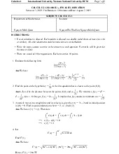
Đề thi cuối kỳ môn Calculus 1 | Trường Đại học Quốc tế, Đại học Quốc gia Thành phố Hồ Chí Minh
59 30 -
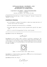
Đề thi cuối kỳ 2023 - 2024 môn Calculus 1 | Trường Đại học Quốc tế, Đại học Quốc gia Thành phố Hồ Chí Minh
53 27 -
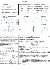
Note Calculus 1 Midterm - Calculus 1 | Trường Đại học Quốc tế, Đại học Quốc gia Thành phố HCM
693 347 -
Review final Calculus - Calculus 1 | Trường Đại học Quốc tế, Đại học Quốc gia Thành phố HCM
461 231 -
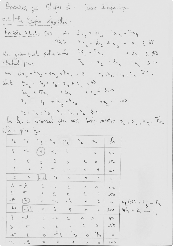
Chapter 2 - Calculus 1 | Trường Đại học Quốc tế, Đại học Quốc gia Thành phố HCM
316 158