Chapter 16 Vector Calculus - Calculus 1 | Trường Đại học Quốc tế, Đại học Quốc gia Thành phố HCM
Chapter 16 Vector Calculus - Calculus 1 | Trường Đại học Quốc tế, Đại học Quốc gia Thành phố HCM được sưu tầm và soạn thảo dưới dạng file PDF để gửi tới các bạn sinh viên cùng tham khảo, ôn tập đầy đủ kiến thức, chuẩn bị cho các buổi học thật tốt. Mời bạn đọc đón xem!
Môn: Calculus 1 (MA001IU) 44 tài liệu
Trường: Trường Đại học Quốc tế, Đại học Quốc gia Thành phố Hồ Chí Minh 1.9 K tài liệu
Tác giả:


Preview text:
Vector Calculus 16
Parametric surfaces, which are studied in
Section 16.6, are frequently used by
programmers creating animated films. In
this scene from Antz, Princess Bala is
about to try to rescue Z, who is trapped
in a dewdrop. A parametric surface
represents the dewdrop and a family of
such surfaces depicts its motion. One of
the programmers for this film was heard
to say, “I wish I had paid more attention
in calculus class when we were studying
parametric surfaces. It would sure have helped me today.” © Dreamworks / Photofest
In this chapter we study the calculus of vector fields. (These are functions that assign vectors to points in
space.) In particular we define line integrals (which can be used to find the work done by a force field in
moving an object along a curve). Then we define surface integrals (which can be used to find the rate
of fluid flow across a surface). The connections between these new types of integrals and the single,
double, and triple integrals that we have already met are given by the higher-dimensional versions of the
Fundamental Theorem of Calculus: Green’s Theorem, Stokes’ Theorem, and the Divergence Theorem. 1079 1080 CHAPTER 16 16.1 Vector Fields
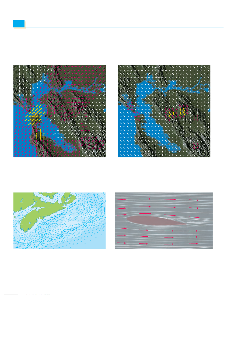
The vectors in Figure 1 are air velocity vectors that indicate the wind speed and direction
at points 10 m above the surface elevation in the San Francisco Bay area. We see at a
glance from the largest arrows in part (a) that the greatest wind speeds at that time occurred
as the winds entered the bay across the Golden Gate Bridge. Part (b) shows the very dif-
ferent wind pattern 12 hours earlier. Associated with every point in the air we can imagine
a wind velocity vector. This is an example of a velocity vector field. (a) 6:00 PM, March 1, 2010 (b) 6:00 AM, March 1, 2010
FIGURE 1 Velocity vector fields showing San Francisco Bay wind patterns
Other examples of velocity vector fields are illustrated in Figure 2: ocean currents and flow past an airfoil. Nova Scotia erle, 1974 photograph, W A ER N O dapted from A
(a) Ocean currents off the coast of Nova Scotia
(b) Airflow past an inclined airfoil
FIGURE 2 Velocity vector fields
Another type of vector field, called a force field, associates a force vector with each
point in a region. An example is the gravitational force field that we will look at in Example 4. V E C T O R F I E L D S 1081
In general, a vector field is a function whose domain is a set of points in (or ) and ⺢3 ⺢2
whose range is a set of vectors in V2 (or V3). 1 Definition Let be a set in
(a plane region). A vector field on is a ⺢2 D ⺢2
function F that assigns to each point 共x y
, 兲 in D a two-dimensional vector F共x y , 兲. y
The best way to picture a vector field is to draw the arrow representing the vector F(x,y)
F共x, y兲 starting at the point 共x y
, 兲 . Of course, it’s impossible to do this for all points 共x y , 兲,
but we can gain a reasonable impression of F by doing it for a few representative points in (x,y)
D as in Figure 3. Since F共x y
, 兲 is a two-dimensional vector, we can write it in terms of its
component functions P and Q as follows: 0 x F共x y
, 兲 苷 P共x, y兲 i ⫹ Q共x y
, 兲 j 苷 具P共x, y兲, Q共x y , 兲 典 or, for short,
F 苷 P i ⫹ Q j FIGURE 3
Notice that P and Q are scalar functions of two variables and are sometimes called scalar Vector field on R@
fields to distinguish them from vector fields. 2 Definition Let be a subset of . A vector field on is a function ⺢3 ⺢3 E F that
assigns to each point 共x y
, , z兲 in E a three-dimensional vector F共x y , , z兲. A vector field on
is pictured in Figure 4. We can express it in terms of its compo- z ⺢3 F F (x,y,z)
nent functions P, Q, and R as F共x y , , z兲 共 苷 P x y
, , z兲 i ⫹ Q共x, y, z兲 j ⫹ R共x, y, z兲 k 0 (x,y,z)
As with the vector functions in Section 13.1, we can define continuity of vector fields y
and show that F is continuous if and only if its component functions P, Q, and R are continuous. x
We sometimes identify a point 共x, y, z兲 with its position vector x and write 苷 具 x y , , z 典 FIGURE 4
F共x兲 instead of F共x y
, , z兲. Then F becomes a function that assigns a vector F共x兲 to a vec- Vector field on R# tor x. A vector field on is defined by ⺢2 EXAMPLE 1 v F共x y
, 兲 苷 ⫺y i ⫹ x j. Describe F by y
sketching some of the vectors F共x y , 兲 as in Figure 3. F(0,3) F(2,2)
SOLUTION Since F共1, 0兲 , we draw the vector 苷 j j starting at the point 共 苷 具 0, 1 典 1, 0兲 in
Figure 5. Since F共0, 1兲 , we draw the vector 具 苷 ⫺i
⫺1, 0 典 with starting point 共0, 1 . 兲 Con-
tinuing in this way, we calculate several other representative values of F共x y , 兲 in the table
and draw the corresponding vectors to represent the vector field in Figure 5. F(1,0) 0 x 共x y , 兲
F共x, y兲 共x y , 兲
F共x, y兲 共 兲 1, 0 具 0, 1 典 共⫺ 兲 1, 0 具 0, ⫺1典 共 兲 2, 2 具⫺2, 2 典 共⫺2, ⫺ 兲 2 具 2, ⫺2典 共 兲 3, 0 具 0, 3 典 共⫺ 兲 3, 0 具 0, ⫺3典 共 兲 0, 1 具 ⫺1, 0典 共0, ⫺ 兲 1 具 1, 0 典 共⫺ 兲 2, 2 具 ⫺2, ⫺2典 共2, ⫺ 兲 2 具 2, 2 典 FIGURE 5 共 兲 0, 3 具 ⫺3, 0典 共0, ⫺ 兲 3 具 3, 0 典
F(x,y)=_yi+xj 1082 CHAPTER 16
It appears from Figure 5 that each arrow is tangent to a circle with center the origin.
To confirm this, we take the dot product of the position vector x 苷 x i ⫹ y j with the
vector F共x兲 苷 F : 共x y , 兲
x ⴢ F共x兲 苷 共x i ⫹ y j兲 ⴢ 共⫺ 苷 y i ⫺ ⫹ xyj ⫹ 兲 yx 苷 0 This shows that F i 共 sx p , yerp
兲 endicular to the position vector 具x, yand 典 is therefore
tangent to a circle with center the origin and radius . Notice also that
ⱍxⱍ苷 sx2 ⫹ y2
ⱍF共x, y兲
ⱍ苷 s共⫺y兲2 ⫹ x2 苷 sx2 ⫹ y2 苷ⱍxⱍ
so the magnitude of the vector F共x, i y s e
兲 qual to the radius of the circle.
Some computer algebra systems are capable of plotting vector fields in two or three
dimensions. They give a better impression of the vector field than is possible by hand
because the computer can plot a large number of representative vectors. Figure 6 shows a
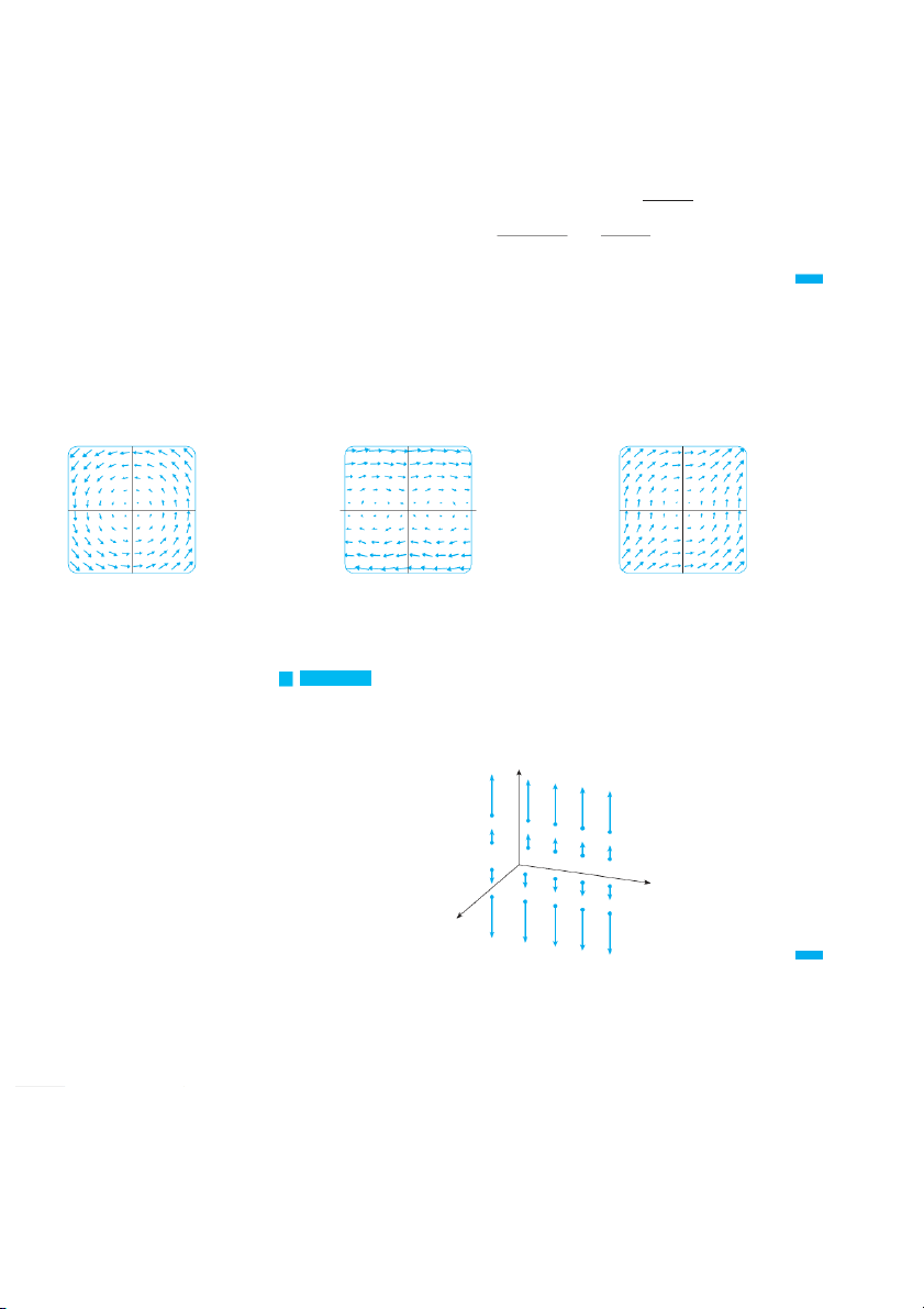
computer plot of the vector field in Example 1; Figures 7 and 8 show two other vector
fields. Notice that the computer scales the lengths of the vectors so they are not too long
and yet are proportional to their true lengths. 5 6 5 _5 5 _6 6 _5 5 _5 _6 _5 FIGURE 6 FIGURE 7 FIGURE 8 F(x, y)=k_y, xl F(x, y)=ky, sin xl
F(x, y)=k ln(1+¥), ln(1+≈ )l v Sketch the vector field on give ⺢3 EXAMPLE 2
n by F共x, y, z兲 . 苷 z k
SOLUTION The sketch is shown in Figure 9. Notice that all vectors are vertical and point
upward above the xy -plane or downward below it. The magnitude increases with the
distance from the xy-plane. z 0 y x FIGURE 9 F(x, y, z)=z k
We were able to draw the vector field in Example 2 by hand because of its particularly
simple formula. Most three-dimensional vector fields, however, are virtually impossible to VECTOR FIELDS 1083
sketch by hand and so we need to resort to a computer algebra system. Examples are
shown in Figures 10, 11, and 12. Notice that the vector fields in Figures 10 and 11 have simi-
lar formulas, but all the vectors in Figure 11 point in the general direction of the negative
y-axis because their y-components are all ⫺2. If the vector field in Figure 12 represents a
velocity field, then a particle would be swept upward and would spiral around the z-axis
in the clockwise direction as viewed from above. 1 1 5 z 0 z 0 z 3 _1 _1 1 _1 _1 _1 _1 0 _1 0 0 _1 0 0 0 x 1 y 1 1 x y 1 1 x y 1 FIGURE 10 FIGURE 11 FIGURE 12
F(x, y, z)=y i+z j+x k
F(x, y, z)=y i-2 j+x k y x z F(x, y, z)= i- j+ k z z 4
TEC In Visual 16.1 you can rotate the
EXAMPLE 3Imagine a fluid flowing steadily along a pipe and let V共x y , , b z e t 兲 he veloc-
vector fields in Figures 10–12 as well as
ity vector at a point 共x, y, . zTh
兲 en V assigns a vector to each point 共x y , , zin a 兲 certain additional fields.
domain E (the interior of the pipe) and so V is a vector field on ⺢ 3called a velocity field. z
A possible velocity field is illustrated in Figure 13. The speed at any given point is indi-
cated by the length of the arrow.
Velocity fields also occur in other areas of physics. For instance, the vector field in
Example 1 could be used as the velocity field describing the counterclockwise rotation of
a wheel. We have seen other examples of velocity fields in Figures 1 and 2. 0 y x
EXAMPLE 4Newton’s Law of Gravitation states that the magnitude of the gravitational
force between two objects with masses m and M is FIGURE 13 Velocity field in fluid flow ⱍFⱍ苷 mMG r 2
where r is the distance between the objects and G is the gravitational constant. (This
is an example of an inverse square law.) Let’s assume that the object with mass M is
located at the origin in ⺢ .
3 (For instance, M could be the mass of the earth and the origin
would be at its center.) Let the position vector of the object with mass be x
m 苷 具 x, y . , z 典 Then , so r 2 苷
. The gravitational force exerted on this second object acts ⱍxⱍ2 r 苷 ⱍxⱍ
toward the origin, and the unit vector in this direction is x ⫺ ⱍxⱍ
Therefore the gravitational force acting on the object at x 苷 具 x y , , i z s典 mMG 3 F共x兲 苷 ⫺ ⱍ x x ⱍ3
[Physicists often use the notation r instead of x for the position vector, so you may see 1084 CHAPTER 16
Formula 3 written in the form F 苷 ⫺共mMG兾r.]3 Th
兲re function given by Equation 3 is z
an example of a vector field, called the gravitational field, because it associates a vector
[the force F共 ]x w
兲ith every point x in space.
Formula 3 is a compact way of writing the gravitational field, but we can also write
it in terms of its component functions by using the facts that x 苷 x i ⫹ y j ⫹ z k and y 2 z2 :
ⱍxⱍ苷 sx2 ⫹ ⫹ x y ⫺mMGy ⫺mMGz F共x y , , z兲 苷 ⫺mMGx 共 i ⫹ j ⫹ k
x 2 ⫹ y 2 ⫹ z2 兲3兾2 共x 2 ⫹ y 2 ⫹ z2 兲3兾2 共x 2 ⫹ y 2 ⫹ z2 兲3兾2
The gravitational field F is pictured in Figure 14.
EXAMPLE 5 Suppose an electric charge Q is located at the origin. According to FIGURE 14
Coulomb’s Law, the electric force F共 e x xe
兲 rted by this charge on a charge q located at a Gravitational force field point 共x wy , it , h z po
兲 sition vector x 苷 具x y , , i z s典 4
F共x兲 苷qQ ⱍ x x ⱍ3
where is a constant (that depends on the units used). For like charges, we have qQ ⬎ 0
and the force is repulsive; for unlike charges, we have qQ ⬍ 0 and the force is attractive.
Notice the similarity between Formulas 3 and 4. Both vector fields are examples of force fields.
Instead of considering the electric force F, physicists often consider the force per unit charge: 1
E共x兲 苷F共x兲 苷Q x q ⱍxⱍ3 Then is a vector field on ⺢3 E
called the electric field of Q . Gradient Fields
If f is a scalar function of two variables, recall from Section 14.6 that its gradient ∇ f (or grad f ) is defined by ⵜf 共x y , 兲 苷 f 共 兲 共 x x, y i ⫹ fy x y , 兲 j Therefore
is really a vector field on ⺢2 ∇ f
and is called a gradient vector field. Likewise,
if f is a scalar function of three variables, its gradient is a vector field on ⺢3given by 4 ⵜf 共x y , , z兲 苷 f 共 共 x
x, y, z兲 i ⫹ fy
x, y, z兲 j ⫹ fz共x y , , z兲 k v
Find the gradient vector field of f 共x y
, 兲 苷 x 2 y . ⫺ P y l3 EXAMPLE 6 ot the gradient
vector field together with a contour map of f. How are they related? _4 4
SOLUTION The gradient vector field is given by ⭸ ⭸ ⵜ f f f 共x y , 兲 苷 ⭸ i ⫹
j 苷 2 x y i ⫹ 共x 2 ⫺ 3y 2 兲 j x ⭸y _4
Figure 15 shows a contour map of f with the gradient vector field. Notice that the gradi- FIGURE 15
ent vectors are perpendicular to the level curves, as we would expect from Section 14.6. VECTOR FIELDS 1085
Notice also that the gradient vectors are long where the level curves are close to each
other and short where the curves are farther apart. That’s because the length of the gradi-
ent vector is the value of the directional derivative of f and closely spaced level curves indicate a steep graph.
A vector field F is called a conservative vector field if it is the gradient of some scalar
function, that is, if there exists a function f such that F 苷 ∇ f . In this situation f is called
a potential function for . F
Not all vector fields are conservative, but such fields do arise frequently in physics. For
example, the gravitational field F in Example 4 is conservative because if we define f x y , , z 苷 mMG sx2 y 2 z2 then f f f x y , , z 苷 f i j k x y z 苷 mMGx mMGy mMGz i j k x 2 y 2 z2 3 2 x 2 y 2 z2 3 2 x 2 y 2 z2 3 2
苷 F x, y, z
In Sections 16.3 and 16.5 we will learn how to tell whether or not a given vector field is conservative. 16.1 Exercises
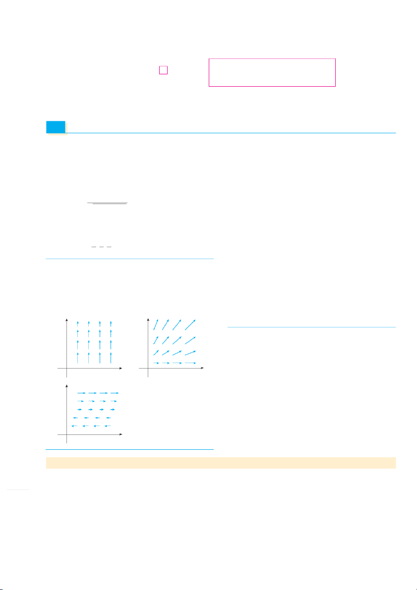
1–10 Sketch the vector field F by drawing a diagram like 13. F x y , 苷 y, y 2 Fig ure 5 or Figure 9. 14. F x y , 苷 cos x y , x 1. F x y , 苷 0.3 i 0.4 j 2. F x y , x苷 1 i y j 2 I 3 II 3 3. F x y , 苷 1 i y x j 4. F x y , 苷 y i x y j 2 5. F x y , 苷y i x j sx 2 y 2 _3 3 _3 3 i j 6. F x y , 苷y x sx 2 y 2 7. F x y , , z 苷 k _3 _3 8. F x y , , z 苷 y k III 3 IV 3 9. F x y , , z 苷 x k 10. F x y , , z 苷 j i _3 3 _3 3
11–14 Match the vector fields F with the plots labeled I – IV. Give reasons for your choices. 11. F x y , 苷 x, y _3 _3 12. F x y , 苷 y, x y
CAS Computer algebra system required
1. Homework Hints available at stewartcalculus.com 1086 CHAPTER 16
15–18 Match the vector fields F on ⺢3 with the plots labeled
29 –32 Match the functions f with the plots of their gradient
I–IV. Give reasons for your choices.
vector fields labeled I – IV. Give reasons for your choices. 15. F共x y
, , z兲 苷 i ⫹ 2 j ⫹ 3 k 16. F共x y
, , z兲 苷 i ⫹ 2 j ⫹ z k29. f 共x y
, 兲 苷 x 2 ⫹ y 2 30. f 共x y
, 兲 苷 x共x ⫹ y兲 17. F共x y
, , z兲 苷 x i ⫹ y j ⫹ 3 k 31. f 共x y
, 兲 苷 共x ⫹ y兲2 32. f 共x y
, 兲 苷 sin sx 2 ⫹ y 2 18. F共x y
, , z兲 苷 x i ⫹ y j ⫹ z k I 4 II 4 I II 1 1 _4 4 _4 4 0 z z 0 _1 _1 _4 _4 _1 0 0 _1 _1 0 1 x0 _1 y 1 1 x y 1 III 4 IV 4 III IV 1 1 _4 4 _4 4 z 0 z 0 _1 _1 _4 _4 _1 0 0 _1 _1 0 1 0 _1 y 1 1 x y 1 x
33. A particle moves in a velocity field V共x, y兲 苷 具x2, x . ⫹ y 2 典
If it is at position 共2, 1at 兲time t , e 苷 st 3 imate its location at
CAS 19. If you have a CAS that plots vector fields (the command time t 苷 . 3.01
is fieldplotin Maple and PlotVectorFieldor
VectorPlotin Mathematica), use it to plot 34. At time t 苷 ,
1 a particle is located at position 共 . 1, 3If i 兲 t moves in a velocity field F共x y
, 兲 苷 共 y 2 ⫺ 2 x y兲 i ⫹ 共3x y ⫺ 6 x 2 兲 j
Explain the appearance by finding the set of points 共x y , 兲
F共x, y兲 苷 具 xy ⫺ 2, y 2 ⫺ 10 典
such that F共x y , 兲 . 苷 0
find its approximate location at time t 苷 . 1.05
CAS 20. Let F共x兲 苷 共r 2 , ⫺ w 2rher 兲 e x x 苷 and
具 x, y典 . Usre a 苷 ⱍxⱍ
35. The flow lines (or streamlines) of a vector field are the
CAS to plot this vector field in various domains until you can
paths followed by a particle whose velocity field is the
see what is happening. Describe the appearance of the plot
given vector field. Thus the vectors in a vector field are tan-
and explain it by finding the points where F x 共 兲 . 苷 0 gent to the flow lines. 21–24
(a) Use a sketch of the vector field F共x y
, 兲 苷 x i ⫺ to y j
Find the gradient vector field of f .
draw some flow lines. From your sketches, can you 21. f 共x y , 兲 苷 xe xy 22. f 共x y
, 兲 苷 tan共3x ⫺ 4y兲
guess the equations of the flow lines? 23. f 共x y
, , z兲 苷 sx 2 ⫹ y 2 ⫹ z 2
(b) If parametric equations of a flow line are x 苷 x共t兲, y 苷 y , 共 etxp
兲 lain why these functions satisfy the differ- 24. f 共x y
, , z兲 苷 x ln共 y ⫺ 2z兲
ential equa tions dx兾dt 苷 a
x nd dy兾dt 苷 . T ⫺ h y en solve
the differential equations to find an equation of the flow
line that passes through the point (1, 1).
25–26 Find the gradient vector field ∇ f of f and sketch it.
36. (a) Sketch the vector field F共x y
, 兲 苷 i ⫹ axnd j then sketch 25. f 共x y
, 兲 苷 x 2 ⫺ y 26. f 共x y
, 兲 苷 sx 2 ⫹ y2
some flow lines. What shape do these flow lines appear to have?
(b) If parametric equations of the flow lines are x 苷 x共t兲, 27 CAS
–28 Plot the gradient vector field of f together with a contour y 苷 y , 共 w t h
兲 at differential equations do these functions map of .
f Explain how they are related to each other.
satisfy? Deduce that dy兾dx 苷.x 27.
f 共x, y兲 苷 ln共1 ⫹ x 2 ⫹ 228. y 2 f 兲共x y
, 兲 苷 cos x ⫺ 2 sin y
(c) If a particle starts at the origin in the velocity field given
by F, find an equation of the path it follows. LINE INTEGRALS 1087 16.2 Line Integrals
In this section we define an integral that is similar to a single integral except that instead
of integrating over an interval a, ,
b we integrate over a curve . S
C uch integrals are called
line integrals, although “curve integrals” would be better terminology. They were invented
in the early 19th century to solve problems involving fluid flow, forces, electricity, and magnetism.
We start with a plane curve C given by the parametric equations 1 x 苷 x t y 苷 y t a t b P*i(x* i , y*
or, equivalently, by the vector equation r t y i ) 苷 x t i , y antd w j e assume that is a C Pi-1
smooth curve. [This means that P
r is continuous and r t . S 苷ee 0 Section 13.3.] If we i C
divide the parameter interval a, b into n subintervals ti 1 o , t f
i equal width and we let x 苷 苷 i x ti and yi y, th
tien the corresponding points Pi d x iiv , id yi e into Csubarcs n P P™ n with lengths s * 1,
s2, . . . , sn.(See Figure 1.) We choose any point Pi* x * i, yi in the ith P¡
subarc. (This corresponds to a point ti* in ti 1, t .i) Now if is
f any function of two vari-
ables whose domain includes the curve C , we evaluate f at the point x* * i, yi , multiply by P¸
the length si of the subarc, and form the sum 0 x t* n i t f x* * i, yi si a b i t t 苷1 i-1 i FIGURE 1
which is similar to a Riemann sum. Then we take the limit of these sums and make the fol-
lowing definition by analogy with a single integral.
2 Definition If f is defined on a smooth curve C given by Equations 1, then the
line integral of f along C is n
y f x, y ds 苷 lim f x* * i, yi si C n l i苷1 if this limit exists.
In Section 10.2 we found that the length of C is 2 2 L 苷 yb dx d ydt dt dt a
A similar type of argument can be used to show that if f is a continuous function, then the
limit in Definition 2 always exists and the following formula can be used to evaluate the line integral: 2 dy 2 3
y f x, y ds 苷f (x t y , ) dx t dt a yb C dt dt
The value of the line integral does not depend on the parametrization of the curve, pro-
vided that the curve is traversed exactly once as t increases from a to b. 1088 CHAPTER 16 The arc length function s is discussed in If s共 its t
兲he length of C between r an
共da 兲 , thern共t兲 Section 13.3.
ds 苷 冑冊2冉dy 冊2 ⫹ dt 冉 dx dt dt
So the way to remember Formula 3 is to express everything in terms of the parameter t:
Use the parametric equations to express x and y in terms of t and write ds as 冊2冉dy 冊2 ds 苷 冑冉dx ⫹ dt dt dt z In the special case where is the
C line segment that joins 共 to a 共 , 0 b 兲 , , 0 us 兲ing x as the
parameter, we can write the parametric equations of C as follows: x 苷 , x y 苷 , 0 a 艋 x 艋 .
b Formula 3 then becomes 0
y f共x, y兲 ds 苷f yb 共x, 0兲 dx C y C a f(x, y) (x, y)
and so the line integral reduces to an ordinary single integral in this case.
Just as for an ordinary single integral, we can interpret the line integral of a positive x
function as an area. In fact, if
f 共x, y , x 兲 f 艌共 0 x y , r 兲 ep
ds resents the area of one side of C
the “fence” or “curtain” in Figure 2, whose base is C and whose height above the point FIGURE 2 共isx fy , 共 兲 x .y , 兲
EXAMPLE 1 Evaluate x 共2 ⫹ x2y , 兲wh
ds ere C is the upper half of the unit circle C
x 2 ⫹ y 2 苷 . 1 y
SOLUTION In order to use Formula 3, we first need parametric equations to represent C.
Recall that the unit circle can be parametrized by means of the equations ≈+¥=1 (y˘0) x 苷 cos t y 苷 sin t
and the upper half of the circle is described by the parameter interval 0 艋 t 艋 .
(See Figure 3.) Therefore Formula 3 gives 0 x _1 1 FIGURE 3 y 共 冊2冉dy 冊2
2 ⫹ x 2y兲 ds 苷 y
共2 ⫹ cos2t sin t兲冑 ⫹ dt dt 冉dx C 0 dt
苷 y 共2 ⫹ cos2t sin t兲ssin2t ⫹ cos2t dt 0 苷 y y C¢ 冋 册 共 cos3t
2 ⫹ cos2t sin t兲 dt 苷 2t ⫺ 0 3 0 C∞ 苷 2 ⫹ 23 C£ C™
Suppose now that C is a piecewise-smooth curve; that is, C is a union of a finite num- C¡
ber of smooth curves C1, C2, . . . , Cn, where, as illustrated in Figure 4, the initial point of x
Ci⫹1 is the terminal point of Ci . Then we define the integral of f along C as the sum of the 0
integrals of f along each of the smooth pieces of C : FIGURE 4 A piecewise-smooth curve
y f共x, y兲 ds 苷f y共x y , 兲 ds ⫹ y f 共x y
, 兲 ds ⫹ ⭈ ⭈ ⭈ ⫹ y f 共x y , 兲 ds C C C C 1 2 n LINE INTEGRALS 1089
EXAMPLE 2Evaluate x 2x d ,
s where Cconsists of the arc C1 of the parabola y 苷 x 2 C from 0, 0 to fo
1, 1 llowed by the vertical line segment fro Cm to 2 1, 1 . 1, 2 y
SOLUTION The curve C is shown in Figure 5. C1 is the graph of a function of x , so we can
choose x as the parameter and the equations for C1 become (1, 2) C™ y 苷 x 2 x 苷 x 0 x 1 (1, 1) Therefore C¡ (0, 0) x y dx2 dy 2 2x ds 苷 y12x dx 苷 y12xs1 4x 2 dx C1 0 0 dx dx FIGURE 5 苷 1 ⴢ 2 1 苷 5s5 1 4 1 4x 2 3 2 ] 3 0 6 C=C¡ 傼 C™
On C2 we choose y as the parameter, so the equations of C2 are x 苷 1 y 苷 y 1 y 2 2 2 and y dx dy 2x ds 苷 y22 1
dy 苷 y22 dy 苷 2 C 1 2 1 dy dy Thus
y 2x ds 苷 y2x ds y 2x ds 苷5s5 1 2 C C1 C2 6
Any physical interpretation of a line integral x f x, y de
ds pends on the physical inter- C pretation of the function . S f uppose that x y
, represents the linear density at a point x y
, of a thin wire shaped like a curve C. Then the mass of the part of the wire from Pi 1
to Pi in Figure 1 is approximately x*, y* i a
si nd so the total mass of the wire is approx- i imately x*, y* i .
siBy taking more and more points on the curve, we obtain the mass i
m of the wire as the limiting value of these approximations: n m 苷 lim x *, y 苷 y i i* si x y , ds n l i苷1 C [For example, if f x y , 苷 2 x r 2 e
ypresents the density of a semicircular wire, then the
integral in Example 1 would represent the mass of the wire.] The center of mass of the
wire with density function is located at the point x, y, where 1 4 x 苷 y x x y , ds y 苷 1 y y x y , ds m C m C
Other physical interpretations of line integrals will be discussed later in this chapter.
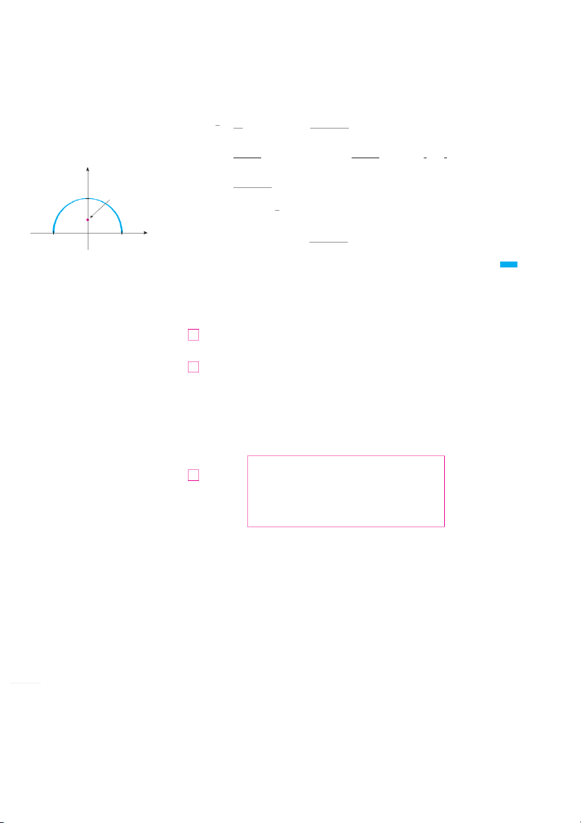
v EXAMPLE 3A wire takes the shape of the semicircle x2 y 2 苷 , 1 y 0 , and is
thicker near its base than near the top. Find the center of mass of the wire if the linear
density at any point is proportional to its distance from the line y 苷 . 1
SOLUTION As in Example 1 we use the parametrization x 苷 cos t, y 苷 sin t , 0 t ,
and find that ds 苷 dt. The linear density is x y , 苷 k 1 y 1090 CHAPTER 16
where k is a constant, and so the mass of the wire is m 苷 k 1 y ds 苷k y1 sin t 苷 dt k y [t cos t] 苷 0 k 2 C 0 From Equations 4 we have y 苷 1 y y x y , ds 苷 1 y y k 1 y ds m C k 2 C
苷 1 y sin t sin2t dt 苷 1 [ cos t 1 sin 2t] 2 t 1 4 0 2 0 2 y center of 苷 4 1 2 2 mass
By symmetry we see that x 苷 , 0 so the center of mass is 0 x 4 _1 1 0, 0, 0.38 2 2 FIGURE 6 See Figure 6.
Two other line integrals are obtained by replacing s by either i x 苷 x or i i xi 1 y 苷 y
in Definition 2. They are called the line integrals of i i yi 1
f along C with respect to x and y: n 5 y f x y , dx 苷 lim f x* * i, yi xi C n l i苷1 n 6 y f x y , d y 苷 lim f x* * i, yi yi C n l i苷1
When we want to distinguish the original line integral x f x, y fro ds m those in Equa - C
tions 5 and 6, we call it the line integral with respect to arc length.
The following formulas say that line integrals with respect to x and y can also be
evaluated by expressing everything in terms of : x t ,
苷 x yt 苷, ydxt 苷 x t , dt dy 苷 y t . dt 7 y f x y ,
dx 苷 f (x t y , ) t x t dt a yb C y f x y ,
dy 苷 f (x t y , ) t y t dt a yb C
It frequently happens that line integrals with respect to x and y occur together. When
this happens, it’s customary to abbreviate by writing y P x y , dx y Q x y ,
dy 苷 y P x, y dx Q x, y dy C C C
When we are setting up a line integral, sometimes the most difficult thing is to think of
a parametric representation for a curve whose geometric description is given. In particular,
we often need to parametrize a line segment, so it’s useful to remember that a vector rep- LINE INTEGRALS 1091
resentation of the line segment that starts at r0 and ends at r1 is given by 8 r t 苷 1 t r0 t r1 0 t 1 (See Equation 12.5.4.) y
v EXAMPLE 4Evaluate x y2 dx x d ,y where (a) C 苷 C1is the line segment from C 5, to 3 0, 2 and (b)
is the arc of the parabola x 苷 4 f y r2 C 苷 C2 om 5, 3 (0, 2) to . 0, 2 (See Figure 7.) C™ C¡ SOLUTION 0 x
(a) A parametric representation for the line segment is 4 x=4-¥ x 苷 5t 5 y 苷 5t 3 0 t 1 (_5, _3) (Use Equation 8 with r 苷 0 5, and 3 r 苷 1 .) 0, 2 Then dx 苷 5 , dt dy 苷 5 , dt and Formulas 7 give FIGURE 7
y y2 dx x dy 苷 y1 5t 3 2 5 dt 5t 5 5 dt C 0 1
苷 5 y1 25t2 25t 4 dt 0 1 25t 2 苷 25t 3 5 4t 苷 5 3 2 6 0
(b) Since the parabola is given as a function of y, let’s take y as the parameter and write C2 as x 苷 4 y 2 y 苷 y 3 y 2 Then dx 苷
2y dy and by Formulas 7 we have
y y2 dx x dy 苷 y2y2 2y dy 4 y 2 dy C 3 2 苷 y2 2y 3 y 2 4 dy 3 2 y 3 苷 y 4 4y 苷 40 5 2 3 6 3
Notice that we got different answers in parts (a) and (b) of Example 4 even though the
two curves had the same endpoints. Thus, in general, the value of a line integral depends
not just on the endpoints of the curve but also on the path. (But see Section 16.3 for con-
ditions under which the integral is independent of the path.)
Notice also that the answers in Example 4 depend on the direction, or orientation, of the curve. If de Cn 1 otes the line segment from to 0, 2
5, 3, you can verify, using the parametrization x 苷 t 5 y 苷 2 5t 0 t 1 that
y y2 dx x dy 苷 56 C1 1092 CHAPTER 16 B
In general, a given parametrization x 苷 , x y 苷 t y ,t a t
b , determines an orien-
tation of a curve C, with the positive direction corresponding to increasing values of the C
parameter t. (See Figure 8, where the initial point A corresponds to the parameter value a A
and the terminal point Bcorresponds to t 苷 . b)
If C denotes the curve consisting of the same points as C but with the opposite ori-
entation ( from initial point B to terminal point A in Figure 8), then we have t a b B f x, y dx 苷 y f x y , dx y f x y , dy 苷 y f x y , dy y C C C C _C
But if we integrate with respect to arc length, the value of the line integral does not change A
when we reverse the orientation of the curve: FIGURE 8
y f x, y ds 苷 y f x, y ds C C
This is because si is always positive, whereas xi and yi change sign when we reverse the orientation of C. Line Integrals in Space
We now suppose that C is a smooth space curve given by the parametric equations
x 苷 x t y 苷 y t z 苷 z t a t b
or by a vector equation r t 苷 x t i y t j . If z ft is a
k function of three variables
that is continuous on some region containing C, then we define the line integral of f
along C (with respect to arc length) in a manner similar to that for plane curves: n
y f x, y, z ds 苷 lim f x* * *
i, yi , zi si C n l i苷1
We evaluate it using a formula similar to Formula 3: 9 y dx2 dy 2 dz 2 f x, y, z
ds 苷f (x t y , t , )z t dt a yb C dt dt dt
Observe that the integrals in both Formulas 3 and 9 can be written in the more compact vector notation
ybf r t r tdt a For the special case f x y , , z , 苷 w 1 e get
y ds 苷 ybr tdt 苷 L C a
where L is the length of the curve C (see Formula 13.3.3). LINE INTEGRALS 1093
Line integrals along C with respect to x, y, and z can also be defined. For example, n y f x y , , z dz 苷 lim f x* * * z
i, yi , zi i C n l i苷1 苷 ybf(x t y , t , )z t t dt a
Therefore, as with line integrals in the plane, we evaluate integrals of the form 10 y P x y , , z dx Q x, y, z dy R x, y, z dz C
by expressing everything , x, y ,
z d, x d, ydz in terms of the parameter t.
v EXAMPLE 5Evaluate x y sin z ,
ds where C is the circular helix given by the equa- C
tions x 苷 cos , ty 苷 sin ,t z 苷 , t 0 t 2 . (See Figure 9.) SOLUTION Formula 9 gives 6 y d 2 x dy 2 dz 2
y sin z ds 苷 y2 sin t sin t dt 4 C 0 dt dt dt z 苷 2
y2sin2tssin2t cos2t 1 dt 苷 s2 y2 12 1 cos 2t dt 0 0 C 0 苷 s2 2 [t 1 sin 2t] 苷 s2 2 2 0 _1 _1 0 0 EXAMPLE 6Evaluate y x
x y dx z dy x d ,z where C consists of the line segment C1 C 1 1 from to
2, 0, 0 3, 4, 5, followed by the vertical line segment f Cr2om 3, 4, 5 to . 3, 4, 0 FIGURE 9
SOLUTION The curve C is shown in Figure 10. Using Equation 8, we write C1 as z r t 苷 1 t 2, 0, 0 t 3, 4, 5 苷 2 t, 4t, 5t (3, 4, 5) or, in parametric form, as C¡ C™ x 苷 2 t y 苷 4t z 苷 5t 0 t 1 0 (2, 0, 0) y Thus (3, 4, 0) x
y y dx z dy x dz 苷 y1 4t dt 5t 4 dt 2 t 5 dt C1 0 FIGURE 10 1 苷 y1 t 2 10 29t dt 苷 10t 29 苷 24.5 0 2 0
Likewise, C2 can be written in the form r t 苷 1 t 3, 4, 5 t 3, 4, 0 苷 3, 4, 5 5t or x 苷 3 y 苷 4 z 苷 5 5t 0 t 1 1094 CHAPTER 16
Then dx 苷 0 苷 d , y so
y y dx z dy x dz 苷 y13 5 dt 苷 15 C 0 2
Adding the values of these integrals, we obtain
y y dx z dy x dz 苷 24.5 15 苷 9.5 C
Line Integrals of Vector Fields
Recall from Section 5.4 that the work done by a variable force f x in moving a particle
from a to b along the -
x axis is W 苷 xbf x . d T
x hen in Section 12.3 we found that the a
work done by a constant force F in moving an object from a point P to another point Q in l
space is W 苷 F ⴢ ,
Dwhere D 苷 PQis the displacement vector. Now suppose that
is a continuous force field on ⺢ ,3 F 苷 P i Q j R k such as the
gravitational field of Example 4 in Section 16.1 or the electric force field of Example 5 in
Section 16.1. (A force field on ⺢ c
2 ould be regarded as a special case where R 苷 0 and P
and Q depend only on x and y.) We wish to compute the work done by this force in mov-
ing a particle along a smooth curve C. z
We divide C into subarcs Pi P 1 i with lengths
si by dividing the parameter interval a b
, into subintervals of equal width. (See Figure 1 for the two-dimensional case or F(x* i , y* i , z* i )
Figure 11 for the three-dimensional case.) Choose a point P * * i* x *
i, yi , zi on the ith subarc T(t* i )
corresponding to the parameter value t* i . If
si is small, then as the particle moves from Pi-1
Pi 1 to Pailong the curve, it proceeds approximately in the direction of T t*i , the unit tan- Pi gent vector at P*
i . Thus the work done by the force F in moving the particle from Pi 1 to 0 Pn Pi is approximately P*i(x* i , y* i , z* i ) y F x * * * ⴢ * 苷 * * * ⴢ *
i, yi , zi si T ti F, y x i i, zi T ti si x P¸
and the total work done in moving the particle along C is approximately FIGURE 11 n 11 F x * * * ⴢ * * * i , yi , zi T xi , yi , zi si i苷1 where T x y , is ,
zthe unit tangent vector at the point x y
, , z on C. Intuitively, we see that
these approximations ought to become better as n becomes larger. Therefore we define the
work W done by the force field F as the limit of the Riemann sums in 11 , namely, 12
W 苷 y F x y , , z ⴢ T x y , , z
ds 苷 y F ⴢ T ds C C
Equation 12 says that work is the line integral with respect to arc length of the tangen tial component of the force. If the curve is given
C by the vector equation r t 苷 x t i y t j , t z hen t k T t
苷 r rt ,t so using Equation 9 we can rewrite Equation 12 in the form r t
W 苷 F r t ⴢ r tdt 苷 yb ybF r t ⴢ r t dt a r t a LINE INTEGRALS 1095
This integral is often abbreviated as x F ⴢ d a
r nd occurs in other areas of physics as well. C
Therefore we make the following definition for the line integral of any continuous vector field.
13 Definition Let F be a continuous vector field defined on a smooth curveC
given by a vector function r t, a t
b . Then the line integral of F along C is
y F ⴢ dr 苷 ybF r t ⴢ r t
dt 苷 y F ⴢ T ds C a C
When using Definition 13, bear in mind that F r t is just an abbreviation for F , s x o twe , e y val t uat , e z t sim F ply r bty putting x , 苷 x y 苷 t , yand t z 苷 z t in the expression for F x . N y , , o
z tice also that we can formally write dr 苷 r t . dt
Figure 12 shows the force field and the curve in EXAMPLE 7Find the work done by the force field F x y , 苷 x2 i x i
y nj moving a par-
Example 7. The work done is negative because ticle along the quarter-circle r t 苷 cos t i si , n 0 t t j . 2
the field impedes movement along the curve.
SOLUTION Since x 苷 cos t and y 苷 sin t , we have y 1 F r t 苷 cos2t i
cos t sin t j and r t 苷 sin t i cos t j Therefore the work done is y 2
F ⴢ dr 苷 y2F r t ⴢ r t
dt 苷 2 cos2t sin t dt 0 y C 0 0 1 x 2 苷 cos3t 2 苷 2 FIGURE 12 3 3 0
NOTE Even though x F ⴢ dr 苷 x F ⴢ T a n
dsd integrals with respect to arc length are C C
unchanged when orientation is reversed, it is still true that
Figure 13 shows the twisted cubic C in
Example 8 and some typical vectors acting at three points on . C
y F ⴢ dr 苷 y F ⴢ dr C C 2
because the unit tangent vector T is replaced by its negative when C is replaced by C. 1.5 F{r (1)}
EXAMPLE 8Evaluate x F ⴢ d,
r where F x y , , z 苷 xy i yz j a zn x d k is C the C z 1 twisted cubic given by (1, 1, 1) F C z {r(3/4)} 苷 t3 y 苷 t 2 x 苷 t 0 t 1 0.5 SOLUTION We have 0 F{r(1 /2)} 0 r t 苷 t i t 2 j t k 3 y 1 22 1 0 r t 苷 i 2t j 3t 2 k x FIGURE 13 F r t 苷 t3 i t j 5 t 4 k 1096 CHAPTER 16 Thus
y F ⴢ dr 苷 y1F r t ⴢ r t dt C 0 1 苷 y1 5t 7 t 3 5t 6 dt 苷 t 4 苷 27 0 4 7 28 0
Finally, we note the connection between line integrals of vector fields and line integrals
of scalar fields. Suppose the vector field F on ⺢ 3 is given in component form by the equa-
tion F 苷 P i Q j R .
k We use Definition 13 to compute its line integral along C :
y F ⴢ dr 苷 ybF r t ⴢ r t dt C a
苷 yb P i Q j R k ⴢ(x t i y t j z)dt t k a
苷 yb[P(x t y , t , )zx t t ( Q x t y , t , )zy t t ( R x t y , t , ) z t t]dt a
But this last integral is precisely the line integral in 10 . Therefore we have
y F ⴢ dr 苷 y P dx Q dy R dz
where F 苷 P i Q j R k C C
For example, the integral x y dx z dy
x dz in Example 6 could be expressed as C x F ⴢ d w r here C F x y , , z 苷 y i z j x k 16.2 Exercises
1–16 Evaluate the line integral, where C is the given curve. 9. x xyz , ds C 1. x y 3 ,
ds C: x 苷 t 3, y 苷 t, 0 t 2
C: x 苷 2 sin t, y 苷 t, z 苷 2 cos t, 0 t C 10. x xyz2 , ds 2. x xy ,
ds C: x 苷 t 2, y 苷 2t, 0 t 1 C C
C is the line segment from 1, 5, 0 to 1, 6, 4 3. x x y 4 ,
ds C is the right half of the circle x 2 2 y 苷 16 11. x xe yz , ds C C
C is the line segment from (0, 0, 0) to (1, 2, 3)
4. x x sin y d ,s C is the line segment from 0, 3to 4, 6 C 12. x x 2 y 2 z2 , ds C 5. x (x2y3 sx ) dy, :
C x 苷 ,t y 苷 c , os 2 t z 苷 sin , 2 t 0 t 2 C
C is the arc of the curve y 苷 sx from 1, 1 to 4, 2 13. x xye yz d , y :
C x 苷 ,t y 苷 ,
t 2 z 苷 ,t 3 0 t 1 C 6. x e x d , x 14. x y dx z dy x d , z C C
C is the arc of the curve x 苷 y 3from 1, 1to 1, 1 :
C x 苷 st , y 苷 t, z 苷 t ,2 1 t 4 7. x x 2y dx x 2 , d y co
C nsists of line segments from 15. x z2 dx x 2 d y y 2 d ,
z C is the line segment from 1, 0, 0 C C 0, 0to an 2, 1 d from to 2, 1 3, 0 to 4, 1, 2 16. x z z z 8. x y dx x d y x , y d consis C ts of line x 2 dx y 2 d ,
y C consists of the arc of the circle C C segments from 0, 0, 0 to an 1, 0, 1 d from to 1, 0, 1 x 2 y 2 苷 4 from 2, 0 to fo
0, 2 llowed by the line segment 0, 1, 2 from 0, 2 to 4, 3
; Graphing calculator or computer required Co
CAS mputer algebra system required
1. Homework Hints available at stewartcalculus.com LINE INTEGRALS 1097
17. Let Fbe the vector field shown in the figure.
24. x F ⴢ d, rwhere F x y , , z 苷 y sin z i z sin x j x sin y k C
(a) If C is the vertical line segment from to , 1 3, 3 3, 3 and r t 苷 cos t i sin t j sin 5 , t k 0 t
determine whether x F ⴢ d i
r s positive, negative, or zero. C1
(b) If C is the counterclockwise-oriented circle with radius 3 25. x x sin y z , w dshere ha
Cs parametric equations x , 苷 t2 2 C 3 4
and center the origin, determine whether x F ⴢ d i r s posi-
y 苷 t , z 苷 t, 0 t 5 C2 tive, negative, or zero. 26. x ze xy , ds where h
C as parametric equations x 苷 , t y 苷 ,t 2 C z 苷 t y e , 0 t 1 3 2
CAS27–28 Use a graph of the vector field F and the curve C to guess
whether the line integral of F over C is positive, negative, or zero. 1
Then evaluate the line integral. 0 x 27. F x y , 苷 x y i , x y j _3 _2 _1 1 2 3 C x2 2 _1 is the arc of the circle
y 苷 4 traversed counter clock- wise from (2, 0) to 0, 2 _2 y 28. F x y , 苷 x i j , _3 sx 2 y 2 sx 2 y 2
C is the parabola y 苷 1 x 2from 1, 2to (1, 2)
18. The figure shows a vector field F and two curves C1 and C .2
Are the line integrals of F over C x
1 and C2 positive, negative,
29. (a) Evaluate the line integral F ⴢ , d rwhere C or zero? Explain. F x y , 苷 ex 1 i x a y n j d is C given by r t 苷 t2 i t, 3 j 0 t .1 y ;
(b) Illustrate part (a) by using a graphing calculator or com-
puter to graph C and the vectors from the vector field C¡
corresponding to t 苷 , 0 1 s , 2 and 1 (as in Figure 13). C™
30. (a) Evaluate the line integral x F ⴢ , d rwhere C F x y , , z 苷 x i z j y an k d is C given by r t 苷 2t i 3t j t , 2 k 1 t .1 x ;
(b) Illustrate part (a) by using a computer to graph a Cnd
the vectors from the vector field corresponding to t 苷 1 and 1 (as in Figure 13). 2
CAS 31. Find the exact value of x x 3y 2z , w ds here is C the curve with C
parametric equations x 苷 e t cos 4 ,t y 苷 e t sin 4 , t z 苷 e ,t 0 t 2 .
19 –22 Evaluate the line integral x F ⴢ d, rwhere i C s given by the C 32. vector function
(a) Find the work done by the force field F x y , 苷 x2 i x y j r .t
on a particle that moves once around the circle 19. F x y , 苷 xy i 3 , y 2 j x 2
y 2 苷 4 oriented in the counter-clockwise direction. r t 苷 11t4 i t , 3 j 0 t 1 CAS
(b) Use a computer algebra system to graph the force field and 20. F x y , , z 苷 x y i y z , j z2 k
circle on the same screen. Use the graph to explain your r t 苷 t2 i t 3 j t 2, k 0 t 1 answer to part (a). 21. F x y , , z 苷 sin x i cos y j x ,z k
33. A thin wire is bent into the shape of a semicircle x 2 y 2 苷 , 4 r t 苷 t3 i t 2 j t, k 0 t 1 x
0. If the linear density is a constant k, find the mass and center of mass of the wire. 22. F x y , , z 苷 x i y j x ,y k r t 苷 cos t i sin t j , t k 0 t
34. A thin wire has the shape of the first-quadrant part of the
circle with center the origin and radius a. If the density function is x y , 苷 ,k f x i
ynd the mass and center of mass
23–26 Use a calculator or CAS to evaluate the line integral correct of the wire. to four decimal places.
35. (a) Write the formulas similar to Equations 4 for the center of 23. x F , ⴢ w d h
r ere F x, y 苷 xy i sin a ynjd mass
x, y, zof a thin wire in the shape of a space curve C C r t 苷 et i e , t 2 1 j t 2
if the wire has density function x y , , .z 1098 CHAPTER 16
(b) Find the center of mass of a wire in the shape of the helix
45. A 160-lb man carries a 25-lb can of paint up a helical staircase
x 苷 2 sin ,t y 苷 2 cos, t z 苷 ,
3t 0 艋 t 艋 , 2 if the density
that encircles a silo with a radius of 20 ft. If the silo is 90 ft is a constant . k
high and the man makes exactly three complete revolutions
climbing to the top, how much work is done by the man
36. Find the mass and center of mass of a wire in the shape of the against gravity?
helix x 苷 ,t y 苷 cos ,
t z 苷 sin, t 0 艋 t 艋 , 2 if the density at
any point is equal to the square of the distance from the origin.
46. Suppose there is a hole in the can of paint in Exercise 45 and
9 lb of paint leaks steadily out of the can during the man’s
37. If a wire with linear density 共x, l y ies 兲 along a plane curve C, ascent. How much work is done?
its moments of inertia about the x- and y-axes are defined as
47. (a) Show that a constant force field does zero work on a
particle that moves once uniformly around the circle I 苷 y 苷 y x y 2 共x y , 兲 ds Iy x 2 共x y , 兲 ds
x 2 ⫹ y 2 苷 . 1 C C
(b) Is this also true for a force field F共x兲 , 苷 w k h x ere is a k
Find the moments of inertia for the wire in Example 3.
constant and x 苷 具x, ? y 典
38. If a wire with linear density 共x, y, l z ies 兲 along a space curve
48. The base of a circular fence with radius 10 m is given by ,
C its moments of inertia about the x-, - y , and - z axes are
x 苷 10 cos t, y 苷 10 sin .t The height of the fence at position defined as 共x iy , s g 兲 iven by the function 共 h x y , 兲 苷 4 ⫹ 共 0.01 , x s2o⫺ y 2兲
the height varies from 3 m to 5 m. Suppose that 1 L of paint 2
I 苷 y 共 y2 ⫹ z2兲
共x, y, z兲 ds
covers 100 m . Sketch the fence and determine how much paint x C
you will need if you paint both sides of the fence.
49. If C is a smooth curve given by a vector function r共 , I 苷 y共 t兲 y x 2 ⫹ z2 兲
共x, y, z兲 ds C a 艋 t 艋 ,
b and vis a constant vector, show that I 共 z 苷 y x 2 ⫹ y 2 兲
共x, y, z兲 ds
y v ⴢ dr 苷 v ⴢ 关r共b兲 ⫺ r共a兲兴 C C 50.
Find the moments of inertia for the wire in Exercise 35.
If C is a smooth curve given by a vector function r共 ,t兲 a 艋 t 艋 , b show that
39. Find the work done by the force fieldF共x y
, 兲 苷 x i ⫹ 共 y ⫹ 2兲 j
in moving an object along an arch of the cycloid
y r ⴢ dr 苷 1[ⱍr共 兲
bⱍ2 ⫺ ⱍr共a兲 ⱍ2] 2
r共t兲 苷 共t ⫺ sin t兲 i ⫹ 共1 ,
⫺ cos t兲 j 0 .艋 t 艋 2 C
51. An object moves along the curve C shown in the figure from
40. Find the work done by the force field F共x y
, 兲 苷 x 2 i ⫹ ye oxnj
(1, 2) to (9, 8). The lengths of the vectors in the force field F
a particle that moves along the parabola x 苷 y 2 ⫹ 1 from 共1, 0兲
are measured in newtons by the scales on the axes. Estimate to 共 .兲 2, 1
the work done by F on the object.
41. Find the work done by the force field y F共x y
, , z兲 苷 具 x ⫺ y 2, y ⫺ z2, z o ⫺ n x 2a p 典 article that moves (meters)
along the line segment from 共 t 0, 0, 1 o 兲 共 . 2, 1, 0兲 C
42. The force exerted by an electric charge at the origin on a
charged particle at a point 共x y , , w z it 兲 h position vector r 苷 具 x y , , i z s 典 F共r兲 苷 w Krher 兾 e is a constant. (See ⱍr ⱍ3 K
Example 5 in Section 16.1.) Find the work done as the particle
moves along a straight line from 共 t 2, 0, 0 o 兲 共 . 2, 1, 5兲 C
43. The position of an object with mass m at time t is 1
r共t兲 苷 at 2 i ⫹ ,
bt 3 j 0 艋 t .艋 1 0 1 x
(a) What is the force acting on the object at time t? (meters)
(b) What is the work done by the force during the time interval 0 艋 t 艋 ? 1
52. Experiments show that a steady current I in a long wire pro -
44. An object with mass m moves with position function
duces a magnetic field B that is tangent to any circle that lies in
r共t兲 苷 a sin t i ⫹ b cos t j ⫹ ,
ct k 0 艋 t 艋 . 兾 F 2 ind the work
the plane perpendicular to the wire and whose center is the axis
done on the object during this time period.
of the wire (as in the figure). Ampère’s Law relates the electric
THE FUNDAMENTAL THEOREM FOR LINE INTEGRALS 1
current to its magnetic effects and states that I
y B ⴢ dr 苷 0I C
where I is the net current that passes through any surface
bounded by a closed curve C, and 0 is a constant called the
permeability of free space. By taking C to be a circle with radius ,
r show that the magnitude B 苷 B of the magnetic
field at a distance r from the center of the wire is B B 苷 0 I 2 r
16.3 The Fundamental Theorem for Line Integrals
Recall from Section 4.3 that Part 2 of the Fundamental Theorem of Calculus can be writ- ten as 1 ybF x dx 苷 F b F a a
where F is continuous on a . b
, We also called Equation 1 the Net Change Theorem: The
integral of a rate of change is the net change.
If we think of the gradient vector ∇ f of a function f of two or three variables as a sort
of derivative of f, then the following theorem can be regarded as a version of the Funda-
mental Theorem for line integrals.
2 Theorem Let C be a smooth curve given by the vector function r ,t a t .b
Let f be a differentiable function of two or three variables whose gradient vector y
∇ f is continuous on C. Then A(x¡, y¡) B(x™, y™
y f ⴢ dr 苷 f r b f r a C 0 C x
NOTE Theorem 2 says that we can evaluate the line integral of a conservative vector
field (the gradient vector field of the potential function f ) simply by knowing the value of
f at the endpoints of C . In fact, Theorem 2 says that the line integral of ∇ f is the net (a)
change in f. If f is a function of two variables and C is a plane curve with initial point z
A x1, y1 and terminal point B x2 , , a
y2s in Figure 1, then Theorem 2 becomes C
y f ⴢ dr 苷 f x2, y2 f x1, y1 A(x¡, y¡, z¡) C B(x™, y™
If f is a function of three variables and C is a space curve joining the point A x z 1, y , 1 1 0
to the point B x2, y2, z , 2 then we have y x
y f ⴢ dr 苷 f x z z 2, y2, 2 f x1, y , 1 1 C (b) FIGURE 1
Let’s prove Theorem 2 for this case. CURL AND DIVERGENCE 1115
30. Complete the proof of the special case of Green’s Theorem
Here R is the region in the xy-plane that corresponds to the by proving Equation 3.
region S in the u -
v plane under the transformation given by 苷 苷 31. x t u, , v y h .u, v
Use Green’s Theorem to prove the change of variables
formula for a double integral (Formula 15.10.9) for the case
[Hint: Note that the left side is A Rand apply the first
part of Equation 5. Convert the line integral over Rto a where f x y , : 苷 1
line integral over Sand apply Green’s Theorem in the yy x, y dx dy 苷 yy du dv u - v plane.] u, v R S 16.5 Curl and Divergence
In this section we define two operations that can be performed on vector fields and that
play a basic role in the applications of vector calculus to fluid flow and electricity and mag-
netism. Each operation resembles differentiation, but one produces a vector field whereas
the other produces a scalar field. Curl
If F 苷 P i Q j
R k is a vector field on ⺢ 3 and the partial derivatives of , P , Q and R
all exist, then the curl of F is the vector field on ⺢ 3 defined by Q R P P Q 1 curl F 苷 R y i j k z z x x y
As an aid to our memory, let’s rewrite Equation 1 using operator notation. We intro-
duce the vector differential operator ∇ (“del”) as ∇ 苷 i j k x y z
It has meaning when it operates on a scalar function to produce the gradient of f : f f f f f ∇f 苷 i j k 苷 f i j k x y z x y z
If we think of ∇ as a vector with components , x , an yd , we c zan also consider
the formal cross product of ∇ with the vector field F as follows: i j k F 苷 x y z P Q R Q R P 苷 R P Q y i j k z z x x y 苷 curl F
So the easiest way to remember Definition 1 is by means of the symbolic expression 2 curl F 苷 ∇ F 1116 CHAPTER 16
EXAMPLE 1 If F x y , , z 苷 xz i x yz j y, 2 fi knd cur .l F
SOLUTION Using Equation 2, we have i j k curl F 苷 F 苷 x y z xz xyz y 2 苷 y 2 y 2 y z xyz i x z xz j
CAS Most computer algebra systems have com-
mands that compute the curl and divergence of
vector fields. If you have access to a CAS, use
these commands to check the answers to the xyz x xz k
examples and exercises in this section. y 苷 2y xy i 0 x j yz 0 k 苷 y 2 x i x j yz k
Recall that the gradient of a function f of three variables is a vector field on ⺢ 3 and so
we can compute its curl. The following theorem says that the curl of a gradient vector field is 0 .
3 Theorem If f is a function of three variables that has continuous second-order partial derivatives, then curl f 苷 0 PROOF We have i j k
Notice the similarity to what we know from Section 12.4: a a 苷 0 for every curl f 苷 f 苷x y z three-dimensional vector . a f f f x y z 2 2 2 2 f 2 f 2f 苷 f f f y z i j k z y z x x z x y y x 苷 0 i 0 j 0 k 苷 0 by Clairaut’s Theorem.
Since a conservative vector field is one for which F 苷 ∇ f , Theorem 3 can be re phrased as follows:
Compare this with Exercise 29 in
If F is conservative, then curl F 苷 . 0 Section 16.3.
This gives us a way of verifying that a vector field is not conservative. CURL AND DIVERGENCE 1117
v EXAMPLE 2Show that the vector field F x y , , z 苷 xz i x yz j y i 2 s k not conservative.
SOLUTION In Example 1 we showed that curl F 苷 y 2 x i x j yz k
This shows that curl F 苷 0 and so, by Theorem 3, F is not conservative.
The converse of Theorem 3 is not true in general, but the following theorem says the
converse is true if F is defined everywhere. (More generally it is true if the domain is
simply-connected, that is, “has no hole.”) Theorem 4 is the three-dimensional version
of Theorem 16.3.6. Its proof requires Stokes’ Theorem and is sketched at the end of Section 16.8.
4 Theorem If F is a vector field defined on all of ⺢3 whose component func-
tions have continuous partial derivatives and curl F 苷 ,
0 then F is a conservative vector field. v EXAMPLE 3 (a) Show that F x y , , z 苷 y2z3 i 2 x yz3 j 3x y 2z2 k
is a conservative vector field.
(b) Find a function f such that F 苷 . f SOLUTION
(a) We compute the curl of F : i j k curl F 苷 F 苷 x y z y 2z 3 2 x yz 3 3x y 2z 2 苷 6xyz2 6xyz2 i 3y 2z2 3y 2z2 j 2yz3 2yz3 k 苷 0
Since curl F 苷 0 and the domain of F is ⺢, 3 i
F s a conservative vector field by Theorem 4.
(b) The technique for finding f was given in Section 16.3. We have 5 fx x, y, z 苷 y2z3 6 fy x, y, z 苷 2xyz3 7 fz x y , , z 苷 3xy2z2
Integrating 5 with respect to x, we obtain 8 f x y , , z 苷 xy2z3 t y, z 1118 CHAPTER 16
Differentiating 8 with respect to y , we get f 共 z兲 y
x, y, z兲 苷 2 xyz3 ⫹ t 共 y , s y o , comparison
with 6 gives t 共y, z兲 . 苷Th 0 us t共y, z兲 an 苷 d共z兲 y h
fz共x, y, z兲 苷 3x y 2z2 ⫹ h⬘共z兲
Then 7 gives h⬘共z兲. Th 苷 er 0 efore
f 共x, y, z兲 苷 x y 2z3 ⫹ K
The reason for the name curl is that the curl vector is associated with rotations. One
connection is explained in Exercise 37. Another occurs when F represents the velocity curl F(x, y,
field in fluid flow (see Example 3 in Section 16.1). Particles near (x, y, z ) in the fluid tend
to rotate about the axis that points in the direction of curl F共x, y, ,z an 兲 d the length of this
curl vector is a measure of how quickly the particles move around the axis (see Figure 1). (x, y, z)
If curl F 苷 0 at a point ,
P then the fluid is free from rotations at P and F is called irro ta-
tional at P. In other words, there is no whirlpool or eddy at P. If curl F 苷 , 0 then a
tiny paddle wheel moves with the fluid but doesn’t rotate about its axis. If curl F 苷 , 0 the FIGURE 1
paddle wheel rotates about its axis. We give a more detailed explanation in Section 16.8 as
a consequence of Stokes’ Theorem. Divergence
If F 苷 P i ⫹ Q j ⫹ R k is a vector field on ⺢ 3 and ⭸P兾 , ⭸x ⭸ , Q an 兾 d ⭸ y e ⭸xi R st, 兾 th ⭸ e z n
the divergence of F is the function of three variables defined by ⭸P ⭸Q ⭸R 9 div F 苷 ⭸ ⫹ ⫹ x ⭸y ⭸z
Observe that curl F is a vector field but div F is a scalar field. In terms of the gradient oper-
ator ⵜ 苷 共⭸兾⭸x兲 i ⫹ 共⭸兾⭸y兲 ,j th ⫹ e d 共ive ⭸ rg 兾 e ⭸nzce 兲 of k can be written sym F bolically
as the dot product of ⵜ and F : 10
div F 苷 ⵜ ⴢ F
EXAMPLE 4 If F共x, y, z兲 苷 xz i ⫹ x yz j ⫺ , y fi 2 n k d d .iv F
SOLUTION By the definition of divergence (Equation 9 or 10) we have ⭸ ⭸ ⭸
div F 苷 ⵜ ⴢ F 苷 共 共 共 ⭸ xz兲 ⫹ x yz兲 ⫹
⫺y2 兲 苷 z ⫹ xz x ⭸y ⭸z
If F is a vector field on ⺢ ,3 then curl F is also a vector field on . ⺢ 3As such, we can
compute its divergence. The next theorem shows that the result is 0.
11 Theorem If F 苷 P i ⫹ Q j ⫹ R k is a vector field on ⺢ a 3 nd , P , Q and h R ave
continuous second-order partial derivatives, then div curl F 苷 0 CURL AND DIVERGENCE 1119
PROOF Using the definitions of divergence and curl, we have
Note the analogy with the scalar triple
div curl F 苷 ⵜ ⴢ 共ⵜ ⫻ F兲
product: a ⴢ 共a ⫻ b兲 .苷 0 ⭸ ⭸ ⭸ ⭸ 苷 冉⭸RQ ⭸ R ⭸ P ⫺ 冊冉⭸P ⫺ 冊 冉⭸Q ⫺ 冊 ⭸ ⭸ ⫹⭸ ⫹⭸ x y ⭸z ⭸y z ⭸x ⭸z x ⭸y ⭸2 ⭸2 ⭸2 ⭸2 ⭸2 ⭸2 苷 R Q P R Q P ⭸ ⫺ ⫹ ⫺ ⫹ ⫺ x ⭸y
⭸x ⭸z ⭸y ⭸z ⭸y ⭸x ⭸z ⭸x ⭸z ⭸y 苷 0
because the terms cancel in pairs by Clairaut’s Theorem.
v EXAMPLE 5Show that the vector field F共x y
, , z兲 苷 xz i ⫹ x yz j ⫺ c y a 2 n k ’t be
written as the curl of another vector field, that is, F 苷 curl G.
SOLUTION In Example 4 we showed that
div F 苷 z ⫹ xz
and therefore div F 苷 .
0 If it were true that F 苷 curl ,
G then Theorem 11 would give
div F 苷 div curl G 苷 0
which contradicts div F 苷 .
0 Therefore F is not the curl of another vector field.
The reason for this interpretation of div F will
Again, the reason for the name divergence can be understood in the context of fluid
be explained at the end of Section 16.9 as a flow. If F共x is y , t , h z e v
兲 elocity of a fluid (or gas), then div F共x, y, zrep 兲 resents the net rate
consequence of the Divergence Theorem.
of change (with respect to time) of the mass of fluid (or gas) flowing from the point 共x y , , z兲
per unit volume. In other words, div F共x, y, m z e
兲 asures the tendency of the fluid to diverge from the point 共x y , . , zIf d 兲 iv F 苷 ,
0 then F is said to be incompressible.
Another differential operator occurs when we compute the divergence of a gradient
vector field ⵜ f . If f is a function of three variables, we have ⭸2f ⭸2f ⭸2f
div共ⵜ f 兲 苷 ⵜ ⴢ 共ⵜ f 兲 苷 ⭸ ⫹ ⫹ x 2 ⭸y2 ⭸z2
and this expression occurs so often that we abbreviate it as ⵜ 2 f . The operator ⵜ2 苷 ⵜ ⴢ ⵜ
is called the Laplace operator because of its relation to Laplace’s equation ⭸2 ⭸2 ⭸2 ⵜ f f f 2 f 苷 苷 ⭸ ⫹ ⫹ 0 x 2 ⭸y2 ⭸z2
We can also apply the Laplace operator ⵜ 2 to a vector field
F 苷 P i ⫹ Q j ⫹ R k in terms of its components:
ⵜ2F 苷 ⵜ2P i ⫹ ⵜ 2Q j ⫹ ⵜ 2R k 1120 CHAPTER 16
Vector Forms of Green’s Theorem
The curl and divergence operators allow us to rewrite Green’s Theorem in versions that
will be useful in our later work. We suppose that the plane region D, its boundary curve
C, and the functions P and Q satisfy the hypotheses of Green’s Theorem. Then we con-
sider the vector field F 苷 P i
Q j. Its line integral is 䊊
y F ⴢ dr 苷 䊊 y P dx Q dy C C and, regarding as a vector field on ⺢3 F
with third component 0, we have j k 冉 P冊 curl F 苷ⱍ i ⱍ苷 Q x y z x k y
P共x, y兲Q共x, y兲0 Therefore 冉P冊 Q P 共 Q
curl F兲 ⴢ k 苷 x k ⴢ k 苷 y x y
and we can now rewrite the equation in Green’s Theorem in the vector form 12 䊊
y F ⴢ dr 苷 yy共curl F兲 ⴢ k dA C D
Equation 12 expresses the line integral of the tangential component of F along C as the
double integral of the vertical component of curl F over the region D enclosed by C. We
now derive a similar formula involving the normal component of . F
If C is given by the vector equation
r共t兲 苷 x共t兲 i y a
共t兲 tj b
then the unit tangent vector (see Section 13.2) is y y 共t兲 T共t兲 苷 x 共t兲 T(t ) ⱍr 共t兲
ⱍ i ⱍr 共t兲 ⱍj r(t ) D n(t)
You can verify that the outward unit normal vector to C is given by C x 共t兲 0 x
n共t兲 苷y 共t兲 ⱍr 共t兲
ⱍi ⱍr 共t兲 ⱍj FIGURE 2
(See Figure 2.) Then, from Equation 16.2.3, we have 䊊
y F ⴢ n ds 苷 yb共F ⴢ n兲共t兲 ⱍr 共t兲 ⱍdt C a 苷 yb 冋 ( x P 共t兲 y , ) 共 y t兲
共t兲Q (x共t兲 y , ) 共 x t兲 共t兲 册 ⱍ ⱍr 共t兲 ⱍdt r 共t兲 ⱍ ⱍr 共t兲 ⱍ a
苷 ybP(x共t兲 y , 共 )y t兲
共t兲 dt (xQ 共t兲 y , )共 x t兲 共t兲 dt a Q 苷 y 冉 P 冊 P dy Q dx 苷yy dA C x y D CURL AND DIVERGENCE 1121
by Green’s Theorem. But the integrand in this double integral is just the divergence of F.
So we have a second vector form of Green’s Theorem. 13 䊊
y F ⴢ n ds 苷 yydiv F x, y dA C D
This version says that the line integral of the normal component of F along C is equal to
the double integral of the divergence of F over the region D enclosed by C . 16.5 Exercises
1–8 Find (a) the curl and (b) the divergence of the vector field.
12. Let f be a scalar field and F a vector field. State whether
each expression is meaningful. If not, explain why. If so, state 1. F x y , , z 苷 x yz i y xz j z xy k
whether it is a scalar field or a vector field. 2. F x y , , z 苷 xy2z3 i x 3yz2 j x 2y 3z k (a) curl f (b) grad f 3. F x y , , z 苷 xyez i yze x k (c) div F (d) curl grad f 4. F x y , , z 苷 sin yz i sin zx j sin x y k (e) grad F ( f) grad div F 1 (g) div grad f (h) grad div f 5. F x y , , z 苷 x i y j z k s (i) curl curl F ( j) div div F x 2 y 2 z2 (k) grad f
div F ( l) div curl grad f 6. F x y , , z 苷 exy sin z j y tan 1 x z k 7. 13–18 F x y , , z
苷 ex sin y, ey sin z , ez sin x
Determine whether or not the vector field is conservative.
If it is conservative, find a function f such that F 苷 ∇ f . y z 8. 13. 3 2 F x y , , z 苷 x , , F x y , , z 苷 y2z i 2xyz3 j 3x y 2z k y z x 14. F x y , , z 苷 xyz2 i x 2yz2 j x 2y 2z k
9 –11 The vector field F is shown in the xy-plane and looks the 15.
same in all other horizontal planes. (In other words, F is inde pen d- F x y , , z 苷 3xy2z2 i 2x 2yz3 j
3x 2y 2z2 k ent of z and its - z component is 0.) 16.
(a) Is div F positive, negative, or zero? Explain. F x y , , z 苷 i sin z j y cos z k
(b) Determine whether curl F 苷 .
0 If not, in which direction does 17. F x y , , z 苷 eyz i xze yz j xye yz k curl F point? 9. 10. y y 18. F x y , , z
苷 ex sin yz i
ze x cos yz j
ye x cos yz k
19. Is there a vector field on ⺢ s 3 G uch that curl G 苷
x sin y, cos y, z x ? y Explain.
20. Is there a vector field on ⺢ s 3 G uch that curl G 苷
xyz, y 2z, yz2 0 x 0 x ? Explain.
21. Show that any vector field of the form 11. y F x y , , z 苷 f x i t y j h z k
where f , t , h are differentiable functions, is irrotational.
22. Show that any vector field of the form F x y , , z 苷 f y, z i t x, z j h x, y k 0 x is incompressible.
1. Homework Hints available at stewartcalculus.com 1122 CHAPTER 16
23–29 Prove the identity, assuming that the appropriate partial
Exercise 33) to show that if t is harmonic on D, then
derivatives exist and are continuous. If f is a scalar field and F, G
x䊊 D t ds 苷 .0 Here n
D t is the normal derivative of n t defined C
are vector fields, then f , F F ⴢ , G and F G are defined by in Exercise 33. f F x, y, z 苷 f x y , , z F x y , , z
36. Use Green’s first identity to show that if f is harmonic on an D, d if f x y , o 苷 n
0 the boundary curve C, then F ⴢ G x, y, z 苷 F x y , , z ⴢ G x y , , z
xx f 2 dA 苷 . 0(Assume the same hypotheses as in D F G x, y, z
苷 F x, y, z G x y , , z Exercise 33.) 23. div F G 苷 div F div G
37. This exercise demonstrates a connection between the curl
vector and rotations. Let B be a rigid body rotating about the 24. curl F G 苷 curl F curl G -
z axis. The rotation can be described by the vector w 苷 k, 25. div f F d 苷 iv f F F ⴢ f where is the angular speed of ,
B that is, the tangential speed
of any point P in B divided by the distance d from the axis of 26. curl f F cu 苷rlf F f F rotation. Let r 苷 x y
, , z be the position vector of . P 27. (a) By considering the angle in the figure, show that the div F G 苷 G ⴢ curl F F ⴢ curl G
velocity field of B is given by v 苷 w . r 28. div f t 苷 0 (b) Show that v 苷 y i x j. 29.
(c) Show that curl v 苷 2 . w curl curl F
苷 grad div F 2F z
30 –32 Let r 苷 x i y j
z k and r 苷 r . w 30. Verify each identity. (a) ⴢ r 苷 3 (b)
ⴢ rr 苷 4r (c) 2 r 3 苷 12r B 31. Verify each identity. d v (a) r 苷 r r (b) r 苷 0 P (c) (d)
ln r 苷 r r 2 1 r 苷 r r3
32. If F 苷 r r ,p find div F . Is there a value of p for which ¨ div F 苷 ? 0 0
33. Use Green’s Theorem in the form of Equation 13 to prove y
Green’s first identity: x
yyf 2t dA 苷 䊊y f t ⴢ n ds yyfⴢ t dA C D D
38. Maxwell’s equations relating the electric field E and magnetic
field H as they vary with time in a region containing no charge
where D and C satisfy the hypotheses of Green’s Theorem
and no current can be stated as follows:
and the appropriate partial derivatives of f and t exist and are
continuous. (The quantity t ⴢ n 苷 D t n occurs in the line inte- div E 苷 0 div H 苷 0
gral. This is the directional derivative in the direction of the H E
normal vector n and is called the normal derivative of t .) curl E 苷 1 curl H 苷 1 c t c t
34. Use Green’s first identity (Exercise 33) to prove Green’s
where c is the speed of light. Use these equations to prove the second identity: following: yy 2 f 2t t 2f dA 苷 䊊
y f t t f ⴢ n ds E (a) E 苷 1 C t 2 D c 2 2 H
where D and C satisfy the hypotheses of Green’s Theorem (b) H 苷 1
and the appropriate partial derivatives of f and t exist and are c 2 t 2 continuous. 2 E (c) 2 E 苷 1
[Hint: Use Exercise 29.] c 2 t 2
35. Recall from Section 14.3 that a function t is called harmonic 2
on D if it satisfies Laplace’s equation, that is, 2t 苷 0 on . D H (d) 2 H 苷 1
Use Green’s first identity (with the same hypotheses as in c 2 t 2
PARAMETRIC SURFACES AND THEIR AREAS 112
39. We have seen that all vector fields of the form F 苷 ⵜt
form f 苷 div G must satisfy? Show that the answer to
satisfy the equation curl F 苷 a
0 nd that all vector fields of the
this question is “No” by proving that every continuous form F 苷 curl s
G atisfy the equation div F 苷 ( 0 assuming
function f on ⺢ i3s the divergence of some vector field.
continuity of the appropriate partial derivatives). This suggests
[Hint: Let G x, y, z
苷 t x, y, z ,whe , 0, 0re
the question: Are there any equations that all functions of the t x y , , z 苷 xx f t, y, z dt.] 0
16.6 Parametric Surfaces and Their Areas
So far we have considered special types of surfaces: cylinders, quadric surfaces, graphs of
functions of two variables, and level surfaces of functions of three variables. Here we use
vector functions to describe more general surfaces, called parametric surfaces, and com-
pute their areas. Then we take the general surface area formula and see how it applies to special surfaces. Parametric Surfaces
In much the same way that we describe a space curve by a vector function r t of a single
parameter t , we can describe a surface by a vector function r u, v of two param eters u and . v We suppose that 1 r u, v
苷 x u, v i ⫹ y u, v j ⫹ z u, v k
is a vector-valued function defined on a region D in the uv -plane. So x y , , and z, the com-
ponent functions of r, are functions of the two variables u and v with domain D. The set of all points x y , , z in su ⺢3ch that 2 x 苷 x u, v y 苷 y u, v z 苷 z u, v
and u, v varies throughout , is
D called a parametric surface an
S d Equations 2 are called
parametric equations of S. Each choice of u and v gives a point on S; by making all
choices, we get all of S. In other words, the surface S is traced out by the tip of the position vector r u, vas u m , o
v ves throughout the region . (See D Figure 1.) √ z S D r (u, √) r(u, √) 0 u 0 FIGURE 1 x A parametric surface y
EXAMPLE 1Identify and sketch the surface with vector equation r u, v
苷 2 cos u i ⫹ v j ⫹ 2 sin u k
SOLUTION The parametric equations for this surface are x 苷 2 cos u y 苷 v z 苷 2 sin u 1124 CHAPTER 16 z So for any point x y , , z on the surface, we have (0, 0, 2) x 2 z2 苷 4 cos2u 4 sin2u 苷 4
This means that vertical cross-sections parallel to the x -
z plane (that is, with y constant) 0
are all circles with radius 2. Since y 苷 v and no restriction is placed on v, the surface is a
circular cylinder with radius 2 whose axis is the y-axis (see Figure 2). x y
In Example 1 we placed no restrictions on the parameters u and v and so we obtained the (2, 0, 0)
entire cylinder. If, for instance, we restrict u and v by writing the parameter domain as 0 u FIGURE 2 2 0 v 3 z then x 0, z 0, 0 y
3, and we get the quarter-cylinder with length 3 illustrated in Figure 3.
If a parametric surface S is given by a vector function r u, , v then there are two useful (0 , 3, 2)
families of curves that lie on ,
S one family with u constant and the other with v constant. 0
These families correspond to vertical and horizontal lines in the uv -plane. If we keep u con-
stant by putting u 苷 u0, then r u0, vbecomes a vector function of the single parameter v x
and defines a curve C1 lying on S . (See Figure 4.) y FIGURE 3 √ z (u ¸, √ ¸) r TEC √=√ ¸ C¡
Visual 16.6 shows animated versions
of Figures 4 and 5, with moving grid curves, for C™ D u=u ¸ several parametric surfaces. 0 0 u y FIGURE 4 x
Similarly, if we keep v constant by putting v 苷 v0, we get a curve g
Ci2ven by r u, v0
that lies on S . We call these curves grid curve .
s (In Example 1, for instance, the grid curves
obtained by letting u be constant are horizontal lines whereas the grid curves with v constant
are circles.) In fact, when a computer graphs a parametric surface, it usually depicts the sur-
face by plotting these grid curves, as we see in the following example. √ constant
EXAMPLE 2 Use a computer algebra system to graph the surface r u, v u 苷 2 sin v cos u, 2 sin v sin u, u cos v constant
Which grid curves have u constant? Which have v constant?
SOLUTION We graph the portion of the surface with parameter domain0 u 4 , 0 v
2 in Figure 5. It has the appearance of a spiral tube. To identify the grid
curves, we write the corresponding parametric equations: x 苷 2 sin v cos y u 苷 2 sin v sin u z 苷 u cos v y x
If v is constant, then sin v and cos v are constant, so the parametric equations resemble
those of the helix in Example 4 in Section 13.1. Thus the grid curves with FIGURE 5 v constant are
the spiral curves in Figure 5. We deduce that the grid curves with u constant must be
PARAMETRIC SURFACES AND THEIR AREAS 112
curves that look like circles in the figure. Further evidence for this assertion is that if u is
kept constant, u 苷 u, then the equation 0 z 苷 u shows that the - 0 cos v z values vary from u to 0 1 u . 0 1
In Examples 1 and 2 we were given a vector equation and asked to graph the corre-
sponding parametric surface. In the following examples, however, we are given the more
challenging problem of finding a vector function to represent a given surface. In the rest of
this chapter we will often need to do exactly that.
EXAMPLE 3Find a vector function that represents the plane that passes through the point
P0 with position vector r0 and that contains two nonparallel vectors a and b. P
SOLUTION If P is any point in the plane, we can get from P0 to P by moving a certain
distance in the direction of a and another distance in the direction of b . So there are √b
scalars u and such that A
. (Figure 6 illustrates how this works, by v
P0 P 苷u a vb b
means of the Parallelogram Law, for the case where u and v are positive. See also
Exercise 46 in Section 12.2.) If r is the position vector of P, then a P¸ ua A A r 苷 OP0
P0 P 苷 r0 u a vb FIGURE 6
So the vector equation of the plane can be written as r u, v 苷 r0 u a vb
where u and v are real numbers. If we write r 苷 , x y , r , z 苷 z 0 x0 , , y0, a0 苷 a1, a2 , , a a n 3 d b 苷 b1, b2 b , 3,
then we can write the parametric equations of the plane through the point x0 y , 0, z0 as follows: x 苷 x0 ua1 vb1 y 苷 y0 ua2 vb2 z 苷 z0 ua3 vb3 ¨ 2π
v EXAMPLE 4Find a parametric representation of the sphere D x 2 y 2 z2 苷 a2 ˙=c
SOLUTION The sphere has a simple representation 苷 a in spherical coordinates, so let’s choose the angles
and in spherical coordinates as the parameters (see Section 15.9). ¨=k k
Then, putting 苷 a in the equations for conversion from spherical to rectangular coordi-
nates (Equations 15.9.1), we obtain 0 ˙ c π x 苷 a sin cos y 苷 a sin sin z 苷 a cos r
as the parametric equations of the sphere. The corresponding vector equation is r , 苷 a sin cos i a sin sin j a cos k z We have 0 and 0
2 , so the parameter domain is the rectangle D 苷 0, 0, 2. The grid curves with
constant are the circles of constant lati-
tude (including the equator). The grid curves with
constant are the meridians (semi -
circles), which connect the north and south poles (see Figure 7). 0 ˙=c
NOTE We saw in Example 4 that the grid curves for a sphere are curves of constant lat- y
itude and longitude. For a general parametric surface we are really making a map and the x
grid curves are similar to lines of latitude and longitude. Describing a point on a para- ¨=k
metric surface (like the one in Figure 5) by giving specific values of u and v is like giving FIGURE 7
the latitude and longitude of a point. 1126 CHAPTER 16
One of the uses of parametric sur faces is in
computer graphics. Figure 8 shows the result of trying to graph the sphere x 2 y 2 z2 苷 1 by solving the equation for z and graphing the
top and bottom hemispheres separately. Part
of the sphere appears to be missing because
of the rectangular grid system used by the
computer. The much better picture in Figure 9
was produced by a computer using the
parametric equations found in Example 4. FIGURE 8 FIGURE 9
EXAMPLE 5 Find a parametric representation for the cylinder x 2 y 2 苷 4 0 z 1
SOLUTION The cylinder has a simple representationr 苷 2 in cylindrical coordinates, so
we choose as parameters and z in cylindrical coordinates. Then the parametric equa- tions of the cylinder are x 苷 2 cos y 苷 2 sin z 苷 z where 0 2 and 0 z 1 .
v EXAMPLE 6Find a vector function that represents the elliptic paraboloidz 苷 x2 2y . 2
SOLUTION If we regardx and y
as parameters, then the parametric equations are simply x 苷 x y 苷 y z 苷 x2 2y 2 and the vector equation is r共x y , 兲 苷 x i y j 共x2 2y 2 兲 k
TEC In Module 16.6 you can investigate
In general, a surface given as the graph of a function of x and y, that is, with an equation
several families of parametric surfaces.
of the form z 苷 f 共x , , c y an
兲 always be regarded as a parametric surface by taking andx y
as parameters and writing the parametric equations as x 苷 x y 苷 y
z 苷 f 共x, y兲
Parametric representations (also called parametrizations) of surfaces are not unique. The
next example shows two ways to parametrize a cone.
EXAMPLE 7 Find a parametric representation for the surface z 苷 2sx2 y 2 , that is, the
top half of the cone z2 苷 4x 2 4y .2
SOLUTION 1 One possible representation is obtained by choosing x and y as parameters: x 苷 x y 苷 y z 苷 2sx2 y 2 So the vector equation is r共x y , 兲 苷 x i y j 2 sx 2 y 2 k
SOLUTION 2 Another representation results from choosing as parameters the polar
coordinates r and . A point 共x, y, o z n
兲 the cone satisfies x 苷 r cos , y 苷 r sin , and
PARAMETRIC SURFACES AND THEIR AREAS 112
For some purposes the parametric representa- z 苷 2sx2
y 2 苷 2 .r So a vector equation for the cone is
tions in Solutions 1 and 2 are equally good,
but Solution 2 might be preferable in certain
r共r, 兲 苷 r cos i r sin j 2r k
situations. If we are interested only in the part
of the cone that lies below the plane z 苷 1 , where r 0 and 0 2 .
for instance, all we have to do in Solution 2 is change the parameter domain to Surfaces of Revolution 0 r 1 2 0 2
Surfaces of revolution can be represented parametrically and thus graphed using a com-
puter. For instance, let’s consider the surface S obtained by rotating the curve y 苷 f 共,x兲 a x , b about the -
x axis, where f 共x兲 . Le
0 t be the angle of rotation as shown in Fig- z
ure 10. If 共x, y, i z s a 兲 point on , thSen 0 3 x 苷 x
y 苷 f 共x兲 cos z 苷 f 共x兲 sin y
Therefore we take x and as parameters and regard Equations 3 as parametric equations of y=ƒ .
S The parameter domain is given by a x b, 0 2 . ƒ (x, y , z) z
EXAMPLE 8Find parametric equations for the surface generated by rotating the curve ¨ x y 苷 sin , x 0 x 2 , about the -
x axis. Use these equations to graph the surface of rev- ƒ olution. x
SOLUTION From Equations 3, the parametric equations are FIGURE 10 x 苷 x y 苷 sin x cos z 苷 sin x sin and the parameter domain is 0 x 2 , 0
2 . Using a computer to plot these z y
equations and rotate the image, we obtain the graph in Figure 11.
We can adapt Equations 3 to represent a surface obtained through revolution about the x - y or - z axis (see Exercise 30). FIGURE 11 Tangent Planes
We now find the tangent plane to a parametric surface S traced out by a vector function
r共u, v兲 苷 x共u, v兲 i
y共u, v兲 j z共u, v兲 k
at a point P with position vector 兲 苷 0 r共u . If we keep con u stant by putting u , th u en 0, v0 0 r共u
becomes a vector function of the single parameter and defines a grid curve 0, v兲 v C1
lying on S . (See Figure 12.) The tangent vector to C1 at P0 is obtained by taking the partial
derivative of r with respect to v : y z 4
rv 苷 x 共u 兲 i 共u 兲 j 共u 兲 k v 0, v0 v 0, v0 v 0, v0 √ z P¸ r u (u ¸, √ ¸) r √ √=√¸ C¡ r D u=u ¸ 0 C™ 0 u y x FIGURE 12 1128 CHAPTER 16
Similarly, if we keep v constant by putting v 苷 v0, we get a grid curve C2 given by r共u, v t兲 0 hat lies on , and
S its tangent vector at 0 isP ⭸x ⭸y ⭸z 5 r 苷 共 兲 共 兲 共 兲 u ⭸ u0, v0 i ⫹ u0, v0 j ⫹ u0, v0 k u ⭸u ⭸u
If ru ⫻ rv is not 0 , then the surface S is called smooth (it has no “corners”). For a smooth
surface, the tangent plane is the plane that contains the tangent vectors ru and rv, and the
vector ru ⫻ rv is a normal vector to the tangent plane.
Figure 13 shows the self-intersecting
v EXAMPLE 9Find the tangent plane to the surface with parametric equations x 苷 u ,2
surface in Example 9 and its tangent plane
y 苷 v ,2 z 苷 u ⫹ 2 a v t the point 共 . 1, 1, 3兲 at 共 . 1, 1, 3兲
SOLUTION We first compute the tangent vectors: z (1, 1, 3) ⭸x ⭸y ⭸z r 苷 u ⭸ i ⫹ j ⫹
k 苷 2u i ⫹ k u ⭸u ⭸u y ⭸x ⭸y ⭸z rv 苷 ⭸ i ⫹ j ⫹
k 苷 2v j ⫹ 2 k v ⭸v ⭸v x
Thus a normal vector to the tangent plane is FIGURE 13 j k r ⱍ苷
u ⫻ rv 苷 ⱍi2u 0 1 ⫺2vi⫺4uj⫹4uvk 0 2v 2
Notice that the point 共1, 1, 3co
兲rresponds to the parameter values u a 苷 nd 1 v , s 苷 o1 the normal vector there is
⫺2 i ⫺ 4 j ⫹ 4 k
Therefore an equation of the tangent plane at 共1, 1, 3is 兲
⫺2共x ⫺ 1兲 ⫺ 4共y ⫺ 1兲 ⫹ 4共z ⫺ 3兲 苷 0 or
x ⫹ 2y ⫺ 2z ⫹ 3 苷 0 Surface Area
Now we define the surface area of a general parametric surface given by Equation 1. For
simplicity we start by considering a surface whose parameter domain D is a rectangle, and
we divide it into subrectangles R 共* *兲 ij . Let’s choose
ui, vj to be the lower left corner of . Rij (See Figure 14.) √ z Rij r Î√ P Sij ij Îu FIGURE 14 (u*i, √* j) 0 The image of the 0 u
subrectangle R is the patch S . x y ij ij
PARAMETRIC SURFACES AND THEIR AREAS 112
The part Sij of the surface S that corresponds to Rij is called a patch and has the point Pij
with position vector r共u * *兲 i, vj as one of its corners. Let r* 苷 共* *兲 * 苷 共* *兲 u ru ui , vj and rv rv ui , vj
be the tangent vectors at Pij as given by Equations 5 and 4.
Figure 15(a) shows how the two edges of the patch that meet at Pij can be approximated
by vectors. These vectors, in turn, can be approximated by the vectors ⌬u r and u * ⌬v rv*
because partial derivatives can be approximated by difference quotients. So we approxi- Sij
mate S by the parallelogram determined by the vectors ⌬u r and . This parallelogram ij u * ⌬v rv*
is shown in Figure 15(b) and lies in the tangent plane to S at Pij . The area of this parallelo- gram is Pij ⱍ共⌬u r*兲 兲 u ⫻ 共⌬ *v rv
ⱍ苷ⱍru* ⫻ rv*ⱍ⌬u ⌬v (a)
and so an approximation to the area of S is 兺 m 兺 n
ⱍru* ⫻ rv*ⱍ⌬u ⌬v i苷1 j苷1
Our intuition tells us that this approximation gets better as we increase the number of sub- Î√ r* √
rectangles, and we recognize the double sum as a Riemann sum for the double integral xx
. This motivates the following definition. Îu r* u ⱍr ⱍdu dv u ⫻ r D v
6 Definition If a smooth parametric surface S is given by the equation (b) FIGURE 15
r共u, v兲 苷 x共u, v兲 i ⫹ y共u, v兲 j ⫹ z共u, v兲 k 共u, v兲 僆 D Approximating a patch
and S is covered just once as 共u, r v an
兲 ges throughout the parameter domain , D by a parallelogram
then the surface area of S is A共S 兲 苷 y ⱍ y r ⱍdA u ⫻ rv D ⭸y ⭸z ⭸y ⭸z where r 苷 ⭸x 苷 ⭸x u k r k ⭸ i ⫹ j ⫹ v i ⫹ j ⫹ u ⭸u ⭸u ⭸v ⭸v ⭸v F
EXAMPLE 10 ind the surface area of a sphere of radius . a
SOLUTION In Example 4 we found the parametric representation x 苷 a sin cos y 苷 a sin sin z 苷 a cos where the parameter domain is D 苷 兵共
, 兲ⱍ0 艋 艋 , 0 艋 艋 2 其
We first compute the cross product of the tangent vectors: j k ⭸y ⭸z j k
r ⫻ r 苷ⱍi⭸x⭸ ⭸ ⭸ⱍ苷ⱍ i ⫺a cos cos a cos sin ⫺a sin ⱍ ⭸x ⭸y ⭸z ⫺a sin sin a sin cos 0 ⭸ ⭸ ⭸
苷 a2 sin2 cos i ⫹ a2 sin2 sin j ⫹ a2 sin cos k 1130 CHAPTER 16 Thus
ⱍr ⫻ r ⱍ苷 sa4 sin4 cos2 ⫹ a4 sin4 sin2 ⫹ a4 sin2 cos2
苷 sa4 sin4 ⫹ a4 sin2 cos2 苷 a2ssin2 苷 a2 sin since sin 艌 0 for 0 艋
艋 . Therefore, by Definition 6, the area of the sphere is
A 苷 yyⱍr ⫻ r ⱍdA 苷 y2y a2 sin d d 0 0 D
苷 a2 y2 d y sin d 苷 a2共2兲2 苷 4a2 0 0
Surface Area of the Graph of a Function
For the special case of a surface with eq S uation z 苷 f , 共 w x he y , re 兲 共x, l y ies
兲 in D and f has
continuous partial derivatives, we take x and y as parameters. The parametric equations are x 苷 x
y 苷 y z 苷 f 共x, y兲 冊 ⭸ k x 冉 ⭸f r 苷 x i ⫹ 冉⭸冊 so f r 苷 y j ⫹ ⭸ k y and j k ⭸f ⭸f ⭸f 7 r 苷 ⱍi1 0 x ⫻ ry ⭸ i ⫺ j ⫹ k
xⱍ苷⫺⭸x ⭸y ⭸f 0 1 ⭸y Thus we have ⱍ 冊2冉⭸f冊2 冊2冉⭸z 冊2 8 ⭸ 冉 ⭸z
rx ⫻ ry ⱍ苷 冑冉 ⭸f ⭸ ⫹ ⫹ 1 苷 冑1 ⫹ ⫹ x ⭸y x ⭸y
and the surface area formula in Definition 6 becomes
Notice the similarity between the surface area
formula in Equation 9 and the arc length formula 冑 冉 9 冑 冊2冉⭸z 冊2 A共S 兲 苷 yy dA ⭸冉 ⭸z L 苷 yb dy 冊2 1 ⫹ ⫹ 1 ⫹ dx x ⭸y a dx D from Section 8.1. v
Find the area of the part of the paraboloid z 苷 x 2 ⫹ y 2 EXAMPLE 11 that lies under the plane z 苷 . 9
SOLUTION The plane intersects the paraboloid in the circle x 2 ⫹ y 2 苷 9 , z 苷 9 . There-
fore the given surface lies above the disk D with center the origin and radius 3. (See
PARAMETRIC SURFACES AND THEIR AREAS 113 z
Figure 16.) Using Formula 9, we have 9 A 苷 yy冑 冉⭸z 冊2冉⭸z 冊2 1 ⫹ dA ⭸ ⫹ x ⭸y D
苷 yys1 ⫹ 共2x兲2 ⫹ 共2y兲2 dA D 苷 D
yys1 ⫹ 4共x2 ⫹ y2兲 dA D 3 y x
Converting to polar coordinates, we obtain FIGURE 16
A 苷 y2 y3s1 ⫹ 4r2 r dr d
苷 y2 d y3rs1 ⫹ r 4 2 dr 0 0 0 0 苷 3 2 (1 )2 共 苷 ( ⫺ ) 8 37 s37 1 3 1 ⫹ 4r 2 兲3兾2 ]0 6
The question remains whether our definition of surface area 6 is consistent with the
surface area formula from single-variable calculus (8.2.4).
We consider the surface S obtained by rotating the curve y 苷 f ,
共 x兲 a 艋 x , ab 艋 o b ut
the x-axis, where f 共x兲 a 艌 nd 0 isf co
⬘ ntinuous. From Equations 3 we know that para-
metric equations of S are x 苷 x
y 苷 f 共x兲 cos
z 苷 f 共x兲 sin a 艋 x 艋 b 0 艋 艋 2
To compute the surface area of S we need the tangent vectors r 苷 x
i ⫹ f ⬘共x兲 cos
j ⫹ f ⬘共x兲 sin k
r 苷 ⫺f 共x兲 sin j ⫹ f 共x兲 cos k Thus j k r 苷 x ⫻ r
苷 ⱍi1 f⬘共x兲 cos f⬘共x兲 sin
f 共x兲 f ⬘共x兲 i ⫺ f 共 jx兲 ⫺ fⱍ 0
⫺f 共x兲 sin f 共x兲 cos cos 共x兲 sin k and so
ⱍrx ⫻ r ⱍ苷 s关f共x兲兴2关f⬘共x兲兴2 ⫹ 关f共x兲兴2 cos2
⫹ 关 f 共x兲兴2 sin2
苷 s关 f 共x兲兴2关1 ⫹ 关 f ⬘共x兲兴2兴 苷 f 共x兲s1 ⫹ 关 f ⬘共x兲兴
because f 共x兲 . T
艌 h0erefore the area of isS
A 苷 yyⱍrx ⫻ r ⱍdA D
苷 y2 ybf共x兲s1 ⫹ 关 f⬘共x兲兴2 dx d 0 a
苷 2 ybf共x兲s1 ⫹ 关 f⬘共x兲兴2 dx a
This is precisely the formula that was used to define the area of a surface of revolution in
single-variable calculus (8.2.4). 1132 CHAPTER 16 16.6 Exercises
1–2 Determine whether the points P and Q lie on the given I z II surface. z 1. r u, v 苷 2u 3v, 1 5u v, 2 u v
P 7, 10, 4 , Q 5, 22, 5 2. r u, v 苷 u v, u 2 v u , v 2 P 3, 1, 5 , Q 1, 3, 4 x x y y
3–6 Identify the surface with the given vector equation.
3. r u, v 苷 u v i 3 v j 1 4u 5v k III z IV z
4. r u, v 苷 2 sin u i 3 cos u j , v k 0 v 2 5. r s, t
苷 s, t, t2 s 2 6. r s, t
苷 s sin 2t, s2 , s cos 2t x
; 7–12 Use a computer to graph the parametric surface. Get a x y y
printout and indicate on it which grid curves have u constant and which have v constant. 7. V z VI z r u, v 苷 u2, v2, u v , 1 u 1, 1 v 1 8. r u, v 苷 u, v 3, , v 2 u 2, 2 v 2 9. r u, v 苷 u cos v u , sin v , , u 5 y 1 u 1 , 0 v 2 x x 10. r u, v 苷 u, sin u v , ,sin v y u , v 11. x 苷 sin ,
v y 苷 cos u sin 4 , v z 苷 sin 2u sin , 4v 0 u 2 , 2 v 2 12. x 苷 sin ,
u y 苷 cos u sin , v z 苷 sin , v
19 –26 Find a parametric representation for the surface. 0 u 2 , 0 v 2
19. The plane through the origin that contains the vectorsi j and j k
13–18 Match the equations with the graphs labeled I–VI and
20. The plane that passes through the point 0, 1, 5 and
give reasons for your answers. Determine which families of grid contains the vectors an 2, 1, 4 d 3, 2, 5
curves have u constant and which have v constant.
21. The part of the hyperboloid 4x 2 4y2 z2 苷 4 that lies in
13. r u, v 苷 u cos v i u sin v j v k front of the y - zplane
14. r u, v 苷 u cos v i u sin v j sin , u k u
22. The part of the ellipsoid x 2 2y 2 3z2 苷 1 that lies to the z 15. left of the x -plane r u, v 苷 sin v i cos u sin 2v j sin u sin 2v k
23. The part of the sphere x 2 y 2 z2 苷 4 that lies above the 16. x 苷 1 u 3 cos v cos , 4 u cone z 苷 sx 2 y 2 y 苷 1 u 3 cos v sin , 4 u z 苷
24. The part of the sphere x 2 y 2 z 2 苷 16 that lies between 3u 1 u sin v the planes z 苷 a 2 nd z 苷 2
17. x 苷 cos3u cos3 ,
v y 苷 sin3u cos3 , v z 苷 sin3v
25. The part of the cylinder y 2
z 2 苷 16 that lies between the 18. x 苷 (1
u )cos v , y 苷 (1
u )sin v , z 苷 u planes x 苷 a 0 nd x 苷 5
; Graphing calculator or computer required Co
CAS mputer algebra system required
1. Homework Hints available at stewartcalculus.com
PARAMETRIC SURFACES AND THEIR AREAS 113
26. The part of the plane z 苷 x 3that lies inside the cylinder 38. r u, v 苷 1 u 2 v 2 i v j ; u k 1, 1, 1 x 2 y 2 苷 1
39–50 Find the area of the surface.
CAS27–28 Use a computer algebra system to produce a graph that
39. The part of the plane 3x 2y z 苷 6that lies in the looks like the given one. first octant 27. 28.
40. The part of the plane with vector equation 3 r u, v 苷 u v, 2 3u, 1 u th v at is given by 0 u 2, 1 v 1 0
41. The part of the plane x y 2 3z 苷 1that lies inside the z 0 z cylinder x 2 y2 苷 3
42. The part of the cone z 苷 sx 2
y2 that lies between the _1
plane y 苷 x and the cylinder _1 y 苷 x 2 _3 0 _1 _3 0 0 0 5 x y x
43. The surface z 苷 2 x3 2 3 y , 2 0 x , y 1 1 1 0 y 1 3
44. The part of the surface z 苷 1 3x
2y 2 that lies above the
; 29. Find parametric equations for the surface obtained by triangle with vertices , 0, 0 , a 0, 1nd 2, 1
rotating the curve y 苷 e ,x 0 x , 3 about the - x axis and
45. The part of the surface z 苷 xythat lies within the use them to graph the surface. cylinder x 2 y 2 苷 1
; 30. Find parametric equations for the surface obtained by
46. The part of the paraboloid x 苷 y 2 z t2hat lies inside the
rotating the curve x 苷 4y 2 y ,4 2 y 2, about the cylinder y 2 z2 苷 9
y-axis and use them to graph the surface. ; 31. 苷 z2
(a) What happens to the spiral tube in Example 2 (see Fig-
47. The part of the surface y 4x that lies between the 苷 苷 1 z 苷 0 z 苷
ure 5) if we replace cos u by sin u and sin u by cos u ? planes x , 0 x , , and 1
(b) What happens if we replace cos u by cos 2u and sin u
48. The helicoid (or spiral ramp) with vector equation by sin 2 ? u r u, v 苷 u cos v i u sin v j , v k 0 u , 1 0 v
; 32. The surface with parametric equations
49. The surface with parametric equations x 苷 u ,2 y 苷 u,v z 苷 1v2 0 u 1 0 v 2 2 , , x 苷 2 cos r cos 2
50. The part of the sphere x 2 y2
z 2 苷 b2that lies inside the y 苷 2 sin r cos 2 cylinder x 2 y 2 苷 a , 2 where 0 a b z 苷 r sin 2 51. where 1 r 1
If the equation of a surface S is z 苷 f x , y , where 2 2 and 0 2 , is called a Möbius
strip. Graph this surface with several viewpoints. What is x 2 y 2
R 2, and you know that f 1 and f 1, x y unusual about it?
what can you say about A ? S
52– 53 Find the area of the surface correct to four decimal places
33–36 Find an equation of the tangent plane to the given
by expressing the area in terms of a single integral and using
parametric surface at the specified point.
your calculator to estimate the integral. 33. , y 苷 , 3 u2 x 苷 u v z 苷 u ; v 2, 3, 0
52. The part of the surface z 苷 cos x2 y 2that lies inside the 34. x 苷 u2 , 1
y 苷 v 3 , 1 z 苷 u ; v 5, 2, 3 cylinder x 2 y 2 苷 1 35. 53. z 苷 r u, v 苷 u cos v i u sin v j ;
v ku 苷 , 1 v 苷 3 The part of the surface
e x2 y2 that lies above the disk x 2 y 2 4 36. r u, v 苷 sin u i cos u sin v j sin ; v k u 苷 , 6 v 苷 6
CAS 54. Find, to four decimal places, the area of the part of the sur- face z 苷 1 x 2 1 th y a 2 t lies above the square x y
1. Illustrate by graphing this part of the
CAS37–38 Find an equation of the tangent plane to the given surface.
parametric surface at the specified point. Graph the surface and the tangent plane.
55. (a) Use the Midpoint Rule for double integrals (see Sec -
tion 15.1) with six squares to estimate the area of the 37. r u, v 苷 u2 i 2u sin v j u co ; s
v ku 苷 , 1 v 苷 0 surface z 苷 1 1 x 2 y, 20 x 6, 0 y . 4 1134 CHAPTER 16 CAS
(b) Use a computer algebra system to approximate the sur-
61. Find the area of the part of the sphere x 2 y 2 z2 苷 4z 2
face area in part (a) to four decimal places. Compare
that lies inside the paraboloid z 苷 x 2 y . with the answer to part (a).
62. The figure shows the surface created when the cylinder
CAS 56. Find the area of the surface with vector equation y 2 z 2 苷 i
1 ntersects the cylinder x 2 z 2 苷 . 1 Find the r u, v
苷 cos3u cos3v, sin3u cos3v, s , in 0 3v u , area of this surface. 0 v
2 . State your answer correct to four decimal z places.
57. Find the exact area of the surface z 苷 1 2x 3y 4y 2 CAS , 1 x 4 , 0 y 1.
58. (a) Set up, but do not evaluate, a double integral for the area x y
of the surface with parametric equations x 苷 au cos ,v , z 苷 u , 2 y 苷 bu sin v 0 u 2, 0 v 2 .
(b) Eliminate the parameters to show that the surface is an
elliptic paraboloid and set up another double integral for
63. Find the area of the part of the sphere x 2 y 2 z2 苷 a2 the surface area.
that lies inside the cylinder x 2 y 2 苷 a . x ;
(c) Use the parametric equations in part (a) with and a 苷 2
b 苷 3to graph the surface.
64. (a) Find a parametric representation for the torus obtained z CAS xz
(d) For the case a 苷 , 2 b 苷 ,
3 use a computer algebra system
by rotating about the -axis the circle in the -plane b, 0, 0 a b
to find the surface area correct to four decimal places. with center and radius . [Hint: Take as parameters the angles and shown in the figure.]
59. (a) Show that the parametric equations x 苷 a sin u cos , v ;
(b) Use the parametric equations found in part (a) to graph
y 苷 b sin u sin , v z 苷 c cos , u 0 u , 0 v 2 ,
the torus for several values of a and . b represent an ellipsoid.
(c) Use the parametric representation from part (a) to find ;
(b) Use the parametric equations in part (a) to graph the the surface area of the torus.
ellipsoid for the case a 苷 , 1 b 苷 , 2 c 苷 . 3 z
(c) Set up, but do not evaluate, a double integral for the sur-
face area of the ellipsoid in part (b). (x, y, z)
60. (a) Show that the parametric equations x 苷 a cosh u cos , v
y 苷 b cosh u sin , v z 苷 c sinh ,
u represent a hyperboloid of one sheet. 0 ;
(b) Use the parametric equations in part (a) to graph the å y ¨
hyperboloid for the case a 苷 , 1 b 苷 , 2 c 苷 . 3
(c) Set up, but do not evaluate, a double integral for the sur-
face area of the part of the hyperboloid in part (b) that lies between the planes z 苷 a 3 nd z 苷 . 3 x (b, 0, 0) 16.7 Surface Integrals
The relationship between surface integrals and surface area is much the same as the rela-
tionship between line integrals and arc length. Suppose f is a function of three variables
whose domain includes a surface S . We will define the surface integral of f over S in such
a way that, in the case where f x y , , z , 苷 th
1 e value of the surface integral is equal to the
surface area of S. We start with parametric surfaces and then deal with the special case
where S is the graph of a function of two variables. Parametric Surfaces
Suppose that a surface S has a vector equation r u, v 苷 x u, v i y u, v j z u, v k u, v 僆 D
We first assume that the parameter domain D is a rectangle and we divide it into subrect- SURFACE INTEGRALS 1135 √ R angles ij Rij with dimensions u and .
v Then the surface S is divided into corresponding patches S *
ij as in Figure 1. We evaluate f at a point Pij
in each patch, multiply by the area
Sij of the patch, and form the Riemann sum Î√ D Îu m n f P*ij Sij i苷1 j苷1 0 u
Then we take the limit as the number of patches increases and define the surface integral
of f over the surface S as r m n 1 z yyf x y , , z dS 苷 lim f P*ij Sij m, n l i P* 苷1 j苷1 ij S S Sij
Notice the analogy with the definition of a line integral (16.2.2) and also the analogy with
the definition of a double integral (15.1.5). 0
To evaluate the surface integral in Equation 1 we approximate the patch area Sij by the
area of an approximating parallelogram in the tangent plane. In our discussion of surface y
area in Section 16.6 we made the approximation x Sij ru rv u v FIGURE 1 y z y z where r 苷 x 苷 x u i j k rv i j k u u u v v v
are the tangent vectors at a corner of Sij. If the components are continuous and ru and rv
are nonzero and nonparallel in the interior of D, it can be shown from Definition 1, even
when D is not a rectangle, that
We assume that the surface is covered only
once as u, v ranges throughout D . The value 2 yyf x y , , z
dS 苷 yfy r u, v ru rv dA
of the surface integral does not depend on the S D parametrization that is used.
This should be compared with the formula for a line integral:
y f x, y, z ds 苷 yb f r t r tdt C a Observe also that
yy1 dS 苷 yyru rv dA 苷 A S S D
Formula 2 allows us to compute a surface integral by converting it into a double inte-
gral over the parameter domain D. When using this formula, remember that f r u, vis
evaluated by writing x 苷 x u, , v y 苷 y , ua , n vd z 苷 i z n th u e , v formula for .f x, y, z
EXAMPLE 1Compute the surface integral xx x2 , dS where i S s the unit sphere S x 2 y 2 z2 苷 . 1
SOLUTION As in Example 4 in Section 16.6, we use the parametric representation x 苷 sin cos y 苷 sin sin z 苷 cos 0 0 2 1136 CHAPTER 16 that is,
r共, 兲 苷 sin cos i sin sin j cos k
As in Example 10 in Section 16.6, we can compute that ⱍr r ⱍ苷 sin Therefore, by Formula 2,
yyx2 dS 苷 yy共sin cos 兲2ⱍr r ⱍdA S D
苷 y2 y sin2 cos2 sin d d 苷 y2 cos2 d y sin3 d 0 0 0 0 Here we use the identities cos2 苷 1 共1 cos 2兲 2
苷 y2 1共1 cos 2兲 d y 共sin sin cos2 兲 d 0 2 0 sin2 苷 1 cos2
Instead, we could use Formulas 64 and 67 in the Table of Integrals. 苷 1[ 1 2 sin 2 ] [ 1 苷 4 2 2 cos 0 3 cos3 ]0 3
Surface integrals have applications similar to those for the integrals we have previously
considered. For example, if a thin sheet (say, of aluminum foil) has the shape of a surface
S and the density (mass per unit area) at the point 共x y , , i zs
兲 共x, y, , zthe 兲 n the total mass of the sheet is
m 苷 yy 共x, y, z兲 dS S
and the center of mass is 共x y , , , z wh 兲 ere 1 1
x 苷 1 yyx 共x, y, z兲 dS
y 苷yyy 共x, y, z兲 dS z 苷yyz 共x y , , z兲 dS m m m S S S
Moments of inertia can also be defined as before (see Exercise 41). Graphs
Any surface S with equation z 苷 t共x, c y an
兲 be regarded as a parametric surface with para- metric equations x 苷 x y 苷 y
z 苷 t共x, y兲 冉 t 冊 冉 t 冊 and so we have r 苷 苷 x i k y r j k x y Thus t 3 r 苷 t x ry i j k x y and ⱍ 冊2冉 z 冊2 rx
ry ⱍ苷 冑冉 z 1 x y SURFACE INTEGRALS 1137
Therefore, in this case, Formula 2 becomes 2 z 2 4 yyf x y , , z dS 苷 y f y (x y , , t x y , ) z 1 dA x y S D
Similar formulas apply when it is more convenient to project S onto the yz -plane or x -
z plane. For instance, if S is a surface with equation y 苷 h x, a z nd is Dits projection
onto the xz -plane, then yy 2 2 f x y , , z dS 苷 y f y ( y x h , x, z z , ) y 1 dA x z S D z
EXAMPLE 2Evaluate xx y d, w S here i
Ss the surface z 苷 x ,y 2 0 x , 1 0 y .2 S (See Figure 2.) SOLUTION Since z y 苷 z 1 and 苷 2y x y Formula 4 gives x yy z2 z 2 y dS 苷 yyy 1 dA FIGURE 2 x y S D
苷 y1y2ys1 1 4y2 dy dx 0 0
苷 y1dx s2 y2 ys1 2y2 dy 0 0 苷 s s 2 2 (1 )2 苷 13 2 4 3 1 2y 2 3 2 ]0 3
If S is a piecewise-smooth surface, that is, a finite union of smooth surfaces S1 ,S2, . . . ,
Sn that intersect only along their boundaries, then the surface integral of f over S is defined by yyf x y , , z dS 苷 y f yx y , , z dS f yy x y , , z dS S S1 Sn z S£ (z=1+x ) v EXAMPLE 3Evaluate xx z , dS where i
S s the surface whose sides S a 1 re given by the S cylinder x 2
y 2 苷 1, whose bottom S z 苷 2 is the disk x 2 y 2 1 in the plane , 0 and whose top S z 苷 3 is the part of the plane 1
x that lies above S2 . y
SOLUTION The surface S is shown in Figure 3. (We have changed the usual position of S¡ (≈+¥=1)
the axes to get a better look at S.) For S1 we use and z as parameters (see Example 5
in Section 16.6) and write its parametric equations as x 0 x 苷 cos y 苷 sin z 苷 z S™ where FIGURE 3 0 2 and 0 z 1 x 苷 1 cos 1138 CHAPTER 16 Therefore j k
r ⫻ rz 苷 ⱍ i⫺sin cos 0ⱍ苷cos i⫹sin j 0 0 1 and
ⱍr ⫻ rzⱍ苷 scos2 ⫹ sin2 苷 1
Thus the surface integral over S1 is
yyz dS 苷 yyzⱍr ⫻ rzⱍdA S1 D
苷 y2 y1⫹cos z dz d 苷 y2 1共1 ⫹ cos 兲2 d 2 0 0 0 苷 1y2 关 共 2 1 ⫹ 2 cos ⫹ 1 1 ⫹ cos 2兲兴 d 2 0 苷 1[3 ⫹ 2 2 sin ⫹ 1 sin 2 ] 苷 3 2 2 4 0 2 Since S z 苷 2 lies in the plane , 0 we have
yyz dS 苷 yy0 dS 苷 0 S2 S2 The top surface S z 苷
3 lies above the unit disk D and is part of the plane 1 ⫹ . x So, taking t共x y , 兲 苷 1 i ⫹ n
x Formula 4 and converting to polar coordinates, we have yyz 冑 冊2冉⭸z 冊2 dA ⭸ ⫹ x 冉 ⭸z
dS 苷 yy共1 ⫹ x兲 1 ⫹ ⭸y S3 D
苷 y2 y1共1 ⫹ r cos 兲s1 ⫹ 1 ⫹ 0 r dr d 0 0
苷 s2 y2 y1 共r ⫹ r2 cos 兲 dr d 0 0
苷 s2 y2 ( 1 ⫹ 1 cos ) d 2 3 0 2 sin 苷 冋 册 s2 ⫹ 苷 s2 2 3 0 Therefore
yyz dS 苷 yyz dS ⫹ yyz dS ⫹ yyz dS S S1 S2 S3 苷 3 ⫹ 0 ⫹ s2 苷(3 ⫹ s2 ) 2 2 SURFACE INTEGRALS 1139 Oriented Surfaces P
To define surface integrals of vector fields, we need to rule out nonorientable surfaces such
as the Möbius strip shown in Figure 4. [It is named after the German geometer August
Möbius (1790 –1868).] You can construct one for yourself by taking a long rectangular
strip of paper, giving it a half-twist, and taping the short edges together as in Fig ure 5.
If an ant were to crawl along the Möbius strip starting at a point P, it would end up on FIGURE 4
the “other side” of the strip (that is, with its upper side pointing in the opposite direction). A Möbius strip
Then, if the ant continued to crawl in the same direction, it would end up back at the
same point P without ever having crossed an edge. (If you have constructed a Möbius strip,
try drawing a pencil line down the middle.) Therefore a Möbius strip really has only
one side. You can graph the Möbius strip using the parametric equations in Exercise 32 in Section 16.6. TEC B D
Visual 16.7 shows a Möbius strip B C
with a normal vector that can be moved along the surface. A D A C FIGURE 5 Constr c u ting a Möbi s u strip z
From now on we consider only orientable (two-sided) surfaces. We start with a surface n¡
S that has a tangent plane at every point x y , , zon (e
Sxcept at any boundary point). There
are two unit normal vectors n and 苷 1 n2 n at . (See Figure 6.) 1 x y , , z
If it is possible to choose a unit normal vector n at every such point x y , , z so that n varies con tinuously over ,
S then S is called an oriented surface and the given choice of n
provides S with an orientation. There are two possible orientations for any orientable sur- face (see Figure 7). n™ 0 n n n n n y x n n FIGURE 6 n n FIGURE 7 n The two orientations of an orientable s r u face
For a surface z 苷 t x y , given as the graph of , w
t e use Equation 3 to associate with
the surface a natural orientation given by the unit normal vector t t i j k x y 5 n 苷 t2 t 2 1 x y Since the -
k component is positive, this gives the upward orientation of the surface.
If S is a smooth orientable surface given in parametric form by a vector function r u, ,
v then it is automatically supplied with the orientation of the unit normal vector u v 6 n 苷 r r ru rv
and the opposite orientation is given by n . For instance, in Example 4 in Sec tion 16.6 we 1140 CHAPTER 16
found the parametric representation
r共, 兲 苷 a sin cos i a sin sin j a cos k for the sphere x 2 y 2
z2 苷 a2. Then in Example 10 in Section 16.6 we found that r
r 苷 a 2 sin2 cos i a 2 sin2 sin j a 2 sin cos k and
ⱍr r ⱍ苷 a2sin
So the orientation induced by r共, i
兲s defined by the unit normal vector n 苷 r r ⱍ r共, 兲 r
r ⱍ苷 sin cos i sin sin j cos k 苷 1 a
Observe that n points in the same direction as the position vector, that is, outward from the
sphere (see Figure 8). The opposite (inward) orientation would have been obtained (see
Figure 9) if we had reversed the order of the parameters because r r 苷 r r . z z 0 y y x x FIGURE 8 FIGURE 9 Positive orientation Negative orientation
For a closed surface, that is, a surface that is the boundary of a solid region E , the
convention is that the positive orientation is the one for which the normal vectors point
outward from E, and inward-pointing normals give the negative orientation (see Figures 8 and 9).
Surface Integrals of Vector Fields z
Suppose that S is an oriented surface with unit normal vector n, and imagine a fluid with density 共x y , , a z nd 兲 velocity field 共 v x fl y , o , w z in
兲 g through . (ThinSk of as an Simagi- F=∏v
nary surface that doesn’t impede the fluid flow, like a fishing net across a stream.) Then the n
rate of flow (mass per unit time) per unit area is v . If we divide S into small patches S ij , Sij
as in Figure 10 (compare with Figure 1), then Sij is nearly planar and so we can approxi- S
mate the mass of fluid per unit time crossing Sij in the direction of the normal n by the 0 quantity
共v ⴢ n兲A共S 兲 ij y x
where , v, and n are evaluated at some point on Sij . (Recall that the component of the vec- FIGURE 10
tor v in the direction of the unit vector n is v ⴢ .
n) By summing these quantities and tak-
ing the limit we get, according to Definition 1, the surface integral of the function v ⴢ n over S : 7
yy v ⴢ n dS 苷 yy 共x, y, z兲 共 v
x, y, z兲 ⴢ n共x, y, z兲 dS S S
and this is interpreted physically as the rate of flow through S . SURFACE INTEGRALS 1141
If we write F 苷 v , then
is also a vector field on ⺢ 3 F and the integral in Equation 7 becomes
yyF ⴢ n dS S
A surface integral of this form occurs frequently in physics, even when F is not , v and is
called the surface integral (or flux integral ) of F over S.
8 Definition If F is a continuous vector field defined on an oriented surfaceS
with unit normal vector n, then the surface integral of F over S is
yyF ⴢ dS 苷 yyF ⴢ n dS S S
This integral is also called the flux of F across S .
In words, Definition 8 says that the surface integral of a vector field over S is equal to
the surface integral of its normal component over S (as previously defined). If is
S given by a vector function r u, ,
v then n is given by Equation 6, and from Defi-
nition 8 and Equation 2 we have yy u v
F ⴢ dS 苷 yyF ⴢ r r dS S ru rv S 苷yy ru rv F r u, v ⴢ ru rv dA ru rv D
where D is the parameter domain. Thus we have
Compare Equation 9 to the similar expression
for evaluating line integrals of vector fields in Definition 16.2.13: 9
yyF ⴢ dS 苷 yyF ⴢ ru rv dA S D
y F ⴢ dr 苷 ybF r t ⴢ r t dt C a
EXAMPLE 4Find the flux of the vector field F x y , , z 苷 z i y j x ac k ross the unit
Figure 11 shows the vector field F in Example s 4 phere x 2 y 2 z2 苷 . 1 at points on the unit sphere.
SOLUTION As in Example 1, we use the parametric representation z r , 苷 sin cos i sin sin j cos k 0 0 2 Then F r , 苷 cos i sin sin j sin cos k
and, from Example 10 in Section 16.6, y r r 苷 sin2 cos i sin2 sin j sin cos k Therefore x FIGURE 11 F r , ⴢ r r 苷 cos sin2 cos sin3 sin2 sin2 cos cos 1142 CHAPTER 16 and, by Formula 9, the flux is
yyF ⴢ dS 苷 yyF ⴢ r r dA S D 苷 y2y 2 sin2 cos cos sin3 sin2 d d 0 0
苷 2 y sin2 cos d y2 cos d
y sin3 d y2 sin2 d 0 0 0 0 苷 0
y sin3 d y2 sin2 d since 0 0 y2 cos d 苷 0 0 苷 43
by the same calculation as in Example 1.
If, for instance, the vector field in Example 4 is a velocity field describing the flow of a
fluid with density 1, then the answer, 4 ,
3 represents the rate of flow through the unit
sphere in units of mass per unit time. In the case of a surface gi
S ven by a graph z 苷 t x, ,
y we can think of x and y as param-
eters and use Equation 3 to write tt F ⴢ r 苷 i x ry P i Q j R k ⴢ j k x y Thus Formula 9 becomes 10 yy t t
F ⴢ dS 苷 yy P Q R dA x y S D
This formula assumes the upward orientation of S; for a downward orientation we multi- ply by . Sim
1ilar formulas can be worked out if is giv S en by y 苷 h o x r , x z 苷 k y, .z (See Exercises 37 and 38.)
v EXAMPLE 5Evaluate xx F ,ⴢ w d h
S ere F x y , , z 苷 y i x j zan k d S is the S
boundary of the solid region enclosed by the paraboloid z 苷 1 x 2 y 2 E and the plane z 苷 . 0 z
SOLUTIONS consists of a parabolic top surface S1 and a circular bottom surface S2 . (See
Figure 12.) Since S is a closed surface, we use the convention of positive (outward)
orientation. This means that S1 is oriented upward and we can use Equation 10 with S¡
D being the projection of S1 onto the xy -plane, namely, the disk x 2 y 2 1 . Since S™ P x y , , z 苷 y , , z 苷 R x y , , z 苷 z 苷 1 x 2 y 2 Q x y x y x t t on S and 1 苷 2x 苷 2y FIGURE 12 x y SURFACE INTEGRALS 1143 we have yy t t
F ⴢ dS 苷yy P Q R dA x y S1 D 苷 yy y 2x x 2y 1 x 2 y 2 dA D
苷 yy 1 4xy x2 y2 dA D
苷 y2 y1 1 4r2 cos sin r 2 r dr d 0 0
苷 y2 y1 r r3 4r3 cos sin dr d 0 0
苷 y2 (1 cos sin ) d 苷 1 4 2 0 苷 4 0 2
The disk S2 is oriented downward, so its unit normal vector is n 苷 k and we have
yyF ⴢ dS 苷 yyF ⴢ k
dS 苷 yy z dA 苷 yy 0 dA 苷 0 S2 S2 D D since z 苷 0 on .
S 2Finally, we compute, by definition, xx F ⴢ d a S s the sum of the sur- S
face integrals of F over the pieces S1 and S : 2
yyF ⴢ dS 苷 yyF ⴢ dS yyF ⴢ dS 苷 0 苷 2 2 S S1 S2
Although we motivated the surface integral of a vector field using the example of fluid
flow, this concept also arises in other physical situations. For instance, if E is an electric
field (see Example 5 in Section 16.1), then the surface integral
yyE ⴢ dS S
is called the electric flux of E through the surface S . One of the important laws of electro-
statics is Gauss’s Law, which says that the net charge enclosed by a closed surface S is 11 Q 苷 yy 0 E ⴢ dS S
where 0is a constant (called the permittivity of free space) that depends on the units used. (In the SI system, C 2 N ⴢ .) m 2 0 8.8542 10 12
Therefore, if the vector field F in
Example 4 represents an electric field, we can conclude that the charge enclosed by S is Q 苷 4 . 3 0
Another application of surface integrals occurs in the study of heat flow. Suppose the temperature at a point x y , in , z a body is u x y , , .
z Then the heat flow is defined as the vector field F 苷 K ∇u 1144 CHAPTER 16
where K is an experimentally determined constant called the conductivity of the sub-
stance. The rate of heat flow across the surface S in the body is then given by the surface integral
yyF ⴢ dS 苷 K yy∇u ⴢ dS S S
v EXAMPLE 6The temperature u in a metal ball is proportional to the square of the
distance from the center of the ball. Find the rate of heat flow across a sphere S of
radius a with center at the center of the ball.
SOLUTION Taking the center of the ball to be at the origin, we have
u共x, y, z兲 苷 C共x 2 y 2 z2兲
where C is the proportionality constant. Then the heat flow is F共x y , , z兲 苷 K u 苷 KC共2x i 2y j 2z k兲
where K is the conductivity of the metal. Instead of using the usual parametrization of
the sphere as in Example 4, we observe that the outward unit normal to the sphere x 2 y 2
z2 苷 a2at the point 共x y , , is z兲
n 苷 1 共x i y j z k兲 a and so F ⴢ n 苷
2KC 共x2 y2 z2兲 a
But on S we have x2 2 2 y
z 苷 a2, so F ⴢ n 苷 2aK .
C Therefore the rate of heat flow across S is
yyF ⴢ dS 苷 yyF ⴢ n dS 苷 2aKC yydS S S S
苷 2aKCA共S兲 苷 2aKC 4 共 a 2 兲 苷 8KCa 3 16.7 Exercises
1. Let S be the boundary surface of the box enclosed by the
3. Let H be the hemisphere x 2 2 y z2 苷 50, z , 0 and planes x , 苷 0 x , 苷 2 y , 苷 0 y 苷, 4z 苷 , a 0 nd z 苷 . 6 Approx-
suppose f is a continuous function with f 共3, 4, 5兲 苷 7,
imate xx e 0.1共x y z兲 b dy
S using a Riemann sum as in Defi ni -
f 共3, 4, 5兲 苷 8, f 共 3, 4, 5, a 兲nd 苷 9 f 共 3, . S 4, 5兲 苷 12
tion 1, taking the patches Sijto be the rectangles that are the
By dividing H into four patches, estimate the value of
faces of the box S and the points P *
i j to be the centers of the xx f 共x y , , z . 兲 dS H rectangles.
4. Suppose that f 共x y , , z兲 苷 (s tx2 y 2 z 2 ) , where t is a
2. A surface S consists of the cylinder x 2 y 2 苷 1 , 1 z 1 ,
function of one variable such that t共2兲 苷 . Ev 5 aluate
together with its top and bottom disks. Suppose you know that xx f 共x y , , z , w 兲 he dS re is th S e sphere x 2 y 2 z2 .苷 4
f is a continuous function with S
f 共 1, 0, 0兲 苷 f 共 2 0, 1, 0兲 苷 f 共 3 0, 0, 1兲 苷 4
5–20 Evaluate the surface integral.
Estimate the value of xx f 共x y , , z b 兲 y u dS sing a Riemann sum, 5. xx 共x y z , 兲 dS S S
taking the patches Sij to be four quarter-cylinders and the top
S is the parallelogram with parametric equations x 苷 u ,v and bottom disks. y 苷 u , v z 苷 1 2u , v 0 u , 2 0 v 1
CAS Computer algebra system required
1. Homework Hints available at stewartcalculus.com SURFACE INTEGRALS 1145 6. xx xyz , dS
22. F x, y, z 苷 z i y j ,x k S
S is the cone with parametric equations x 苷 u cos , v
S is the helicoid of Exercise 7 with upward orientation
y 苷 u sin v, z 苷 , u 0 u , 1 0 v 2
23. F x, y, z 苷 xy i yz j z, x k is t S he part of the 7. xx y , d S is
S the helicoid with vector equation para boloid z 苷 4 x 2
y 2 that lies above the square S r u, v 苷 u cos v u , sin v, v 0 u, 1 0 v 0 x 1, 0 y 1 , and has upward orientation 8. xx x 2 y 2 , dS
24. F x, y, z 苷 x i y j z,3 k S
S is the surface with vector equation
S is the part of the cone z 苷 sx 2 y 2 between the planes r u, v 苷 2uv, u2 v2, u 2 , v2 u 2 v2 1
z 苷 1and z 苷 3 with downward orientation 9. xx x2yz , dS
25. F x, y, z 苷 x i z j ,y k S
S is the part of the plane z 苷 1 2x 3y that lies above the
S is the part of the sphere x 2 2 y z 2 苷 4 in the first octant, rectangle 0, 3 0, 2
with orientation toward the origin 10. xx xz , dS
26. F x, y, z 苷 xz i x j ,y k S
S is the part of the plane 2x 2y z 苷 4 that lies in the first
S is the hemisphere x 2 2 y 2 z 苷 , 25 y , 0 oriented in the octant
direction of the positive y-axis 11. xx x , dS
27. F x, y, z 苷 y j ,z S k
S is the triangular region with vertices , 1, 0, 0 0, , 2, 0
S consists of the paraboloid y 苷 x 2 z ,2 0 y , 1 and 0, 0, 4 and the disk x 2 z2 1 , y 苷 1 12. xx y d,S
28. F x, y, z 苷 xy i 4x 2 j y,
z k is Sthe surface z 苷 ,xey S
is the surface z 苷 2 x 3 2 3 y ,2 S 0 x 1 , 0 y 1 0 x 1, 0 y 1 , with upward orientation 3 13. xx 29. x 2z2 , dS F x, y, z 苷 x i 2y j 3,z k S
is the part of the cone z2 苷 x 2 y 2 S that lies between the
S is the cube with vertices 1, 1, 1 planes z 苷 a 1 nd z 苷 3
30. F x, y, z 苷 x i y j , 5 k is
Sthe boundary of the region 14. xx z x 2 z2 苷 1 y 苷 0 , dS enclosed by the cylinder and the planes S
is the surface x 苷 y 2z 2 S , 0 y 1 , 0 z 1 and x y 苷 2
31. F x, y, z 苷 x2 i y 2 j z2 k S 15. xx , is the boundary of the solid y , dS S half-cylinder 0 z s1 y 2 , 0 x 2
is the part of the paraboloid y 苷 x 2 z2 S that lies inside the cylinder x 2 z2 苷 4
32. F x, y, z 苷 y i z y j , x k
S is the surface of the tetrahedron with vertices , 0, 0, 0 16. xx y2 , dS S , 1, 0, 0 , and 0, 1, 0 0, 0, 1
S is the part of the sphere x 2 y2 z2 苷 4 that lies inside the cylinder x 2
y2 苷 1and above the x - y plane xx 17. xx CAS 33. Evaluate x 2 y 2 z2 corr
dS ect to four decimal places, x 2z y 2z , dS S S
where S is the surface z 苷 xe , y 0 x , 1 0 y . 1
S is the hemisphere x 2 y 2 z2 苷 , 4 z 0 CAS 34. xx 18. xx Find the exact value of x 2 yz , w dS here is S the surface xz , dS S S z 苷 x , y 0 x , 1 0 y 1.
S is the boundary of the region enclosed by the cylinder y2 z2 苷 a 9 nd the planes x 苷 a 0 nd x y 苷 5
CAS 35. Find the value of xx x 2 y 2z2 co
dS rrect to four decimal places, S z 苷 19. xx z
where S is the part of the paraboloid 3 2x 2 y 2 that
x 2 y , dS S
lies above the x y-plane.
Sis the part of the cylinder y2 z2 苷 1that lies between the planes x 苷 a
0 nd x 苷 3in the first octant CAS 36. Find the flux of 20. xx x 2 y 2 z2 ,dS S F x, y, z 苷 sin xyz i x 2 y j z2e x 5 k
S is the part of the cylinder x 2
y2 苷 9 between the planes z 苷 a 0 nd z 苷 ,
2 together with its top and bottom disks
across the part of the cylinder 4y 2 z2 苷 4 that lies above
the xy-plane and between the planes x 苷 2 and x 苷 2with
upward orientation. Illustrate by using a computer algebra sys-
21–32 Evaluate the surface integral xx F ⴢ d fSor the given vector
tem to draw the cylinder and the vector field on the same S
field F and the oriented surface S. In other words, find the flux of F screen.
across S. For closed surfaces, use the positive (outward) orientation.
37. Find a formula for xx F ⴢ d s
S imilar to Formula 10 for the case S
21. F x, y, z 苷 zexy i 3ze xy j x, y k where is
Sgiven by y 苷 h x, a
z nd n is the unit normal that
S is the parallelogram of Exercise 5 with upward orientation points toward the left. 1146 CHAPTER 16
38. Find a formula for xx F ⴢ d s
S imilar to Formula 10 for the case
44. Seawater has density 1025 kg m3 and flows in a velocity field S
where S is given by x 苷 k y, a
z nd is nthe unit normal that v 苷 y i x ,
j where x, y, and z are measured in meters and the
points forward (that is, toward the viewer when the axes are
components of v in meters per second. Find the rate of flow drawn in the usual way).
outward through the hemisphere x 2 y 2 z 2 苷 , 9 z 0.
39. Find the center of mass of the hemisphere x 2 y 2 z2 苷 a2,
45. Use Gauss’s Law to find the charge contained in the solid z 0, if it has constant density. hemisphere x 2 y 2 z2 a 2, z , 0 if the electric field is
40. Find the mass of a thin funnel in the shape of a cone E x y , , z 苷 x i y j 2z k z 苷 sx2 y 2 , 1 z 4 , if its density function is x y , , z 苷 10 . z
46. Use Gauss’s Law to find the charge enclosed by the cube with vertices
1, 1, 1 if the electric field is
41. (a) Give an integral expression for the moment of inertia Iz about the -
z axis of a thin sheet in the shape of a surface S if E x y , , z 苷 x i y j z k the density function is .
(b) Find the moment of inertia about the - z axis of the funnel in
47. The temperature at the point x y , , z in a substance with con- 2 Exercise 40.
ductivity K 苷 6.5 is u x y , , z 苷 2y2 . 2 F z ind the rate of
heat flow inward across the cylindrical surface y 2 z2 苷 , 6
42. Let S be the part of the sphere x 2 y2 z2 苷 25 that lies 0 x 4. above the plane z 苷 .
4 If S has constant density , k find
48. The temperature at a point in a ball with conductivity K is
(a) the center of mass and (b) the moment of inertia about
inversely proportional to the distance from the center of the the - z axis.
ball. Find the rate of heat flow across a sphere S of radius a 43.
with center at the center of the ball.
A fluid has density 870 kg m3 and flows with velocity v 苷 z i y 2 j x 2 ,
k where x, y, and z are measured in
49. Let be an inverse square field, that is, F r 苷 crr 3 F for
meters and the components of v in meters per second. Find the some constant ,
c where r 苷 x i y j z . k Show that the flux
rate of flow outward through the cylinder x 2 y 2 苷 4,
of F across a sphere S with center the origin is independent of 0 z 1 . the radius of . S 16.8 Stokes’ Theorem z
Stokes’ Theorem can be regarded as a higher-dimensional version of Green’s Theo rem. n
Whereas Green’s Theorem relates a double integral over a plane region D to a line integral
around its plane boundary curve, Stokes’ Theorem relates a surface integral over a surface n S
S to a line integral around the boundary curve of S (which is a space curve). Figure 1 shows
an oriented surface with unit normal vector n . The orientation of S induces the positive C
orientation of the boundary curve C shown in the figure. This means that if you walk in 0
the positive direction around C with your head pointing in the direction of n , then the sur-
face will always be on your left. x y FIGURE 1
Stokes’ Theorem Let S be an oriented piecewise-smooth surface that is bounded
by a simple, closed, piecewise-smooth boundary curve C with positive orientation.
Let F be a vector field whose components have continuous partial derivatives on
an open region in ⺢ 3 that contains . S Then
y F ⴢ dr 苷 yycurl F ⴢ dS C S Since
y F ⴢ dr 苷 F ⴢ T ds and y
yycurl F ⴢ dS 苷 yycurl F ⴢ n dS C C S S STOKES’ THEOREM 1147 George Stokes
Stokes’ Theorem says that the line integral around the boundary curve of S of the tangen-
tial component of F is equal to the surface integral over S of the normal component of the
Stokes’ Theorem is named after the Irish mathe-curl of F.
matical physicist Sir George Stokes (1819–1903).
Stokes was a professor at Cambridge University
The positively oriented boundary curve of the oriented surface S is often written as
(in fact he held the same position as Newton, ,
S so Stokes’ Theorem can be expressed as
Lucasian Professor of Mathematics) and was
especially noted for his studies of fluid flow
and light. What we call Stokes’ Theorem was 1
yycurl F ⴢ dS 苷 y F ⴢ dr S
actually discovered by the Scottish physicist S
Sir William Thomson (1824–1907, known as
Lord Kelvin). Stokes learned of this theorem
in a letter from Thomson in 1850 and asked
There is an analogy among Stokes’ Theorem, Green’s Theorem, and the Fundamental
students to prove it on an examination at
Theorem of Calculus. As before, there is an integral involving derivatives on the left side
Cambridge University in 1854. We don’t know of Equation 1 (recall that curl F is a sort of derivative of F) and the right side involves the
if any of those students was able to do so.
values of F only on the boundary of S .
In fact, in the special case where the surface S is flat and lies in the xy-plane with
upward orientation, the unit normal is ,
k the surface integral becomes a double integral, and Stokes’ Theorem becomes
y F ⴢ dr 苷 yycurl F ⴢ dS 苷 yy curl F ⴢ k dA C S S
This is precisely the vector form of Green’s Theorem given in Equation 16.5.12. Thus we
see that Green’s Theorem is really a special case of Stokes’ Theorem.
Although Stokes’ Theorem is too difficult for us to prove in its full generality, we can
give a proof when S is a graph and , F ,
S and C are well behaved. z
PROOF OF A SPECIAL CASE OF STOKES’ THEOREM We assume that the equatio S n of is z 苷 t x y , , x y , , w 僆he Dre has c
t ontinuous second-order partial derivatives and D n
is a simple plane region whose boundary curve C1 corresponds to C. If the orientation of z=g(x, y)
S is upward, then the positive orientation of C corresponds to the positive orientation of
C .1 (See Figure 2.) We are also given that F 苷 P i Q j R ,
k where the partial deriva- S
tives of P, Q, and R are continuous. C 0
Since S is a graph of a function, we can apply Formula 16.7.10 with F replaced by curl . F The result is x D y C¡ 2
yycurl F ⴢ dS S FIGURE 2 苷 yy R Q z P R z Q P y dA z x z x y x y D
where the partial derivatives of P, Q, and R are evaluated at x y , , t x y , . If x 苷 x t y 苷 y t a t b
is a parametric representation of C1, then a parametric representation of C is x 苷 x t y 苷 y t z( 苷
x tt , y ) t a t b 1148 CHAPTER 16
This allows us, with the aid of the Chain Rule, to evaluate the line integral as follows: y 冉 dxdy dz冊
F ⴢ dr 苷yb P ⫹ Q ⫹ R dt C dt dt dt a
苷 yb 冋 dx dy 冉⭸
dx z ⭸z dy冊册 P ⫹ Q ⫹ dt dt ⫹ R ⭸x dt ⭸y dt dt a 苷 yb 冋冉
⭸z冊 dx冉 ⭸z冊 dy 册 P ⫹ R ⭸ Q ⫹ R dt x dt ⫹ ⭸y dt a 苷 y 冉 ⭸z冊 冉⭸z冊 P ⫹ R ⭸ dx ⫹ Q ⫹ R ⭸ dy C x y 1 苷 yy冋 ⭸ 冉 ⭸z冊⭸ 冉⭸z冊册 ⭸ Q ⫹ R ⫺ P ⫹ R dA x ⭸y ⭸y ⭸x D
where we have used Green’s Theorem in the last step. Then, using the Chain Rule again
and remembering that P, Q, and R are functions of ,
x y, and z and that z is itself a function
of x and y, we get ⭸ ⭸ ⭸ ⭸2 y
冋 Q⭸z R⭸z R⭸z⭸z z 冊 ⭸ ⫹ ⫹ ⫹ ⫹ R x 冉 ⭸Q
F ⴢ dr 苷yy ⭸ ⭸ ⭸ ⭸ ⭸ C ⭸z x x y ⭸z x y ⭸x ⭸y D 冉⭸⭸ ⭸ ⭸ ⭸2 PP ⭸z R ⭸z R ⭸z ⭸z z 冊册 ⫺ ⭸ ⫹ ⫹ ⫹ ⫹ R y ⭸z ⭸y ⭸y ⭸x ⭸z ⭸y ⭸x ⭸ dA y ⭸x
Four of the terms in this double integral cancel and the remaining six terms can be
arranged to coincide with the right side of Equation 2. Therefore
y F ⴢ dr 苷 yycurl F ⴢ dS C S
v EXAMPLE 1Evaluate x F ⴢ d , rwhere F共x, y, z兲 苷 ⫺y2 i ⫹ x j ⫹ azn2 dk is th C e C
curve of intersection of the plane y ⫹ z 苷 2 and the cylinder x 2 ⫹ y 2 苷 . 1 (Orient C to z
be counterclockwise when viewed from above.)
SOLUTION The curve C (an ellipse) is shown in Figure 3. Although x F ⴢ dr could be C S C
evaluated directly, it’s easier to use Stokes’ Theorem. We first compute y+z=2 j k ⭸ ⭸ curl F 苷 D 0 y
ⱍi⭸⭸ ⱍ苷共1⫹2y兲k x ⭸y ⭸z ⫺y2 x z2
Although there are many surfaces with boundary C, the most convenient choice is the x
elliptical region S in the plane y ⫹ z 苷 2 that is bounded by .
C If we orient S upward, FIGURE 3
then C has the induced positive orientation. The projection D of S onto the x y-plane is STOKES’ THEOREM 1149
the disk x 2 ⫹ y 2 艋 1 and so using Equation 16.7.10 with z 苷 t共x y , 兲 苷 2 , w ⫺ e y have
y F ⴢ dr 苷 yycurl F ⴢ dS 苷 yy共1 ⫹ 2y兲 dA C S D
苷 y2y1共1 ⫹ 2r sin 兲 r dr d 0 0 1 苷y2 冋r2r3 册 ⫹ 2 sin
d 苷 y2 ( 1 ⫹ 2 sin ) 3 d 2 3 2 0 0 0 苷 1共2兲 ⫹ 0 苷 2 z
v EXAMPLE 2Use Stokes’ Theorem to compute the integral xx curl F ⴢ d, w S here S ≈+¥+z@ =4 F共x y
, , z兲 苷 xz i ⫹ yz j ⫹ xan y d k is th
S e part of the sphere 2 x 2 2 ⫹ y ⫹ z 苷 4 that
lies inside the cylinder x2 ⫹ y2 苷 1 and above the xy-plane. (See Figure 4.) S C
SOLUTION To find the boundary curve C we solve the equations x2 2 2 ⫹ y ⫹ z 苷 4 and
x 2 ⫹ y 2 苷 . 1 Subtracting, we get z2 苷 a
3 nd so z 苷 s3 (since z ⬎ ) 0. Thus i C s the circle given by the equations 0
x 2 ⫹ y 2 苷 1, z 苷 s3 . A vector equation of C is y
r共t兲 苷 cos t i ⫹ sin t j ⫹ s3 k 0 艋 t 艋 2 x ≈+¥=1 so
r⬘共t兲 苷 ⫺sin t i ⫹ cos t j FIGURE 4 Also, we have F r
共 共t兲兲 苷 s3 cos t i ⫹ s3 sin t j ⫹ cos t sin t k
Therefore, by Stokes’ Theorem,
yycurl F ⴢ dS 苷 y F ⴢ dr 苷 y2F r
共 共t兲兲 ⴢ r⬘共t兲 dt C 0 S
苷 y2 (⫺s3 cos t sin t ⫹ s3 sin t cos t ) dt 0 苷 s3 y2 0 dt 苷 0 0
Note that in Example 2 we computed a surface integral simply by knowing the values
of F on the boundary curve C . This means that if we have another oriented surface with
the same boundary curve C , then we get exactly the same value for the surface integral!
In general, if S1 and S2 are oriented surfaces with the same oriented boundary curve C
and both satisfy the hypotheses of Stokes’ Theorem, then 3
yycurl F ⴢ dS 苷 y F ⴢ dr 苷 yy
curl F ⴢ dS C S1 S2
This fact is useful when it is difficult to integrate over one surface but easy to integrate over the other.
We now use Stokes’ Theorem to throw some light on the meaning of the curl vector.
Suppose that C is an oriented closed curve and v represents the velocity field in fluid flow. Consider the line integral
y v ⴢ dr 苷 y v ⴢ T ds C C 1150 CHAPTER 16
and recall that v ⴢ T is the component of v in the direction of the unit tangent vector . T
This means that the closer the direction of v is to the direction of T, the larger the value of v ⴢ .
T Thus x v ⴢ d i
rs a measure of the tendency of the fluid to move around a C nd is C
called the circulation of v around C . (See Figure 5.) T T C C v v FIGURE 5 (a) j (b) j C v
dr>0, positive circulation C v
dr<0, negative circulat
Now let P0 x0 y
, 0, z0 be a point in the fluid and let b S e
a a small disk with radius an a d
center P0. Then (curl F P curl F for a P l 0 l points on a b P ecaus
S e curl F is con tin-
uous. Thus, by Stokes’ Theorem, we get the following approximation to the circulation
around the boundary circle Ca :
y v ⴢ dr 苷 yycurl v ⴢ dS 苷 yycurl v ⴢ n dS Ca Sa Sa yycurl v P ⴢ ⴢ 0 n P0
dS 苷 curl v P0 n a 2 P0 Sa
Imagine a tiny paddle wheel placed in the
This approximation becomes better as a l 0 and we have
fluid at a point P , as in Figure 6; the paddle
wheel rotates fastest when its axis is parallel 1 to curl . v 4 curl v P ⴢ 苷
y v ⴢ dr 0 n P0 lim a l 0 a 2 Ca curl v
Equation 4 gives the relationship between the curl and the circulation. It shows that curl v i
ns a measure of the rotating effect of the fluid about the axis n. The curling effect
is greatest about the axis parallel to curl v .
Finally, we mention that Stokes’ Theorem can be used to prove Theorem 16.5.4 (which
states that if curl F 苷 0 on all of , ⺢ 3then i
F s conservative). From our pre vious work
(Theorems 16.3.3 and 16.3.4), we know that F is conservative if x F ⴢ dr 苷 f 0 or every C
closed path C. Given C, suppose we can find an orientable surface S whose boundary is .
C (This can be done, but the proof requires advanced techniques.) Then Stokes’ Theorem FIGURE 6 gives
y F ⴢ dr 苷 yycurl F ⴢ dS 苷 yy0 ⴢ dS 苷 0 C S S
A curve that is not simple can be broken into a number of simple curves, and the integrals
around these simple curves are all 0. Adding these integrals, we obtain x F ⴢ dr 苷 f 0 or C any closed curve C. STOKES’ THEOREM 1151 16.8 Exercises
1. A hemisphere H and a portion Pof a paraboloid are shown.
10. F x, y, z 苷 xy i 2z j , 3 y k is Cthe curve of intersec-
Suppose F is a vector field on ⺢ w 3 hose components have con- tion of the plane x
z 苷 5 and the cylinder x2 y 2 苷 9
tinuous partial derivatives. Explain why
yycurl F ⴢ dS 苷 yycurl F ⴢ dS
11. (a) Use Stokes’ Theorem to evaluate x F ⴢ d, rwhere C H P F x, y, z 苷 x2z i x y 2 j z2 k z z
and C is the curve of intersection of the plane 4 4 x y
z 苷 1 and the cylinder x2 y 2 苷 9 oriented
counterclockwise as viewed from above. P ;
(b) Graph both the plane and the cylinder with domains
chosen so that you can see the curve C and the surface H that you used in part (a). ;
(c) Find parametric equations for an
C d use them to graph .C
12. (a) Use Stokes’ Theorem to evaluate x F ⴢ d, rwhere C F x, y, z 苷 x2y i 1 x 3 j x y k 3 and C is the curve of x 2 2 y x 2 2 y
intersection of the hyperbolic paraboloid z 苷 y 2 x 2 and the cylinder x 2
y 2 苷 1 oriented counterclockwise as
2– 6 Use Stokes’ Theorem to evaluate xx curl F ⴢ . dS viewed from above. S ;
(b) Graph both the hyperbolic paraboloid and the cylinder
2. F x, y, z 苷 2y cos z i e x sin z j x , e y k
with domains chosen so that you can see the curve C and
S is the hemisphere x 2 2 y z2 苷 , 9 z , 0 oriented
the surface that you used in part (a). upward ;
(c) Find parametric equations for an
C d use them to graph .C
3. F x, y, z 苷 x2z2 i y2z2 j x , yz k
13–15 Verify that Stokes’ Theorem is true for the given vector
S is the part of the paraboloid z 苷 x 2 y2 that lies inside the
field F and surface S . cylinder x 2 y2 苷 , 4 oriented upward
13. F x, y, z 苷 y i x j , k 2
4. F x, y, z 苷 tan 1 x2yz2 i x 2y j , x 2z2 k is the cone z 2 苷 x 2 y ,2 S 0 z , 4 oriented downward
S is the cone x 苷 sy 2 z2 , 0 x 2 , oriented in the direc- tion of the positive - x axis
14. F x, y, z 苷 2yz i y j 3 ,x k
is the part of the paraboloid z 苷 5 x 2 y 2 S that lies
5. F x, y, z 苷 xyz i x y j x 2 y,z k above the plane z 苷 , 1 oriented upward
S consists of the top and the four sides (but not the bottom)
15. F x, y, z 苷 y i z j x k of the cube with vertices , 1, 1, 1, oriented outward
S is the hemisphere x 2 y 2 z 2 苷 , 1 y 0, oriented in the
6. F x, y, z 苷 exy i e xz j x , 2z k
direction of the positive y-axis
S is the half of the ellipsoid 4x 2 y 2 4z 2 苷 4 that lies to the right of the x -
z plane, oriented in the direction of the positive - 16. y axis
Let C be a simple closed smooth curve that lies in the plane x y z 苷 . 1 Show that the line integral x 7–10 z
Use Stokes’ Theorem to evaluate x F ⴢ . d I r n each case is C dx 2x dy 3y dz C C
oriented counterclockwise as viewed from above.
depends only on the area of the region enclosed by C and not
7. F x, y, z 苷 x y 2 i y z2 j z , x2 k
on the shape of C or its location in the plane.
C is the triangle with vertices (1, 0, 0), (0, 1, 0), and (0, 0, 1)
17. A particle moves along line segments from the origin to the
8. F x, y, z 苷 i x yz j(xy sz ) , k points , 1, 0, 0 , 1, 2, 1 , 0, 2, 1 and back to the origin
C is the boundary of the part of the plane 3x 2y z 苷 1
under the influence of the force field in the first octant F x y , , z 苷 z2 i 2xy j 4y 2 k
9. F x, y, z 苷 yz i 2 xz j e ,xy k
C is the circle x 2 2 y 苷 16, z 苷 5 Find the work done.
; Graphing calculator or computer required
1. Homework Hints available at stewartcalculus.com 1152 CHAPTER 16 18. Evaluate
20. Suppose S and C satisfy the hypotheses of Stokes’ Theorem x
and f , t have continuous second-order partial derivatives. Use y sin x dx z2 cos y dy x 3 dz C
Exercises 24 and 26 in Section 16.5 to show the following. where is the
C curve r t
苷 sin t, cos t, sin, 0 2t t 2 . (a) x f t ⴢ dr 苷 xx f t ⴢ dS C S
[Hint: Observe that Clies on the surface z 苷 2 x .y] (b) x f f ⴢ dr 苷 0
19. If S is a sphere and F satisfies the hypotheses of Stokes’ C
Theorem, show that xx curl F ⴢ dS 苷.0 (c) x f t t f ⴢ dr 苷 0 S C W R I T I N G P R O J E C T THREE MEN AND TWO THEOREMS
Although two of the most important theorems in vector calculus are named after George Green
and George Stokes, a third man, William Thomson (also known as Lord Kelvin), played a large
role in the formulation, dissemination, and application of both of these results. All three men
The photograph shows a stained-glass
were interested in how the two theorems could help to explain and predict physical phenomena
window at Cambridge University in honor of in electricity and magnetism and fluid flow. The basic facts of the story are given in the margin George Green. notes on pages 1109 and 1147.
Write a report on the historical origins of Green’s Theorem and Stokes’ Theorem. Explain the
similarities and relationship between the theorems. Discuss the roles that Green, Thomson, and
Stokes played in discovering these theorems and making them widely known. Show how both
theorems arose from the investigation of electricity and magnetism and were later used to study a variety of physical problems.
The dictionary edited by Gillispie [2] is a good source for both biographical and scientific
information. The book by Hutchinson [5] gives an account of Stokes’ life and the book by
Thompson [8] is a biography of Lord Kelvin. The articles by Grattan-Guinness [3] and Gray [4]
and the book by Cannell [1] give background on the extraordinary life and works of Green.
Additional historical and mathematical information is found in the books by Katz [6] and Kline [7].
Courtesy of the Masters and Fellows of Gonville and
1. D. M. Cannell, George Green, Mathematician and Physicist 1793–1841: The Background to
Caius College, Cambridge University, England
His Life and Work (Philadelphia: Society for Industrial and Applied Mathematics, 2001).
2. C. C. Gillispie, ed., Dictionary of Scientific Biography (New York: Scribner’s, 1974). See the
article on Green by P. J. Wallis in Volume XV and the articles on Thomson by Jed Buchwald
and on Stokes by E. M. Parkinson in Volume XIII.
3. I. Grattan-Guinness, “Why did George Green write his essay of 1828 on electricity and
magnetism?” Amer. Math. Monthly, Vol. 102 (1995), pp. 387– 96.
4. J. Gray, “There was a jolly miller.” The New Scientist, Vol. 139 (1993), pp. 24 –27.
5. G. E. Hutchinson, The Enchanted Voyage and Other Studies (Westport, CT : Greenwood Press, 1978).
6. Victor Katz, A History of Mathematics: An Introduction (New York: HarperCollins, 1993), pp. 678–80.
7. Morris Kline, Mathematical Thought from Ancient to Modern Times (New York: Oxford
University Press, 1972), pp. 683–85.
8. Sylvanus P. Thompson, The Life of Lord Kelvin (New York: Chelsea, 1976). 16.9 The Divergence Theorem
In Section 16.5 we rewrote Green’s Theorem in a vector version as
y F ⴢ n ds 苷 yydiv F x, y dA C D
where C is the positively oriented boundary curve of the plane region D. If we were seek- THE DIVERGENCE THEOREM 1153
ing to extend this theorem to vector fields on ⺢ ,3 we might make the guess that 1
yyF ⴢ n dS 苷 yyydiv F x, y, z dV S E
where S is the boundary surface of the solid region E . It turns out that Equation 1 is true,
under appropriate hypotheses, and is called the Divergence Theorem. Notice its similarity
to Green’s Theorem and Stokes’ Theorem in that it relates the integral of a derivative of a
function (div F in this case) over a region to the integral of the original function F over the boundary of the region.
At this stage you may wish to review the various types of regions over which we were
able to evaluate triple integrals in Section 15.7. We state and prove the Diver gence Theo-
rem for regions E that are simultaneously of types 1, 2, and 3 and we call such regions
simple solid regions. (For instance, regions bounded by ellipsoids or rectangular boxes
are simple solid regions.) The boundary of E is a closed surface, and we use the conven-
tion, introduced in Section 16.7, that the positive orientation is outward; that is, the unit
normal vector n is directed outward from E .
The Divergence Theorem is sometimes called
The Divergence Theorem Let E be a simple solid region and let S be the boundary
Gauss’s Theorem after the great German mathe-
surface of E, given with positive (outward) orientation. Let F be a vector field
matician Karl Friedrich Gauss (1777–1855), who whose component functions have continuous partial derivatives on an open region
discovered this theorem during his investigation that contains E. Then
of electrostatics. In Eastern Europe the Diver-
gence Theorem is known as Ostrogradsky’s
Theorem after the Russian mathe matician
yyF ⴢ dS 苷 yyydiv F dV
Mikhail Ostrogradsky (1801–1862), who pub- S E lished this result in 1826.
Thus the Divergence Theorem states that, under the given conditions, the flux of F
across the boundary surface of E is equal to the triple integral of the divergence of F over E .
PROOF Let F 苷 P i ⫹ Q j ⫹ R k . Then ⭸Q ⭸R div F 苷 ⭸P ⭸ ⫹ ⫹ x ⭸y ⭸z ⭸P ⭸Q ⭸R so
yyydiv F dV 苷 yyy⭸ dV ⫹ yyy dV ⫹ yyy dV x ⭸y ⭸z E E E E
If n is the unit outward normal of S , then the surface integral on the left side of the Diver- gence Theorem is
yyF ⴢ dS 苷 yyF ⴢ n dS 苷 yy P i ⫹ Q j ⫹ R k ⴢ n dS S S S
苷 yyP i ⴢ n dS ⫹ yyQ j ⴢ n dS ⫹ yyR k ⴢ n dS S S S
Therefore, to prove the Divergence Theorem, it suffices to prove the following three 1154 CHAPTER 16 equations: 2 yy P
P i ⴢ n dS 苷 yyy dV x S E 3 yy Q
Q j ⴢ n dS 苷 yyy dV y S E 4 yy R
R k ⴢ n dS 苷 yyy dV z S E
To prove Equation 4 we use the fact that E is a type 1 region: E 苷 x y , , z x y , 僆 D u , 1 x y , z u2 x y ,
where D is the projection of E onto the x -
y plane. By Equation 15.7.6, we have yyy R R dV 苷 yy x y , z u
yu2 z x y, , z dz dA 1 x y , E D
and therefore, by the Fundamental Theorem of Calculus, z S™ 5 {z=u™(x, y)}
yyy R dV 苷 yy[R( ) R( )] dA z x y
, , u2 x, y x y
, , u1 x, y E D E
The boundary surface S consists of three pieces: the bottom surface S1, the top surface S£ S ,
2 and possibly a vertical surface S3, which lies above the boundary curve of D. (See
Figure 1. It might happen that S3 doesn’t appear, as in the case of a sphere.) Notice that on 0 S¡ {z=u¡(x, y)} S w 3
e have k ⴢ n 苷 ,
0because k is vertical and n is horizontal, and so y x D
yyR k ⴢ n dS 苷 yy0 dS 苷 0 S3 S3 FIGURE 1
Thus, regardless of whether there is a vertical surface, we can write 6
yyR k ⴢ n dS 苷 yyR k ⴢ n dS yyR k ⴢ n dS S S1 S2 The equation of is S2z 苷 u2 , x, x y , y , 僆 an
D d the outward normal n points
upward, so from Equation 16.7.10 (with F replaced by R k) we have
yyR k ⴢ n dS 苷 yyR(x y
, , u2 x, y) dA S2 D On w S e 1 have z 苷 u1
x, ,y but here the outward normal n points downward, so we mul- tiply by 1 :
yyR k ⴢ n dS 苷 yyR( x y , , u ) dA 1 x, y S1 D Therefore Equation 6 gives
yyR k ⴢ n dS 苷 yy[R(x y , , u ) R ( )] dA 2 x, y x y
, , u1 x, y S D THE DIVERGENCE THEOREM 1155
Comparison with Equation 5 shows that yy R
R k ⴢ n dS 苷 yyy dV z S E
Notice that the method of proof of the
Divergence Theorem is very similar to that
Equations 2 and 3 are proved in a similar manner using the expressions for E as a type 2 of Green’s Theorem.
or type 3 region, respectively.
v EXAMPLE 1Find the flux of the vector field F x y , , z 苷 z i y j x ov k er the unit sphere x 2 y 2 z2 苷 . 1
SOLUTION First we compute the divergence of F : div F 苷 z y x 苷 1 x y z
The unit sphere S is the boundary of the unit ball B given by x 2 y 2 z2 1 . Thus the
Divergence Theorem gives the flux as
The solution in Example 1 should be compared
F ⴢ dS 苷 yyy
div F dV 苷 yyy1 dV 苷 V B 苷 4 yy 3 1 3 苷 4
with the solution in Exam ple 4 in Section 16.7. 3 S B B z
v EXAMPLE 2Evaluate xx F ⴢ d, Swhere S (0, 0, 1) y=2-z F x y , , z
苷 xy i ( y2 e xz2 )j sin x y k
and S is the surface of the region
bounded by the parabolic cylinder z 苷 1 x 2 E and the planes z 苷 , 0 y 苷 , 0 and y z 苷 . 2 (See Figure 2.) 0
SOLUTION It would be extremely difficult to evaluate the given surface integral directly. (1, 0, 0)
(We would have to evaluate four surface integrals corresponding to the four pieces of S.)
(0, 2, 0)y Furthermore, the divergence of F is much less complicated than F itself: x z=1-≈ FIGURE 2 div F 苷 x y (y2 e xz2) 苷 y 2y 苷 3y x y z sin xy
Therefore we use the Divergence Theorem to transform the given surface integral into a
triple integral. The easiest way to evaluate the triple integral is to express E as a type 3 region: E 苷 x y , , z 1 x 1, 0 z 1 x 2, 0 y 2 z Then we have
yyF ⴢ dS 苷 yyydiv F dV 苷 yyy3y dV S E E
苷 3 y1 y1 x2y2 zy dy dz dx 苷 2 z 2 3 y1y1 x2 dz dx 1 0 0 1 0 2 1 x2 苷 3 2 z 3dx 苷 1 y1 y1 x 2 1 3 8 dx 2 2 1 3 1 0
苷 y1 x6 3x4 3x2 7 dx 苷184 0 35 1156 CHAPTER 16 n™
Although we have proved the Divergence Theorem only for simple solid regions, it can
be proved for regions that are finite unions of simple solid regions. (The procedure is sim- n¡
ilar to the one we used in Section 16.4 to extend Green’s Theorem.)
For example, let’s consider the region E that lies between the closed surfaces S1 and S2, S¡
where S1 lies inside S2. Let n S™
1 and n2 be outward normals of S1 and S2 . Then the boundary _n¡
surface of E is S 苷 S 傼 1
S2and its normal n is given by n 苷
n1 on S1 and n 苷 n2 on S2.
(See Figure 3.) Applying the Divergence Theorem to S, we get FIGURE 3 7
yyydiv F dV 苷 yyF ⴢ dS 苷 yyF ⴢ n dS E S S 苷 yyF ⴢ n1 dS yy
F ⴢ n2 dS S1 S2
苷 yyF ⴢ dS yyF ⴢ dS S1 S2
EXAMPLE 3 In Example 5 in Section 16.1 we considered the electric field E x 苷 Q x x 3 where the electric charge is
Q located at the origin and x 苷
x, y, z is a position vector.
Use the Divergence Theorem to show that the electric flux of E through any closed sur-
face S2 that encloses the origin is
yyE ⴢ dS 苷 4 Q S2
SOLUTION The difficulty is that we don’t have an explicit equation for S2 because it is
any closed surface enclosing the origin. The simplest such surface would be a sphere, so
we let S1 be a small sphere with radius a and center the origin. You can verify that div E 苷 .
0 (See Exercise 23.) Therefore Equation 7 gives
E ⴢ dS 苷 yyE ⴢ dS
yyydiv E dV 苷 yyE ⴢ dS 苷 yyE ⴢ n dS yy S2 S1 E S1 S1
The point of this calculation is that we can compute the surface integral over S1 because
S1 is a sphere. The normal vector at x is x x . Therefore Q E ⴢ n 苷 Q
苷 x ⴢ x 苷 Q 苷 Q x x ⴢ x 3 x x 4 x 2 a 2
since the equation of S1 is x 苷 . a Thus we have
yyE ⴢ dS 苷 yyE ⴢ n dS 苷Q yydS 苷 QA S1 苷 Q4 a2 苷 4 Q a 2 a 2 a 2 S2 S1 S1
This shows that the electric flux of Eis 4 t
Q hrough any closed surface S2 that con-
tains the origin. [This is a special case of Gauss’s Law (Equation 16.7.11) for a single
charge. The relationship between and is 0 苷 1 4 0 .] THE DIVERGENCE THEOREM 1157
Another application of the Divergence Theorem occurs in fluid flow. Let v x y , , z be
the velocity field of a fluid with constant density . Then F 苷 v is the rate of flow per
unit area. If P0 x0 y
, 0, z0 is a point in the fluid and i
Bsa a ball with center a P n 0 d very small
radius a , then div F P div F f P o 0 r all points in sin Bc a e diis v co F ntinuous. We approx-
imate the flux over the boundary sphere Sa as follows:
yyF ⴢ dS 苷 yyydiv F dV yyydiv F P0 dV 苷 div F P0 V Ba Sa Ba Ba
This approximation becomes better as a l 0 and suggests that y 1 8 div F P 苷 yy F ⴢ dS 0 lim a l 0 V Ba Sa P¡
Equation 8 says that div F P0 is the net rate of outward flux per unit volume at . P ( 0 This
is the reason for the name divergence.) If div F P , th
0 e net flow is outward near an P d
P is called a sourc .
e If div F P , th 0 e net flow is inward near an P d is P called a sink. x
For the vector field in Figure 4, it appears that the vectors that end near P1 are shorter
than the vectors that start near P1. Thus the net flow is outward near P1, so div F P1 0 P™
and P1 is a source. Near P2, on the other hand, the incoming arrows are longer than the
outgoing arrows. Here the net flow is inward, so div F P2 a 0nd i P s 2 a sink. We
can use the formula for F to confirm this impression. Since F 苷 x 2 i y 2 j, we have FIGURE 4 div F 苷 2 x 2 ,
y which is positive when y .
x So the points above the line y 苷 x
The vector field F=≈ i+¥ j
are sources and those below are sinks. 16.9 Exercises
1– 4 Verify that the Divergence Theorem is true for the vector field 7. F x y , , z 苷 3xy2 i xe z j z ,3 k
F on the region E.
S is the surface of the solid bounded by the cylinder 1 x 苷 1. y 2 z2 苷 and the planes a 1 nd x 苷 2 F x y , , z 苷 3x i x y j 2 x , z k
E is the cube bounded by the planes x 苷 , 0 x 苷 , 1 y 苷 ,0 8. F x y , , z 苷 x3 y 3 i y 3 z3 j z3 , x3 k y 苷 1, z 苷 , 0 and z 苷 1
S is the sphere with center the origin and radius 2 2. F x y , , z 苷 x2 i x y j , z k 9. F x y , , z
苷 x2sin y i x cos y j xz sin , y k
E is the solid bounded by the paraboloid z 苷 4 x 2 y 2
S is the “fat sphere” x 8 8 y 8 z 苷 8 and the x - y plane 10. F x y , , z 苷 z i y j z ,x k 3. F x y , , z 苷 z, , y, x
S is the surface of the tetrahedron enclosed by the coordinate
E is the solid ball x 2 2 2 y z 16 planes and the plane 4. x y z F x y , , z 苷 x2, , y, z 苷 1 E c
is the solid cylinder y 2 2 z 9 , 0 x 2 a b where , a ,
b and c are positive numbers
5–15 Use the Divergence Theorem to calculate the surface integral 11. F x y , , z 苷 cos z x y 2 i xe z j sin y ,x 2z k xx F ⴢ d; t
S hat is, calculate the flux of F across . S
S is the surface of the solid bounded by the paraboloid S z 苷 x2
y 2 and the plane z 苷 4 5. F x y , , z 苷 xyez i xy 2z3 j ye,z k
S is the surface of the box bounded by the coordinate planes 12. F x y , , z 苷 x4 i x 3z 2 j 4 x y 2 ,z k
and the planes x 苷 , 3 y 苷 , 2and z 苷 1
S is the surface of the solid bounded by the cylinder x 2 y 2 苷 1 z 苷 x 2 z 苷 0 6. and the planes and F x y , , z
苷 x2yz i x y 2z j xyz ,2 k
S is the surface of the box enclosed by the planes x 苷 , 0
13. F 苷 r r , where r 苷 x i y j z k, x ,
苷 a y 苷, 0 y 苷 , bz 苷 , 0and z 苷 ,c where a, b, and c are
S consists of the hemisphere z 苷 s1 x 2 y 2 and the disk positive numbers x 2 y 2 1 in the xy -plane
CAS Computer algebra system required
1. Homework Hints available at stewartcalculus.com 1158 CHAPTER 16 14. F 苷 , where r ⱍrⱍ2 r
苷 x i ⫹ y j ⫹ z k,
23. Verify that div E 苷 0 for the electric field E共x兲 苷Q x .
S is the sphere with radius R and center the origin ⱍxⱍ3 CAS 15. F共x y
, , z兲 苷 e y tan z i ⫹ y s3 ⫺ x 2 j ⫹ x sin , y k
24. Use the Divergence Theorem to evaluate
S is the surface of the solid that lies above the xy-plane
and below the surface z 苷 2 ⫺ x 4 ⫺ y ,4 ⫺1 艋 x 艋 1,
yy共2x ⫹ 2y ⫹ z2兲 dS ⫺1 艋 y 艋 1 S
where S is the sphere x 2 2 2 ⫹ y ⫹ z 苷 1.
CAS 16. Use a computer algebra system to plot the vector field F共x y
, , z兲 苷 sin x cos2 y i ⫹ sin3y cos4z j ⫹ sin5z cos6x k
25–30 Prove each identity, assuming that S and E satisfy the
in the cube cut from the first octant by the planes x 苷 兾 ,2
conditions of the Divergence Theorem and the scalar functions y 苷 兾 , 2 and z 苷 兾 .
2Then compute the flux across the
and components of the vector fields have continuous second- surface of the cube. order partial derivatives.
17. Use the Divergence Theorem to evaluate xx F ⴢ d , S where 25.
a ⴢ n dS 苷 ,
0 where a is a constant vector yy S F共x y
, , z兲 苷 z2x i( ⫹
1 y3 ⫹ tan z ) j ⫹ 共x2z ⫹ y2兲 k S 3
and S is the top half of the sphere x 2 ⫹ y 2 ⫹ z2 苷 1.
[Hint: Note that S is not a closed surface. First compute 26. V共E 兲
yyF ⴢ dS 3 苷 1 , where F共x y
, , z兲 苷 x i ⫹ y j ⫹ z k integrals over S S 1 and S ,
2 where S1 is the disk x 2 ⫹ y 2 艋 1 ,
oriented downward, and S 苷 2 S 傼 S.1] 27.
curl F ⴢ dS 苷 0 28. yy yyD ⵜ2f dV n f dS 苷 yyy 18. Let F共x y
, , z兲 苷 z tan⫺1共 y 2 兲 i ⫹ z3 ln共x 2 ⫹ 1 . 兲 j ⫹ z k S S E
Find the flux of F across the part of the paraboloid
x 2 ⫹ y 2 ⫹ z 苷 t
2 hat lies above the plane z 苷 a 1 nd is
29. yy共 f ⵜt兲 ⴢ n dS 苷 yyy
共 f ⵜ2t ⫹ ⵜf ⴢ ⵜt兲 dV oriented upward. S E
19. A vector field F is shown. Use the interpretation of diver-
30. yy共 f ⵜt ⫺ tⵜf 兲 ⴢ n dS 苷 yyy
共 f ⵜ2t ⫺ tⵜ2f 兲 dV
gence derived in this section to determine whether div F S E
is positive or negative at P1 and at P2. 2
31. Suppose S and E satisfy the conditions of the Divergence
Theorem and f is a scalar function with continuous partial P¡ derivatives. Prove that _2 2
yyf n dS 苷 yyyⵜf dV P™ S E
These surface and triple integrals of vector functions are _2
vectors defined by integrating each component function.
[Hint: Start by applying the Divergence Theorem to F 苷 f , c
20. (a) Are the points P1 and P2 sources or sinks for the vector
where c is an arbitrary constant vector.]
field F shown in the figure? Give an explanation based 32. solely on the picture.
A solid occupies a region E with surface S and is immersed
(b) Given that F共x y , 兲 苷 具 , x u , s y e 2 th 典 e definition of diver-
in a liquid with constant density . We set up a coordinate
gence to verify your answer to part (a).
system so that the xy-plane coincides with the surface of the
liquid, and positive values of z are measured downward into 2
the liquid. Then the pressure at depth z is p 苷 tz , where t
is the acceleration due to gravity (see Section 8.3). The total P¡
buoyant force on the solid due to the pressure distribution is given by the surface integral _2 2 P™
F 苷 ⫺yypn dS S _2
where n is the outer unit normal. Use the result of Exer -
cise 31 to show that F 苷 ⫺W ,
k where W is the weight of
CAS 21–22 Plot the vector field and guess where div F ⬎ 0 and
the liquid displaced by the solid. (Note that F is directed
where div F ⬍ 0 . Then calculate div F to check your guess.
upward because z is directed downward.) The result is 21.
F共x, y兲 苷 具 xy, x 22. ⫹ y 2F共
典 x, y兲 苷 具x2, y2典
Archimedes’ Principle: The buoyant force on an object
equals the weight of the dis placed liquid. SUMMARY 1159 16.10 Summary
The main results of this chapter are all higher-dimensional versions of the Funda mental
Theorem of Calculus. To help you remember them, we collect them together here (with-
out hypotheses) so that you can see more easily their essential similarity. Notice that in
each case we have an integral of a “derivative” over a region on the left side, and the right
side involves the values of the original function only on the boundary of the region.
Fundamental Theorem of Calculus ybF x dx 苷 F b F a a a b r (b)
Fundamental Theorem for Line Integrals
y f ⴢ dr 苷 f r b f r a C C r (a) C P Green’s Theorem yy Q D x dA 苷 y P dx Q dy y C D n Stokes’ Theorem
yycurl F ⴢ dS 苷 y F ⴢ dr C S S C n S Divergence Theorem
yyydiv F dV 苷 yyF ⴢ dS E n E S 1160 CHAPTER 16 16 Review Concept Check
1. What is a vector field? Give three examples that have physical
(c) If F is a velocity field in fluid flow, what are the physical meaning.
interpretations of curl F and div F?
2. (a) What is a conservative vector field?
10. If F 苷 P i Q ,
j how do you test to determine whether F is
(b) What is a potential function?
conservative? What if F is a vector field on ⺢ ? 3
3. (a) Write the definition of the line integral of a scalar function
11. (a) What is a parametric surface? What are its grid curves?
f along a smooth curve C with respect to arc length.
(b) Write an expression for the area of a parametric surface.
(b) How do you evaluate such a line integral?
(c) What is the area of a surface given by an equation
(c) Write expressions for the mass and center of mass of a thin z 苷 t x ? y ,
wire shaped like a curve C if the wire has linear density function x . y ,
12. (a) Write the definition of the surface integral of a scalar func-
(d) Write the definitions of the line integrals along C of a scalar tion f over a surface . S
function f with respect to , x , y and . z
(b) How do you evaluate such an integral if S is a para metric
(e) How do you evaluate these line integrals?
surface given by a vector function r u, ? v 4.
(c) What if S is given by an equation z 苷 t x ?
(a) Define the line integral of a vector field F along a smooth y , S curve gi
(d) If a thin sheet has the shape of a surface , and the density
Cven by a vector function r .t (b) If at x y , , z is x y , , ,
z write expressions for the mass and
F is a force field, what does this line integral represent? (c) If center of mass of the sheet. F 苷 P, Q, ,
R what is the connection between the line
integral of F and the line integrals of the component func-
13. (a) What is an oriented surface? Give an example of a non-
tions P, Q, and R? orientable surface.
5. State the Fundamental Theorem for Line Integrals.
(b) Define the surface integral (or flux) of a vector field F over
an oriented surface S with unit normal vector n.
6. (a) What does it mean to say that x F is independent ⴢ dr C
(c) How do you evaluate such an integral if S is a parametric of path?
surface given by a vector function r u, ? v (b) If you know that
is independent of path, what can
x F ⴢ dr C z 苷 t x y , you say about
(d) What if S is given by an equation ? F? 7. State Green’s Theorem. 14. State Stokes’ Theorem.
8. Write expressions for the area enclosed by a curve C in terms
15. State the Divergence Theorem. of line integrals around . C
16. In what ways are the Fundamental Theorem for Line Integrals,
9. Suppose is a vector field on ⺢ .3 F
Green’s Theorem, Stokes’ Theorem, and the Divergence (a) Define curl . F (b) Define div . F Theorem similar? True-False Quiz
Determine whether the statement is true or false. If it is true, explain why.
8. The work done by a conservative force field in moving a par-
If it is false, explain why or give an example that disproves the statement.
ticle around a closed path is zero.
1. If F is a vector field, then div F is a vector field.
9. If F and G are vector fields, then
2. If F is a vector field, then curl F is a vector field. curl F G 苷 curl F curl G
3. If has continuous partial derivatives of all orders on ⺢ ,3 f then div curlf . 苷 0
10. If F and G are vector fields, then
4. If has continuous partial derivatives on ⺢ 3 f and C is any curl F ⴢ G
苷 curl F ⴢ curl G circle, then x f . ⴢ dr 苷 0 C 11. S F 5. If is a sphere and
is a constant vector field, then
If F 苷 P i
Q j and P 苷 y
Qx in an open region D , then F is
xx F ⴢ dS 苷. conservative. 0 S 6. x f x y , ds 苷 x f x y , ds
12. There is a vector field F such that C C
7. If F and G are vector fields and div F 苷 div G, then F 苷 . G
curl F 苷 x i y j z k REVIEW 1161 Exercises 1. A vector field , F a curve ,
C and a point P are shown. 12. F共x y
, , z兲 苷 sin y i x cos y j sin z k
(a) Is x F ⴢ d p
r ositive, negative, or zero? Explain. C (b) Is div F共 p P os
兲 itive, negative, or zero? Explain.
13–14 Show that F is conservative and use this fact to evaluate y x F ⴢ d a r long the given curve. C 13. F共x y
, 兲 苷 共4 x 3y 2 2 x y 3兲 i 共2x4y
3 x 2y 2 , 4y 3兲 j :
C r共t兲 苷 共t stin 兲 i 共2t cos t , 兲 j 0 t 1 C 14. F共x y
, , z兲 苷 e y i 共xey
e z兲 j , ye z k
C is the line segment from 共 t 0, 2, 0 o 兲 共4, 0, 3兲 x
15. Verify that Green’s Theorem is true for the line integral P
x xy2 dx x2 y d ,y where C consists of the parabola y 苷 x2 C from 共 1, 1to 兲 共 and 1, 1 th 兲 e line segment from 共1, 1兲 to 共 .兲 1, 1
2–9 Evaluate the line integral.
16. Use Green’s Theorem to evaluate 2. x x d,s C
y s1 x3 dx 2xy dy
C is the arc of the parabola y 苷 x 2 from (0, 0) to (1, 1) C 3. x yz cos x d 共 共 兲 共 ,s
where C is the triangle with vertices , 0, 0兲 , and 1, 0 1, 3 . 兲 C C : x 苷 ,
t y 苷 3 cos ,t z 苷 3 si , n t 0 t
17. Use Green’s Theorem to evaluate x x2y dx x y 2 d , y C 4. x y dx 共x y 2 , 兲 dy is th C e ellipse 4x 2 9y 2 苷 36
where C is the circle x2
y 2 苷 4 with counterclockwise C
with counterclockwise orientation orientation. 5. x y 3 dx x 2 d , y i
C s the arc of the parabola x 苷 1 y 2
18. Find curl F and div F if C from 共0, t 1 o 兲 共0, 1兲 F共x y
, , z兲 苷 e x sin y i e y sin z j
e z sin x k 6. x sxy dx e y dy xz dz, C
19. Show that there is no vector field G such that
C is given by r共t兲 苷 t 4 i t 2 j ,t 3 k 0 t 1
curl G 苷 2 x i 3yz j xz2 k 7. x x y dx y 2 dy yz d ,z C
C is the line segment from 共1, 0, , 1 to 兲 共3, 4, 2兲
20. Show that, under conditions to be stated on the vector fields
8. x F ⴢ d, r where F共x y , 兲 苷 x y i an x d 2 j is gi Cven by F and , G C
r共t兲 苷 sin t i 共1 , t兲 j 0 t curl共F
G兲 苷 F div G G div F 共G ⴢ 兲F F 共 ⴢ 兲G
9. x F ⴢ d, r where F共x y
, , z兲 苷 e z i xz j
共x andy 兲 k C
21. If C is any piecewise-smooth simple closed plane curve
C is given by r共t兲 苷 t 2 i t 3 j , t k 0 t 1
and f and t are differentiable functions, show that
x f 共x兲 dx t共y兲 .dy 苷 0 C
10. Find the work done by the force field
22. If f and t are twice differentiable functions, show that F共x y , , z兲 苷 z i x j y k 2共 ft兲 苷 f 2t t 2f 2 f ⴢ t
in moving a particle from the point 共 to t 兲 3, 0, 0 he point
23. If f is a harmonic function, that is, 2 f 苷 , 0 show that the line 共0, 兾2, 3alo 兲 ng integral x fy dx
fx dy is independent of path in any simple (a) a straight line region . D
(b) the helix x 苷 3 cos ,t y 苷 , t z 苷 3 sin t
24. (a) Sketch the curve Cwith parametric equations
11–12 Show that F is a conservative vector field. Then find a func- x 苷 cos t y 苷 sin t z 苷 sin t 0 t 2
tion f such that F 苷 ∇ .f 11. F共x y , 兲 苷 共1
x y兲e xy i 共ey
x 2e xy 兲 j
(b) Find x 2 xe 2y dx 共2x2e2y 2y cot z兲 dy y 2 csc2.z dz C
; Graphing calculator or computer required C
CASomputer algebra system required 1162 CHAPTER 16
25. Find the area of the part of the surface z 苷 x2 2y that lies 37. Let
above the triangle with vertices 共 , 0, 0 兲 共, an 1, 0d 兲 .共1, 2兲 F共x y
, , z兲 苷 共3x 2 yz 3y兲 i 共x3z 3x兲 j 共x3y 2z兲 k
26. (a) Find an equation of the tangent plane at the point 共
Evaluate x F ⴢ d ,
r where Cis the curve with initial point 4, 2, 1to
兲the parametric surface S given by C 共0, 0, 2and 兲 terminal point 共 sho 0, 3, 0 wn 兲 in the figure.
r共u, v兲 苷 v2 i uv j u 2 k 0 u , 3 3 v 3 z ;
(b) Use a computer to graph the surface an S d the tangent plane found in part (a). (0, 0, 2)
(c) Set up, but do not evaluate, an integral for the surface area of S. CAS (d) If 0 (0, 3, 0 z2 x 2 y 2 F共x y , , z兲 苷 i j k (1, 1, 0) y 1 x 2 1 y 2 1 z2 (3, 0, 0)
find xx F ⴢ d c
S orrect to four decimal places. S x
27–30 Evaluate the surface integral. 38. Let 27. xx z ,
dS where is the part of the paraboloidz 苷 x 2 y 2 S 共2x3 2 x y 2 2y兲 i 共2y3 2 x 2 y 2 x兲 j S
that lies under the plane z 苷 4 F共x y , 兲 苷 x 2 y 2 28. xx 共x 2z y 2z , 兲 wh
dS ere S is the part of the plane S Evaluate 䊊
x F ⴢ d , rwhere Cis shown in the figure. z 苷 4 x
y that lies inside the cylinder x 2 y 2 苷 4 C 29. xx y F ⴢ d,
S where F共x y
, , z兲 苷 x z i 2y j 3 a x nd k S is S the sphere x 2 y 2
z2 苷 4 with outward orientation C 30.
xx F , ⴢ wdhSere F共x, y, z兲 苷 x2 i xy j a z nd k S is the S
part of the paraboloid z 苷 x 2 y b 2 elow the plane z 苷 1 with upward orientation 0 x
31. Verify that Stokes’ Theorem is true for the vector field F共x y
, , z兲 苷 x 2 i y 2 j , zw 2 h
k ere S is the part of the paraboloid z 苷 1 x 2
y 2 that lies above the xy -plane and
39. Find xx F ⴢ n ,
dSwhere F共x y , , z兲 苷 x i y j an zd k is S
S has upward orientation. S
the outwardly oriented surface shown in the figure (the bound-
32. Use Stokes’ Theorem to evaluate xx curl F ⴢ d, w S here
ary surface of a cube with a unit corner cube removed). S F共x y
, , z兲 苷 x 2 yz i yz2 j z3 ,e xSy is k the part of the z sphere x 2 y 2
z2 苷 5 that lies above the plane z 苷 1,
and S is oriented upward. (0, 2, 2)
33. Use Stokes’ Theorem to evaluate x F ⴢ d , r where C F共x y
, , z兲 苷 x y i yz j , z a x nd
k C is the triangle with (2, 0, 2) vertices , 共 共 , 兲 an 0, 1, 0 1, 0, 0 d 共 兲 , 0, 0, 1 or 兲 iented counter - 1
clockwise as viewed from above.
34. Use the Divergence Theorem to calculate the surface 1 1 integral xx F, w ⴢ h d e
Sre F共x y
, , z兲 苷 x 3 i y 3 j a z n 3 d k y S
S is the surface of the solid bounded by the cylinder S x (2, 2, 0) x 2 y 2 苷 a 1 nd the planes z 苷 a 0 nd z 苷 . 2
35. Verify that the Divergence Theorem is true for the vector
40. If the components of F have continuous second partial field F共x y , , z兲 苷 x i y j , w z h
k ere E is the unit ball
derivatives and S is the boundary surface of a simple solid x 2 y 2 z2 1.
region, show that xx curl F ⴢ dS 苷 .0 S
36. Compute the outward flux of
41. If a is a constant vector, r 苷 x i y j z , k and S is an i j z k
oriented, smooth surface with a simple, closed, smooth, pos- F共x y , , z兲 苷 x y 共x2 y 2 z2 兲3兾2
itively oriented boundary curve C, show that
through the ellipsoid 4 x 2 9y 2 6z2 苷 . 36
yy2a ⴢ dS 苷 y共a r兲 ⴢ dr C S Problems Plus
1. Let S be a smooth parametric surface and let P be a point such that each line that starts at in P tersects at
S most once. The solid angle
S subtended by S at P is the set of lines starting at and P passing through . Let S S be a the intersection of S with the surface of
the sphere with center P and radius .
a Then the measure of the solid angle (in steradians) is defined to be
S 苷 area of S a a2
Apply the Divergence Theorem to the part of be
S tween S a and S to show that r ⴢ n S 苷 yy dS r 3 S
where r is the radius vector from P to any point on S, r 苷 r , and the unit normal vector n
is directed away from P.
This shows that the definition of the measure of a solid angle is independent of the radiusa
of the sphere. Thus the measure of the solid angle is equal to the area subtended on a unit
sphere. (Note the analogy with the definition of radian measure.) The total solid angle sub-
tended by a sphere at its center is thus 4 steradians. S S(a) P a
2. Find the positively oriented simple closed curve C for which the value of the line integral
y y3 y dx 2x3 dy C is a maximum.
3. Let C be a simple closed piecewise-smooth space curve that lies in a plane with unit normal vector n 苷 a b
, , cand has positive orientation with respect to . Sh
n ow that the plane area enclosed by C is 1 y 2 bz cy dx cx az dy ay bx dz C
; 4. Investigate the shape of the surface with parametric equations x 苷 sin, u y 苷 si ,n v z 苷 sin u .
v Start by graphing the surface from several points of view. Explain the
appearance of the graphs by determining the traces in the horizontal planes z 苷 , 0 z 苷 ,1 and z 苷 . 1 2
5. Prove the following identity: F ⴢ G 苷 F ⴢ G G ⴢ F F curl G G curl F
; Graphing calculator or computer required 1163
6. The figure depicts the sequence of events in each cylinder of a four-cylinder internal combus-
tion engine. Each piston moves up and down and is connected by a pivoted arm to a rotating
crankshaft. Let P共tand 兲 b V e 共 the
兲 pressure and volume within a cylinder at time , where t a 艋 t 艋 g
b ives the time required for a complete cycle. The graph shows how a P nd v V ary
through one cycle of a four-stroke engine. n stion pression sio au om xplo xh Intake C E E P $ Water # C % ! @ Crankshaft 0 V Flywheel Connecting rod
During the intake stroke ( from ① to ②) a mixture of air and gasoline at atmospheric pres-
sure is drawn into a cylinder through the intake valve as the piston moves downward. Then
the piston rapidly compresses the mix with the valves closed in the compression stroke ( from
② to ③) during which the pressure rises and the volume decreases. At ③ the sparkplug ignites
the fuel, raising the temperature and pressure at almost constant volume to ④. Then, with
valves closed, the rapid expansion forces the piston downward during the power stroke ( from
④ to ⑤). The exhaust valve opens, temperature and pressure drop, and mechanical energy
stored in a rotating flywheel pushes the piston upward, forcing the waste products out of the
exhaust valve in the exhaust stroke. The exhaust valve closes and the intake valve opens.
We’re now back at ① and the cycle starts again.
(a) Show that the work done on the piston during one cycle of a four-stroke engine is , where is the curve in the - plane shown in the figure. W 苷 x P dV C PV C
[Hint: Let x共 b t e
兲the distance from the piston to the top of the cylinder and note that
the force on the piston is F 苷 AP共 ,t w 兲 hiere is th
A e area of the top of the piston. Then , where is given by . An alternative approach is
W 苷 x F ⴢ dr C 共 兲 苷 共 兲 1 r t x t
i, a 艋 t 艋 b C to work d 1 irectly with Riemann sums.]
(b) Use Formula 16.4.5 to show that the work is the difference of the areas enclosed by the two loops of . C 1164
Tài liệu liên quan:
-
Đề thi cuối kỳ môn Calculus 1 | Trường Đại học Quốc tế, Đại học Quốc gia Thành phố Hồ Chí Minh
34 17 -
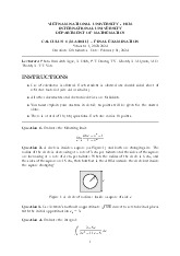
Đề thi cuối kỳ 2023 - 2024 môn Calculus 1 | Trường Đại học Quốc tế, Đại học Quốc gia Thành phố Hồ Chí Minh
35 18 -
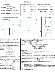
Note Calculus 1 Midterm - Calculus 1 | Trường Đại học Quốc tế, Đại học Quốc gia Thành phố HCM
660 330 -
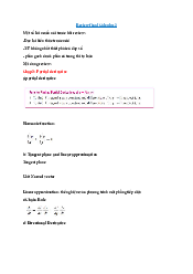
Review final Calculus - Calculus 1 | Trường Đại học Quốc tế, Đại học Quốc gia Thành phố HCM
437 219 -
Chapter 2 - Calculus 1 | Trường Đại học Quốc tế, Đại học Quốc gia Thành phố HCM
298 149