Chapter 8 Electronic stability control | Tài liệu môn Công nghệ kĩ thuật Ô tô Trường đại học sư phạm kỹ thuật TP. Hồ Chí Minh

Chapter 8
ELECTRONIC STABILITY CONTROL 8.1 INTRODUCTION 8.1.1
The functioning of a stability control system
Vehicle stability control systems that prevent vehicles from spinning and
drifting out have been developed and recently commercialized by several
automotive manufacturers. Such stability control systems are also often
referred to as yaw stability control systems or electronic stability control systems.
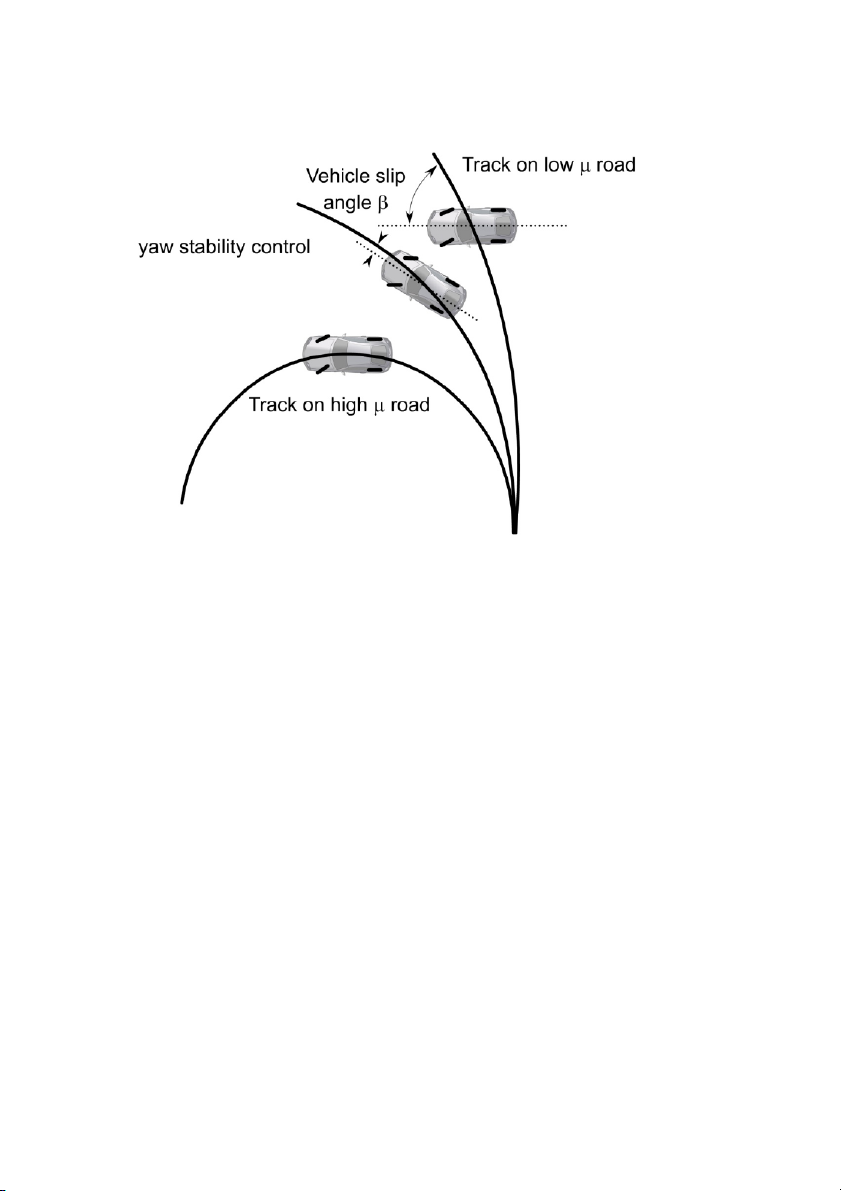
Figure 8-1 schematically shows the function of a yaw stability control
system. In this figure, the lower curve shows the trajectory that the vehicle
would follow in response to a steering input from the driver if the road were
dry and had a high tire-road friction coefficient. In this case the high friction
coefficient is able to provide the lateral force required by the vehicle to
negotiate the curved road. If the coefficient of friction were small or if the
vehicle speed were too high, then the vehicle would not follow the nominal
motion expected by the driver – it would instead travel on a trajectory of
larger radius (smaller curvature), as shown in the upper curve of Figure 8-1.
The function of the yaw control system is to restore the yaw velocity of the
vehicle as much as possible to the nominal motion expected by the driver. If
the friction coefficient is very small, it might not be possible to entirely achieve
the nominal yaw rate motion that would be achieved by the driver on a high
friction coefficient road surface. In this case, the yaw control system might
only partially succeed by making the vehicle’s yaw rate closer to the
expected nominal yaw rate, as shown by the middle curve in Figure 8-1.
R. Rajamani, Vehicle Dynamics and Control, Mechanical Engineering Series, 201
DOI 10.1007/978-1-4614-1433-9_8, © Rajesh Rajamani 2012 202 Chapter 8
Figure 8-1. The functioning of a yaw control system
The motivation for the development of yaw control systems comes from
the fact that the behavior of the vehicle at the limits of adhesion is quite
different from its nominal behavior. At the limits of adhesion, the slip angle is
high and the sensitivity of yaw moment to changes in steering angle becomes
highly reduced. At large slip angles, changing the steering angle produces
very little change in the yaw rate of the vehicle. This is very different from
the yaw rate behavior at low frequencies. On dry roads, vehicle maneuver-
ability is lost at vehicle slip angles greater than ten degrees, while on packed
snow, vehicle maneuverability is lost at slip angles as low as 4 degrees (Van Zanten, et. al., 1996).
Due to the above change of vehicle behavior, drivers find it difficult to
drive at the limits of physical adhesion between the tires and the road
(Forster, 1991, Van Zanten, et. al., 1996). First, the driver is often not able to
recognize the friction coefficient change and has no idea of the vehicle’s
stability margin. Further, if the limit of adhesion is reached and the vehicle
skids, the driver is caught by surprise and very often reacts in a wrong way
and usually steers too much. Third, due to other traffic on the road, it is
important to minimize the need for the driver to act thoughtfully. The yaw
control system addresses these issues by reducing the deviation of the
8. Electronic Stability Control 203
vehicle behavior from its normal behavior on dry roads and by preventing
the vehicle slip angle from becoming large. 8.1.2
Systems developed by automotive manufacturers
Many companies have investigated and developed yaw control systems
during the last ten years through simulations and on prototype experimental
vehicles. Some of these yaw control systems have also been commercialized
on production vehicles. Examples include the BMW DSC3 (Leffler, et. al.,
1998) and the Mercedes ESP, which were introduced in 1995, the Cadillac
Stabilitrak system (Jost, 1996) introduced in 1996 and the Chevrolet C5
Corvette Active Handling system in 1997 (Hoffman, et. al., 1998).
Automotive manufacturers have used a variety of different names for
yaw stability control systems. These names include VSA (vehicle stability
assist), VDC (vehicle dynamics control), VSC (vehicle stability control),
ESP (electronic stability program), ESC (electronic stability control) and DYC (direct yaw control). 8.1.3
Types of stability control systems
Three types of stability control systems have been proposed and developed for yaw control:
1) Differential Braking systems which utilize the ABS brake system on
the vehicle to apply differential braking between the right and left wheels to control yaw moment.
2) Steer-by-Wire systems which modify the driver’s steering angle input
and add a correction steering angle to the wheels
3) Active Torque Distribution systems which utilize active differentials
and all wheel drive technology to independently control the drive torque
distributed to each wheel and thus provide active control of both traction and yaw moment.
By large, the differential braking systems have received the most
attention from researchers and have been implemented on several production
vehicles. Steer-by-wire systems have received attention from academic
researchers (Ackermann, 1994, Ackermann, 1997). Active torque distribution
systems have received attention in the recent past and are likely to become
available on production cars in the future.
Differential braking systems are the major focus of coverage in this book.
They are discussed in section 8.2. Steer-by-wire systems are discussed in
section 8.3 and active torque distribution systems are discussed in section 8.4. 204 Chapter 8 8.2
DIFFERENTIAL BRAKING SYSTEMS
Differential braking systems typically utilize solenoid based hydraulic
modulators to change the brake pressures at the four wheels. Creating
differential braking by increasing the brake pressure at the left wheels
compared to the right wheels, a counter-clockwise yaw moment is generated.
Likewise, increasing the brake pressure at the right wheels compared to the
left wheels creates a clockwise yaw moment. The sensor set used by a
differential braking system typically consists of four wheel speeds, a yaw
rate sensor, a steering angle sensor, a lateral accelerometer and brake pressure sensors. 8.2.1 Vehicle model
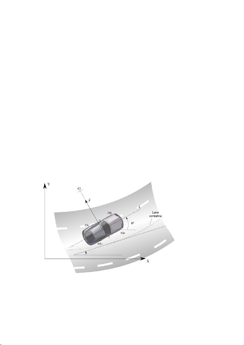
The vehicle model used to study a differential braking based yaw stability
control system will typically have seven degrees of freedom. The lateral and
longitudinal velocities of the vehicle ( x and y respectively) and the yaw
rate \ constitute three degrees of freedom related to the vehicle body. The
wheel velocities of the four wheels (Z Z Z Z f" , fr , r" and rr ) constitute the
other four degrees of freedom. Note that the first subscript in the symbols for
the wheel velocities is used to denote front or rear wheel and the second
subscript is used to denote left or right wheel. Figure 8-2 shows the seven
degrees of freedom of the vehicle model. \ des
Figure 8-2. Degrees of freedom for vehicle model for differential braking based system
8. Electronic Stability Control 205 Vehicle Body Equations
Let the front wheel steering angle be denoted by G . Let the longitudinal tire
forces at the front left, front right, rear left and rear right tires be given by x F " f , x F fr , x F r" and x
F rr respectively. Let the lateral forces at the front
left, front right, rear left and rear right tires be denoted by Fy "f , Fyfr , Fy " r
and F yrr respectively.
Then the equations of motion of the vehicle body are x m   F  F cos G ( )     sin(G )  \  xf" xfr  F F xr" xrr F F yf" yfr  m y (8.1) y m   F    sin G ( )   cos G ( )  \ " F   yr yrr F " F xf xfr  F " F yf yfr  m x (8.2) I \  "   "   "  z f  x F f" x F fr sin(G ) f  y F f" y F fr cos(G) r  y F r" y F rr " w   " " F  F "  F  F "  F "  F xfr cos(G ) w xf  xrr  w xr  yf yfr sin(G ) 2 2 2 (8.3) Here the lengths " " " f , r and
w refer to the longitudinal distance from
the c.g. to the front wheels, longitudinal distance from the c.g. to the rear
wheels and the lateral distance between left and right wheels (track width) respectively.
Slip Angle and Slip Ratio
Define the slip angles at the front and rear tires as follows y  "  \ f D G  f (8.4) x y "  \ r D   r (8.5) x
Define the longitudinal slip ratios at each of the 4 wheels using the following equations 206 Chapter 8 r Z  x eff w V x during braking (8.6) x r Z  x eff w V during acceleration (8.7) x r Z eff w
Let the slip ratios at the front left, front right, rear left and rear right be denoted by V V V V f" , fr , r" and rr respectively.
Combined Lateral-Longitudinal Tire Model Equations
The Dugoff tire model discussed in section 13.10 of this book can be utilized
for calculation of tire forces. Let the cornering stiffness of each tire be given
by C D and the longitudinal tire stiffness by V
C . Then the longitudinal tire
force of each tire is given by (Dugoff, et. al., 1969) V F C ( ) O (8.8) x V f 1 V
and the lateral tire force is given by tan(D ) F C (O ) y D f (8.9) 1 V where O is given by PF 1 (  V ) O z (8.10) 2 
^C V2 C tan(D)2 V D `1/2 and
f (O) (2  O )O if O  1 (8.11) f (O) 1 if O t 1 (8.12)
Fz is the vertical force on the tire while P is the tire-road friction coefficient.
8. Electronic Stability Control 207
Using equations (8.8), (8.9), (8.10), (8.11) and (8.12), the longitudinal
tire forces F x "f, x F fr , x F r" and F F , F ,
xrr and the lateral tire forces y " f yfr F y " r and y
F rr can be calculated. Note that the slip angle and slip ratio of
each corresponding wheel must be used in the calculation of the lateral and
longitudinal tire forces for that wheel. Wheel dynamics
The rotational dynamics of the 4 wheels are given by the following torque balance equations:  J Z   w " f d T "f b T "f e r ff Fx"f (8.13) J Z   w fr Tdfr b T fr e r ff Fxfr (8.14)  J Z   w " r d T " r b T " r e r ff x F " r (8.15) J Z   w rr Tdrr b T rr e r ff Fxrr (8.16) Here d T "
f , T dfr , d T r" and d
T rr refer to the drive torque transmitted to
the front left, front right, rear left and rear right wheels respectively and Tb "f, b T fr , b
T r" and T brr refer to the brake torque on the front left, front
right, rear left and rear right wheels respectively.
In general, the brake torque at each wheel is a function of the brake
pressure at that wheel, the brake area of the wheel w A , the brake friction
coefficient P b and the brake radius b
R . For instance, the brake torque at
the front left wheel Tb "f is related to the brake pressure at the front left
wheel P f" through the equation b T P f" w A b b R b P " f (8.17)
Similar equations can be written for the brake pressures b P fr , b P r" and b
P rr at the front right, rear left and rear right wheels respectively. 208 Chapter 8 8.2.2 Control architecture wheel speeds
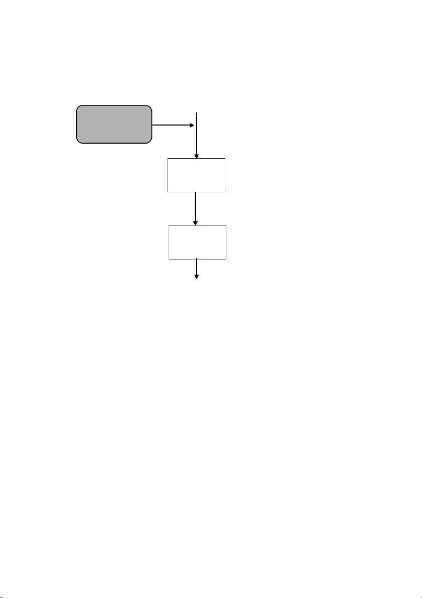
Objective: Yaw stability control lateral acceleration sensors yaw rate steering angle Upper Controller desired yaw torque Lower Controller Brake pressure inputs b P " , f P , P bfr b
P r" , brr
Figure 8-3. Structure of electronic stability control system
The control architecture for the yaw stability control system is hier-
archical and is shown in Figure 8-3. The upper controller has the objective of
ensuring yaw stability control and assumes that it can command any desired
value of yaw torque. It uses measurements from wheel speed sensors, a yaw
rate sensor, a lateral accelerometer and a steering angle sensor. Using these
measurements and a control law to be discussed in the following sub-
sections, it computes the desired value of yaw torque. The lower controller
ensures that the desired value of yaw torque commanded by the upper
controller is indeed obtained from the differential braking system. The lower
controller utilizes the wheel rotational dynamics and controls the braking
pressure at each of the 4 wheels to provide the desired yaw torque for the
vehicle. The inherent assumption is that the rotational wheel dynamics are
faster than the vehicle dynamics.
8. Electronic Stability Control 209 8.2.3 Desired yaw rate
In Chapter 3 (section 3.3), we saw that the steady state steering angle for
negotiating a circular road of radius R is given by "  " f r G  ss V K ay (8.18) R
where KV is the understeer gradient and is given by " m " m r K  V C 2 "  " C 2 "  " f D  f  f r D r f r where CD and C f r
D are the cornering stiffness for each front and rear tire respectively.
Hence, the steady state relation between steering angle and the radius of the vehicle’s trajectory is " "
§ m" C  m" C 2 · f r r r D f f D V G  ¨ ¸ (8.19) ss R
¨ 2C C ("  " ) ¸ R Df Dr f r © ¹
and the radius can be expressed in terms of steering angle as 1 G ss (8.20) R mV 2(" " ) r C r D f C f D "  "  f r 2C C L f D r D Here L "  " f
r is used to denote the wheelbase of the vehicle.
The desired yaw rate for the vehicle can therefore be obtained from
steering angle, vehicle speed and vehicle parameters as follows x x  \ G des (8.21) 2  "  " R x m ( ) r D C C r f Df "  "  f r 2 D C f D C L r 210 Chapter 8
Note that in the above equation, C C f D and r D stand for the cornering
stiffness of each front and rear tire and it is assumed that there are two tires
in the front and two tires in the rear. If the cornering stiffness of the front
and rear tires are equal, then C D C . f D C r D 8.2.4
Desired side-slip angle
In Chapter 3, we found that the steady state yaw angle error during cornering is " " 2 f " r mV e2 _    D ss (8.22) R C 2 "  r D  f " r  r r R R
and the steady state slip angle of the vehicle is E e 2 _ss or 2 " " f mV r E  (8.23) R C 2 " D  " r  f r  R
The above expression for steady state slip angle is in terms of velocity
and road radius. This expression can be rewritten so that the steady state slip
angle is expressed in terms of the steady state steering angle.
The steady –state steering angle, from equation (8.19) is "  " § m" C m" C 2 · f r r r D f D f V G ¨ ¸  ss R ¨ C 2 C ("  " ) ¸ R D f D r f r © ¹
Hence, the curvature of the road can be expressed as 1 Gss R mV 2 (" C  " C r D r f D f ) "  "  f r C 2 C L f D r D
8. Electronic Stability Control 211
Combining equations (8.23) and (8.20), the steady state slip angle is § " · 1 E ¨ f 2 ¨ "  mV r R 2C " " r D   f r  ¸ ¸ © ¹ or G § " · E ss ¨ f 2 " mV 2 ¨ r  mV (" C " " " r Dr  C ) 2C f Df D r   f r  ¸ ¸ © ¹ " f  " r  2C C L D f D r
which after simplification turns out to be 2 " f mV "  r 2CD "  " r  f r  E G des ss (8.24)  mV 2 " C  " C D D "  "  f r   r r f f  C 2 "  " f C D r D  f r 
Note: The above expression assumed that the cornering stiffness of each
front tire is C Df and of each rear tire is C r D .
Equation (8.24) describes the desired slip angle as a function of the
driver’s steering angle input, the vehicle’s longitudinal velocity and vehicle parameters. 8.2.5
Upper bounded values of target yaw rate and slip angle
The desired yaw rate and the desired slip angle described in sections 8.2.3
and 8.2.4 cannot always be obtained. It is not safe, for example, to try and
obtain the above desired yaw rate if the friction coefficient of the road is
unable to provide tire forces to support a high yaw rate. Hence the desired
yaw rate must be bounded by a function of the tire-road friction coefficient.
The lateral acceleration at the center of gravity (c.g.) of the vehicle is given by a x  \  y y _ cg (8.25) 212 Chapter 8
Since y x tan(E ) , the lateral acceleration can be related to the yaw
rate and the vehicle slip angle by the equation xE  a \ x  tan(E x y _ ) cg (8.26) 2 1  tan E
The lateral acceleration must be bounded by the tire-road friction coefficient P as follows a d Pg y _ cg (8.27)
The first term in the calculation of the lateral acceleration in equation
(8.26) dominates. If the slip angle of the vehicle and its derivative are both
assumed to be small, the second and third terms contribute only a small
fraction of the total lateral acceleration. Hence, combining equations (8.26)
and (8.27), the following upper bound can be used for the yaw rate Pg  \ 8 . 0 5 upper _ bound (8.28) x
The factor 0.85 allows the second and third terms of equation (8.26) to
contribute 15% to the total lateral acceleration.
The target yaw rate of the vehicle is therefore taken to be the nominal
desired yaw rate defined by equation (8.21) as long as it does not exceed the
upper bound defined by equation (8.28): \ \ \ d\ t ar e g t des if des upper _ bound (8.29) \ \ \ \ ! \ t arg et upperbound sgn( des ) if des upper _ bound (8.30)
The desired slip angle, for a given steering angle and vehicle speed, can
be obtained from equation (8.24). The target slip angle must again be upper
bounded so as to ensure that the slip angle does not become too large. At
high slip angles, the tires lose their linear behavior and approach the limit of
adhesion. Hence, it is important to limit the slip angle.
The following empirical relation on an upper bound for the slip angle is suggested
8. Electronic Stability Control 213 E  tan 1(0.02P ) upper _ g bound (8.31)
This relation yields an upper bound of 10 degrees at a friction coefficient
of P = 0.9 and an upper bound of 4 degrees at a friction coefficient of P =
0.35. This roughly corresponds to the desirable limits on slip angle on dry
road and on packed snow respectively.
The target slip angle of the vehicle is therefore taken to be the nominal
desired slip angle defined by equation (8.24) as long as it does not exceed
the upper bound defined by equation (8.31): E E E d E t arget des if (8.32) des upper _ bound E E sgn(E ) E ! E t arg et upperbound des if des upper _ bound (8.33)
Several researchers in literature have simply assumed the desired slip
angle to be zero and assumed that the upper bound on the yaw rate is given Pg by  \ upper _ bound
. However, the equations in (8.28) – (8.33) yield a x
better approximation to the driver-desired target values for both yaw rate and slip angle. 8.2.6
Upper controller design
The objective of the upper controller is to determine the desired yaw torque
for the vehicle so as to track the target yaw rate and target slip angle discussed in section 8.2.5.
The sliding mode control design methodology has been used by several
researchers to achieve the objectives of tracking yaw rate and slip angle
(Drakunov, et. al., 2000, Uematsu and Gerdes, 2002, Yi, et. al., 2003 and
Yoshioka, et. al., 1998). A good introduction to the general theory of sliding
surface control can be found in the text by Slotine and Li (1991).
The sliding surface is chosen so as to achieve either yaw rate tracking or
slip angle tracking or a combination of both. Examples of sliding surfaces
that have been used by researchers include the following three E s  [E (8.34) s \ \  targ et (8.35) 214 Chapter 8 s \ \  [E targ et (8.36)
By ensuring that the vehicle response converges to the surface s 0 ,
one ensures that the desired yaw rate and/or slip angle are obtained. A good
comparison of the performance obtained with the 3 types of sliding surfaces
described above can be found in Uematsu and Gerdes (2002).
This book suggests that the following sliding surface be used for control design: s \ \  [ E  E targ et  targ et  (8.37)
This surface is defined as a weighted combination of yaw rate and slip
angle errors and takes the target values for yaw rate and slip angle discussed
in sections 8.2.3 – 8.2.5 into consideration.
Differentiating equation (8.37) s \   \  [ E  E targ et  targ et  (8.38) The equation for \
 can be obtained by rewriting equation (8.3) as I \  " "   " "   " "  z f  x F f x F fr sin(G ) f  y F f y F fr cos(G) r  y F r y F rr " w    " " "   "  "  x F fr F cos(G ) w xf  x F rr F  w xr  yFf y F fr sin(G ) 2 2 2 (8.39) " Ignore the terms " w F "  yf F yfrsin(G) f  x F "  f Fxfr sin(G) and 2
in equation (8.39), assuming that the steering angle is small. Next, assume
that the ratio of front-to-back distribution of brake torques is fixed. Set x F U " r x F f" (8.40) and x F U rr Fxfr (8.41)
where U is determined by the front-to-back brake proportioning. The front-
to-back brake proportioning is determined by a pressure proportioning valve
8. Electronic Stability Control 215
in the hydraulic system. Many pressure proportioning valves provide equal
pressure to both front and rear brakes up to a certain pressure level, and then
subsequently reduce the rate of pressure increase to the rear brakes (see Gillespie, 1992).   I \ " F  F cos(G )  F  F z f  " yf yfr  " r " yr yrr  " (8.42) w   " w F  F cos(G )  U  " F F xfr xf   " xfr xf  2 2 Denote "w M \  b
Fxfr Fx"f  (8.43) 2 M b
\ is the yaw torque from differential braking and constitutes the
control input for the upper controller. Then \ 1 >" " "  cos G ( )  "   cos G ( )  U f F yf Fyfr  r F yr Fyrr   M\b@ Iz (8.44) Substituting for \  in equation (8.38) 1 s >"  cos( " G)  "   cos( " G)  U f  y F f y F fr  r  y F r y F rr   M b\ @ Iz \  [ E    E targ et  targ et  (8.45) Setting s K
 s yields the control law 216 Chapter 8 U  cos(G )M b \ I z ª " f " (8.46) « F "  G yf F cos( ) r yfr F "  yr y F rr  º » I I z z « « s K  \  [ E   E t ar e g t
  t ar egt  » » ¬ ¼
The control law described in equation (8.46) above requires feedback of
slip angle, slip angle derivative, and front and rear lateral tire forces. These
variables cannot be easily measured but must be estimated and used for
feedback. Estimation methods in literature use a combination of algorithms
based on integration of inertial sensors and dynamic model based observers
(Tseng, et. al., 1999, Van Zanten, et. al., 1996, Fukada, 1999, Ghoeneim,
2000, and Piyabongkarn, et. al., 2009). The use of GPS for estimation of slip
ratio and slip angle has also been investigated (Daily and Bevly, 2004, Bevly, et. al., 2001). " f " The term 
F "  F cos(G) F "  F yf  r yfr  yr yrr  in the upper I z I z
control law (8.46) is the yaw moment contribution due to lateral tire forces
(steering). In other words, the yaw moment contribution from lateral forces
is taken into account in determining the required yaw torque from
differential braking or other ESC system. The target yaw acceleration \  and  [(E  E )
t arg et is a feedforward term while the terms s K t arg et are feedback corrections. "
The lateral force yaw moment contribution 
f F "  F yf yfr cos(G )  Iz " r F
can be replaced in eqn (8.46) with an integral error feedback "  F yr yrr  Iz
term such as  ki ³s dt : U cosG M  K \  [ E    E b \ > k i s dt s ³ t arg ( ) et traget @ (8.47) Iz
This simplifies the measurement and estimation requirements for the
upper control law. However, control law (8.46) can provide better transient
8. Electronic Stability Control 217
performance than the simplified control law (8.47) based on the integral error feedback term. 8.2.7
Lower controller design
The lower controller determines the brake pressure at each wheel, so as to
provide a net yaw torque that tracks the desired value for yaw torque
determined by the upper controller. " By definition, w M 
. Hence, the extra differential b \ Fxfr Fx"f 2
longitudinal tire force needed to produce the desired yaw torque can be obtained as 2M b \ ' x F f (8.48) "w
Consider the dynamics of the front left and front right wheels  J Z  P  w f " Tdf" Aw b b R b P f" e r ff Fxf" (8.49) J Z  P  w fr Tdfr Aw b b R b P fr e r ff Fxfr (8.50)
The drive torque variables d T "
f and T dfr are determined by the driver
throttle input or by a combination of the driver throttle input and a traction
control system. The brake pressures b P " f and b
P fr are determined from the
braking input of the driver and the additional brake required to provide the
differential braking torque for vehicle yaw control.
By inspection of equations (8.49) and (8.50), it can be seen that the
desired differential longitudinal tire force F
' xf at the front tires can be
obtained by choosing the brake pressures at the front left and right tires as follows: F ' xf reff "  b P f P0 a (8.51) A P w b Rb F ' xf erff P P  1 (  a) bfr 0 (8.52) A P w bRb 218 Chapter 8 where 0
P is the measured brake pressure at the wheel at the time that
differential braking is first initiated and the constant a has to be chosen such
that 0 d a d 1 and b P " f and b
P fr are both positive. The brake pressure at
each wheel should be zero or positive. Hence, in the case where the driver is not braking, P x F ' f is positive, and 0 0
, then a has to be chosen to be
zero. On the other hand, if the driver is braking and 0
P is adequately large,
then a could be chosen to be 0.5. This would mean that the differential
braking torque is obtained by increasing the brake pressure at one wheel and
decreasing the brake pressure at the other wheel compared to the driver
applied values. Thus a must be chosen in real-time based on the measured value of 0 P . 8.3 STEER-BY-WIRE SYSTEMS 8.3.1 Introduction
In the use of a steer-by-wire system for yaw stability control, the front wheel
steering angle is determined as a sum of two components. One component is
determined directly by the driver from his/her steering wheel angle input.
The other component is decided by the steer-by-wire controller, as shown in
Figure 8-4. In other words, the steer-by-wire controller modifies the driver’s
steering command so as to ensure “skid prevention” or “skid control”. This
must be done in such a way that it does not interfere with the vehicle’s
response in following the path desired by the driver.
Significant work on the design of steer-by-wire systems for vehicle
stability control has been documented by Ackermann and co-workers
(Ackermann, 1997, Ackermann, 1994). The following sub-sections summarize
the steer-by-wire control system for front-wheel steered vehicles designed by Ackermann (1997).
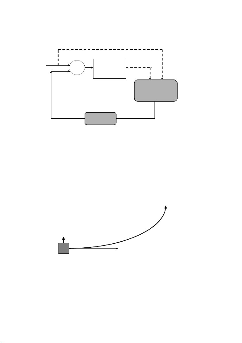
8. Electronic Stability Control 219 Gdriver Driver Vehicle + Dynamics Gsbw wheel speeds lateral acceleration yaw rate steering angle sensors Steer by wire controller
Figure 8-4. Structure of steer-by-wire stability control system 8.3.2
Choice of output for decoupling
As described in Ackermann (1997), the driver’s primary task is “path
following”. In path following the driver keeps the car – considered as a
single point mass m - on her desired path, as shown in Figure 8-5. She does
this by applying a desired lateral acceleration a yP to the mass m in order to
re-orient the velocity vector of the vehicle so that it remains tangential to her desired path. desired path a yP velocity point mass
Figure 8-5. The path following task of the driver 220 Chapter 8
The driver has a secondary task of “disturbance attenuation.” This task
results from the fact that the vehicle is not really a point mass but has a
second degree of freedom which is the yaw motion of the vehicle. Let the
yaw moment of inertia of the vehicle be I . The yaw rate of the car is z
excited not only by the driver desired lateral acceleration a yP but also by a
disturbance torque M zD. The yaw rate excited by the lateral acceleration a
is expected by the driver and she is used to this yaw rate. However, yP
disturbances such as a flat tire and asymmetric friction coefficients at the left
and right wheels induce a disturbance torque M which excite a yaw zD
motion that the driver does not expect.
Usually, the driver has to compensate for the disturbance torque by using
the steering wheel. This is a difficult task for the driver due to the fact that
she is not used to counteracting for such disturbances and also due to the fact
that she does not have a measure of the disturbances that cause the
unexpected yaw and therefore her reaction is likely to be delayed. It often
takes time for the driver to recognize the situation and the need for her special intervention.
In Ackermann (1997), the steer-by-wire electronic stability control
(ESC) system is designed to perform this task of disturbance attenuation so
that the driver can concentrate on her primary task of path following. For
this it is necessary to decouple the secondary disturbance attenuation
dynamics such that they do not influence the primary path following
dynamics. The automatic control system for the yaw rate \ should not
interfere with the path following task of the driver. In control system terms,
this means the yaw rate \ should be unobservable from the lateral accele-
ration a yP. The yaw rate dynamics will continue to depend on the lateral
acceleration a yP. Only then can the driver control the car to follow a path,
since the vehicle must have a yaw rate to follow a path. However, the yaw
rate is commanded only indirectly by the driver via a yP . Nominally the
driver is concerned directly only with a yP . But any yaw rate induced by the
disturbance attenuation automatic steering control system should be such
that it does not affect the lateral acceleration a yP . This decoupling has to be
done in a robust manner. In particular, it must be robust with respect to
vehicle velocity and road surface conditions.
From the above discussion, the motivation for removing the influence of
yaw rate on lateral acceleration is clear. The next question to be answered is
“At which point of the vehicle should the lateral acceleration be used as the
output ?” The lateral acceleration at any point P on the vehicle is given by