Homework Review: Key Concepts in Volatility and Risk Management | Môn Derivatives and Risk Management - Trường Đại học Quốc tế, Đại học Quốc gia Thành phố Hồ Chí Minh

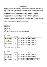
lOMoAR cPSD| 23136115 CHAP 10: VOLATILITY
10.1 The volatility of an asset is 2% per day. What is the standard deviation of the
percentage price change in three days?
⇨ Standard deviation: 2% x √ ❑ = 3.46%
10.2 The volatility of an asset is 25% per annum. What is the standard deviation of the percentage price
change in one trading day? Assuming a normal distribution with zero mean, estimate 95% confidence
limits for the percentage price change in one day. ⇨ Standard deviation: = 1.57% ❑ Confidence limits: 25 x x 1.96 = +/- 3.09% ❑
10.3 Why do traders assume 252 rather than 365 days in a year when using volatilities?
⇨ Volatility is much higher when markets are open than when they are closed. Traders, therefore, measure
time in trading days rather than calendar days.
Or: When markets are open compared to when they are closed, volatility is significantly higher. So instead
of using calendar days to measure time, traders use trading days.
10.4 What is implied volatility? What does it mean if different options on the same asset have different implied volatilities?
⇨Implied volatility is the real-time estimation of an asset's price as it trades. Implied volatility tends to
increase when options markets experience a downtrend. Implied volatility falls when the options market
shows an upward trend. Larger implied volatility means higher options prices.
⇨The implied volatility for puts and calls and for options contracts with different strike prices or expiration
dates that are all based on the same underlying asset will have different implied volatilities because the
different options will each have a different supply-demand equilibrium.
10.5 Suppose that observations on an exchange rate at the end of the past 11 days have been 0.7000,
0.7010, 0.7070, 0.6999, 0.6970, 0.7003, 0.6951, 0.6953, 0.6934, 0.6923, and 0.6922. Estimate the daily
volatility using both equations (10.2) and equation (10.4).
⇨ Standard deviation gives 0.547
10.6 The number of visitors to websites follows the power law in equation (10.1) with α = 2. Suppose that
1% of sites get 500 or more visitors per day. What percentage of sites get (a) 1,000 and (b) 2,000 or more visitors per day?
⇨ The power law: 0.01 = K x 500−2 ⇔ K = 2500
a. Percentage of sites get 1000: 2500 x 1000−2 = 0.0025 = 0.25%
b. Percentage of sites that get 2000 or more visitors per day: 2500 x 2000−2 = 0.000625 = 0.0625% lOMoAR cPSD| 23136115
10.9 The most recent estimate of the daily volatility of an asset is 1.5% and the price of the asset at the
close of trading yesterday was $30.00. The parameter λ in the EWMA model is 0.94. Suppose that the
asset's price at the close of trading today is $30.50. How will this cause the volatility to be updated by the EWMA Model?
⇨, In this case, σ n−1 = 0.015
σ 2n = 0.94 x 0.0152 + 0.06 x 0.01672 = 0.0002282
The volatility estimate on day n is, therefore: √❑ = 0.0151 or 1.51%
10.11 Assume that an index at the close of trading yesterday was 1,040 and the daily volatility of the
index was estimated as 1% per day at that time. The parameters in a GARCH(1,1) model are ω =
0.000002, α = 0.06, and β = 0.92. If the level of the index at the close of trading today is 1,060, what is the new volatility estimate? ⇨ With the usual notation:
σ 2n = 0.000002 + 0.06 x 0.019232 + 0.92 x 0.012= 0.0001162
The volatility estimate on day n is, therefore: σ n = √❑ = 0.01078 or 1.078% per day
10.12 The most recent estimate of the daily volatility of the dollar–sterling exchange rate is 0.6%. The
exchange rate at 4:00 p.m. yesterday was 1.5000. The parameter λ in the EWMA model is 0.9. Suppose
that the exchange rate at 4:00 p.m. today proves to be 1.4950. How would the estimate of the daily volatility be updated?
⇨ The proportional daily change is = -0.0033
The current daily variance estimate is 0.0062 = 0.000036
The new daily variance estimate is 0.9 x 0.000036 + 0.1 x 0.00332 = 0.0000335
The new volatility is the square root of this: √❑ = 0.00579 = 0.579%
10.14 The parameters of a GARCH(1,1) model are estimated as ω = 0.000004, α = 0.05, and β = 0.92. What
is the long-run average volatility and what is the equation describing how the variance rate reverts to its
long-run average? If the current volatility is 20% per year, what is the expected volatility in 20 days? ω
⇨ The long-run average variance: V L = 1− α−β = = 0.000133
The long-run average volatility is √❑ = 0.012 = 1.2% per day σ n = 0.2 = 0.0126 √❑ lOMoAR cPSD| 23136115
The expected variance in 30 days: 0.000133 + 0.9720 (0.01262 - 0.000133) = 0.000147
The expected volatility per day is, therefore: √❑ = 0.0121 or 1.21%
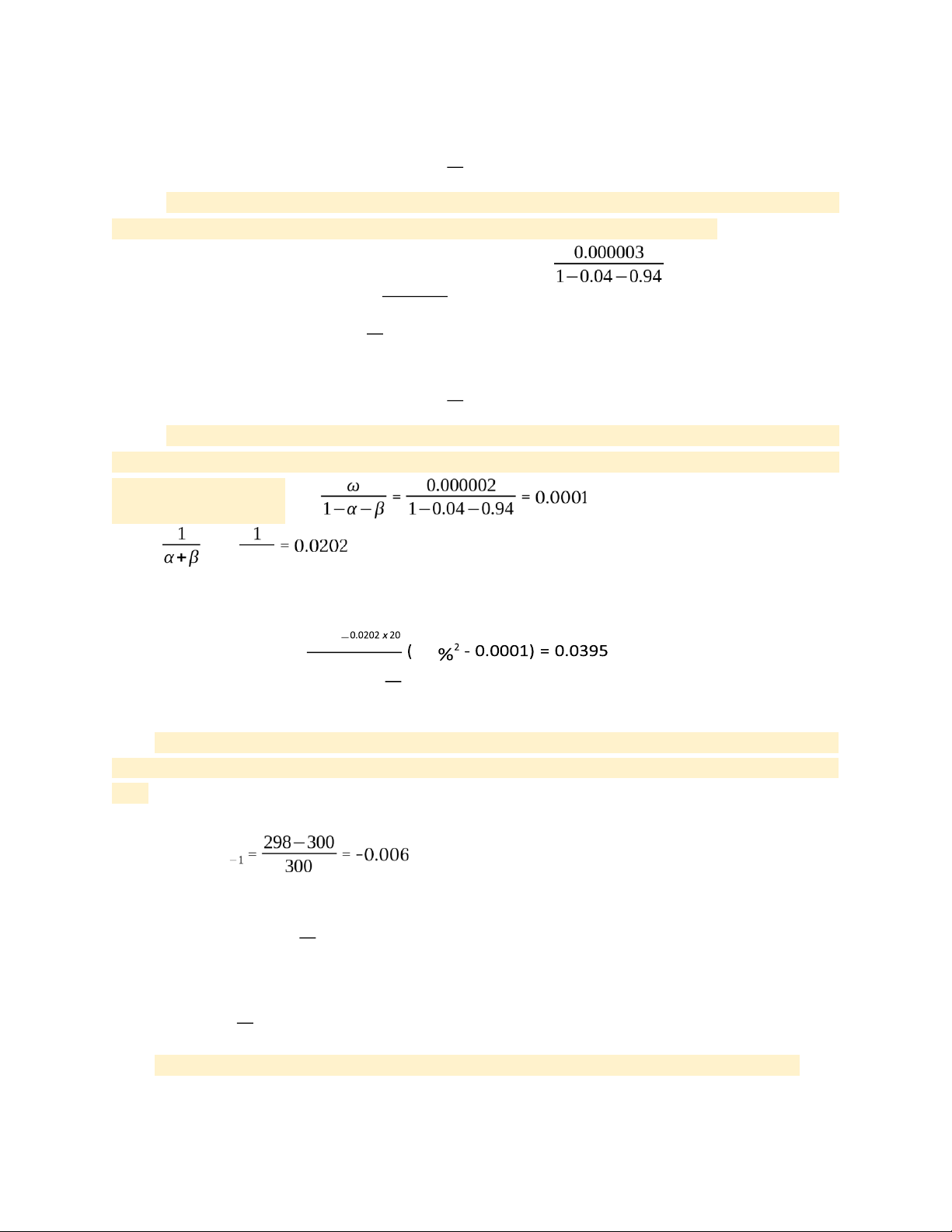
10.16 Suppose that GARCH(1,1) parameters have been estimated as ω = 0.000003,α = 0.04, and β = 0.94.
The current daily volatility is estimated to be 1%. Estimate the daily volatility in 30 days. ω
⇨ The long-run average variance: V L = 1−α−β = = 0.00015
The long-run average volatility is √❑ = 0.0122 = 1.22% per day
The expected variance in 30 days: 0.00015 + 0.9830 (0.012 - 0.00015) = 0.000123
The expected volatility per day is, therefore: √❑ = 0.011 or 1.1%
10.17 Suppose that GARCH(1,1) parameters have been estimated as ω = 0.000002,α = 0.04, and β = 0.94.
The current daily volatility is estimated to be 1.3%. Estimate the volatility per annum that should be used
to price a 20-day option. V L = α = ln = ln 0.98
σ(20)2 = 252 x ( 0.0001 + 1−e 1.3 0.0202x20
The volatility per annum: σ(20) = √❑ = 0.1987 = 19.87%
10.19 Suppose that the price of an asset at the close of trading yesterday was $300 and its volatility was
estimated as 1.3% per day. The price at the close of trading today is $298. Update the volatility estimate using
(a) The EWMA model with λ = 0.94
σ t−1 = 0013 Rt
EWMA: σ 2n = 0.94 x 0.132 + (1-0.94) x 0.0062= 0.00016
The new daily volatility is √ ❑ = 0.12 = 1.2%
(b) The GARCH(1,1) model with ω = 0.000002, α = 0.04, and β = 0.94.
GARCH(1,1) = 0.000002 x 0.04 x 0.0062 x 0.94 x 0.00132 = 0.00016 The new
daily volatility is √ ❑ = 0.12 = 1.2%
10.21 Suppose that the parameters in a GARCH(1,1) model are α = 0.03,β = 0.95, and ω = 0.000002.
(a) What is the long-run average volatility? lOMoAR cPSD| 23136115 V L =
The long-run average volatility is √❑ = 0.01
(b) If the current volatility is 1.5% per day, what is your estimate of the volatility in 20, 40, and 60 days? σ n = 1.5% ● t=20 days
E [σ 2n+20 ] = 0.0001 + (0.03+0.95)20 (1.5%2 - 0.0001) = 0.000183
Expected volatility in 20 days = √❑ = 0.0135 = 1.35% ● t=40 days
E [σ 2n+40 ] = 0.0001 + (0.03+0.95)40 (1.5%2 - 0.0001) = 0.0001557
Expected volatility in 40 days = √❑ = 0.0125 = 1.25% ● t=60 days
E [σ 2n+60 ] = 0.0001 + (0.03+0.95)60 (1.5%2 - 0.0001) = 0.000137 Expected
volatility in 60 days = √❑ = 0.0117 = 1.17%
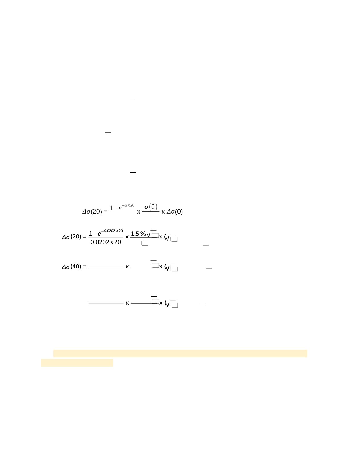
(c) What volatility should be used to price 20-, 40-, and 60-day options?
−α T σ(T)2 = 252 x 1−e ( V L +
( V 0 - V L )) αT❑ α = ln = ln = 0.0202 0.03 ● t=20 days
−0.0202x 20 σ(20)2 = 252 x ( 0.0001 +
1−e (1.5%2 - 0.0001) = 0.051 0.0202x20 = 0.226 = 22.6% ● t=40 days
−0.0202x 40 σ(40)2 = 252 x ( 0.0001 +
1−e (1.5%2 - 0.0001) = 0.0468 0.0202 x 40 = 0.2164 = 21.64% ● t=60 days
−0.0202x 60 σ(60)2 = 252 x ( 0.0001 +
1−e (1.5%2 - 0.0001) = 0.04346 0.0202x60 = 0.2085 = 20.85% lOMoAR cPSD| 23136115
(d) Suppose that there is an event that increases the volatility from 1.5% per day to 2% per
day. Estimate the effect on the volatility in 20, 40, and 60 days. σ n = 2% = 0.02 ● t=20 days
E [σ 2n+20 ] = 0.0001 + 0.9820 (0.022 - 0.0001) = 0.0003
Expected volatility in 20 days = √❑ = 1.73% ● t=40 days
E [σ 2n+40 ] = 0.0001 + 0.9840 (0.022 - 0.0001) = 0.000233 Expected
volatility in 20 days = √❑ = 1.53% ● t=60 days
E [σ 2n+60 ] = 0.0001 + 0.9860 (0.022 - 0.0001) = 0.000189
Expected volatility in 60 days = √❑ =1.38%
(e) Estimate by how much the event increases the volatilities used to price 20-, 40-, and 60- day options. ● t=20 → α x20 σ(20)
x 2% - √❑ x 1.5%) = 0.0688 = 6.88% ● t=40
1−e−0.0202x 40 1.5%√
x 2% - √❑ x 1.5%) = 0.0599 = 5.99% 0.0202 x 40 ❑ ● t=60
Δσ(60) = 1−e−0.0202x 60 1.5%√
x 2% - √ ❑ x 1.5%) = 0.0525 = 5.25% 0.0202x60 ❑ CHAP 12
12.1 What is the difference between expected shortfall and VaR? What is the theoretical advantage of the expected shortfall over VaR?
VaR gives the Xth quantile a 100% weighting and the other quantiles a 0% value. All quantiles
above the Xth quantile are given equal weight by the expected shortfall, whereas all quantiles
below the Xth quantile are given zero weight. lOMoAR cPSD| 23136115
12.3 A fund manager announces that the fund’s one-month 95% VaR is 6% of the size
of the portfolio being managed. You have an investment of $100,000 in the fund. How do you interpret
the portfolio manager’s announcement? -
It has been interpreted that a 5% chance of a loss of 6000 (100,000 x 6%) occurs on such investment in a portfolio
You can see how the VaR question has 3 elements: a relatively high level of confidence (95%), a time
period (a month) and an estimate of investment loss (6% or 6000) -
Then is 6% chance that you will lose at least 0.06 x 100,000 = $6,000 over a onemonth period 12.4
A fund manager announces that the fund’s one-month 95% expected shortfall is 6% of the size of
the portfolio being managed. You have an investment of $100,000 in the fund. How do you interpret the
portfolio manager’s announcement?
You anticipate losing $6,000 in a poor month. Bad months are those that have returns that are below the
five-percentile point on the monthly return distribution. 12.5
Suppose that each of the two investments has a 0.9% chance of a loss of $10 million and a 99.1%
chance of a loss of $1 million. The investments are independent of each other.
(a) What is the VaR for one of the investments when the confidence level is 99%?
The VaR for one of the investments when the confidence level is 99% is $1 million.
(b) What is the expected shortfall for one of the investments when the confidencelevel is 99%?
When the confidence level is 99%
Out of the remaining 1%: 0.1% has a chance of a loss of $1 million and 0.9% has a chance of a loss of $10 million.
This implied there is a 10% chance of a loss of $1 million and a 90% chance of a loss of $10 million.
So, the expected shortfall for one of the investments is:
0.1 x $1 million + 0.9 x $10 million = $9.1 million
(c) What is the VaR for a portfolio consisting of two investments when theconfidence level is 99%?
There is 0.009 x 0.009 = 0.000081 probability of loss $20 million ($10 million + $10 million)
There is 2 x 0.009 x 0.991 = 0.017838 probability of loss $11 million ($10 million + $1 million)
There is 0.991 x 0.991 = 0.982081 probability of loss $2 million ($1 million + $1 million) Since 0.017838 + 0.982081 = 0.999919
→ If the confidence level is 99% then the VaR for a portfolio consisting of the two investment is $11 million lOMoAR cPSD| 23136115
(d) What is the expected shortfall for a portfolio consisting of the two investmentswhen
the confidence level is 99%?
When the confidence level is 99%, the remaining tail of the distribution is 1% or 0.01
0.000081 / 0.01 = 0.0081 probability of loss of $20 million
1- 0.0081 = 0.9919 probability of loss of $11 million
The expected shortfall for the portfolio for 2 investments
0.0081 x $20 million + 0.9919 x $11 million = $11.0729 million
(e) Show that in this example VaR does not satisfy the subadditivity condition, whereas
expected shortfall does.
The sum of the VaR of the investments separately = $ (1+1) million = $2 million
As, the VaR of the portfolio of the two investments is greater than the sum of the VaR of the investment
separately, this does not satisfy the subadditivity condition. Sum of shortfall of the investment separately
= $ (9.1 + 9.1) million = $18.2 million Shortfalls of the portfolio of the two investments = $11.0729 million
As, shortfalls of the portfolio of the two investments are less than the sum of shortfalls of the investments
separately, satisfies subadditivity condition
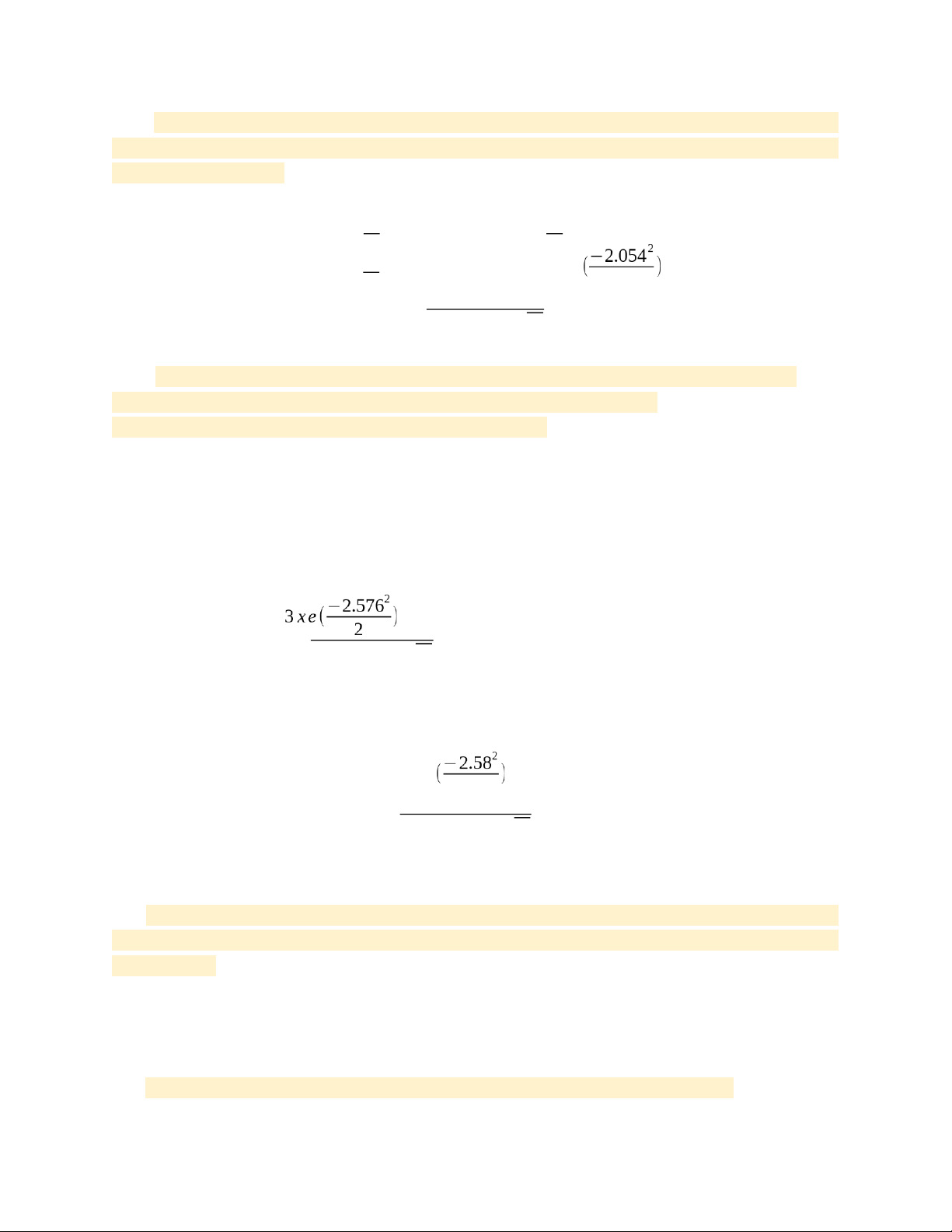
12.6 Suppose that the change in the value of a portfolio over a one-day time period is normal with a mean
of zero and a standard deviation of $2 million; what is (a) the one-day 97.5% VaR, (b) the five-day 97.5%
VaR, and (c) the five-day 99% VaR? - Option 1:
The formula: normal distribution value x daily VaR x (days)0.5
a. 97.5% VaR, here 1.96 as per normal distribution table: 1.96 x $2 million = 3919927,97
b. 5 days - 97.5% VaR: 1.96 x 2 x 106 x 50.5 = 8765225,41
c. 5 days - 99% VaR: 2.326 x 2 x 106 x 50.5 = 10403743,97 - Option 2:
a. 1 day 97.5% VaR = 0 + 2 x N−1(0.975) = 0 + 2 x 1.96 =
b. 5 days 97.5% VaR = √❑ x 2 x 1.96 = $8.7 million
c. 5 days 99% VaR = √❑ x 2 x N−1(0.99) = √❑ x 2 x 2.33 = $1-.4 million
12.7 What difference does it make to your answer to Problem 12.6 if there is first-order daily
autocorrelation with a correlation parameter equal to 0.16?
12.9 Suppose that we back-test a VaR model using 1,000 days of data. The VaR confidence level is 99% and
we observe 17 exceptions. Should we reject the model at the 5% confidence level? Use a one-tailed test.
The probability of the VaR being exceeded on a given day P = 1 - 0.99 = 0.01
The probability of the VaR being exceeded on 17 days or more:
1 - Biodist (16,10000; 0.01; True) = 2.64% < 5% → The model should be accepted lOMoAR cPSD| 23136115
12.12 The change in the value of a portfolio in one month is normally distributed with a mean of zero and
a standard deviation of $2 million. Calculate the VaR and ES for a confidence level of 98% and a time horizon of three months.
● 3 months 98% VaR = 0 + √❑ x 2 x N−1(0.98) =0 + √❑ x 2 x 2.054 = $7.11 million e
● 3 months 98% ES = 0 + √❑ x 2 x 2 = $8.38 million (1−98%)x√❑
12.16 The change in the value of a portfolio in three months is normally distributed with a mean of
$500,000 and a standard deviation of $3 million. Calculate the VaR and ES for a
confidence level of 99.5% and a time horizon of three months. - Option 1:
The loss has a standard deviation of 3000 and a mean of -500
Mean = $500,000 = $0.5 million
Standard Derivation = $3 million
Z - coefficient at 99.5% probability = 2.5759
VaR = Mean - z - coefficient x ST = 0.5 - 2.5759 X 3 = -7,227 million
→ Value at risk= $7,227 million Expected Shortfall: 0.5 + = $8.176 million (1−0.995)x√❑ - Option 2:
● 3 months 99.5% VaR = 0.5 + 3 x N−1(0.995) =0 + 3 x 2.58 = $8.24 million e
● 3 months 99.5% ES = 0 + 3 x 2 = $9.08 million (1−99.5%)x√❑ CHAP 15
15.1 “When a steel company goes bankrupt, other companies in the same industry benefit because they
have one less competitor. But when a bank goes bankrupt other banks do not necessarily benefit.” Explain this statement.
The removal of a competitor may be beneficial. However, banks enter into many contracts with each other.
When one bank goes bankrupt, others banks will be adversely affected if the bankruptcy reduces the
public’s overall level of confidence in the banking system.
15.5 A four-year interest rate swap currently has a negative value to a financial institution. lOMoAR cPSD| 23136115
Is the financial institution exposed to credit risk on the transaction? Explain your answer. How would the
capital requirement be calculated under Basel I?
There is some exposure. If the counterparty defaulted now three would be no loss. However, inter rates
could change so that at a future time the swap has a positive value to financial institutions. The capital
under Basel I would, from table 15.2, be 0.5% of the swap’s principal.
15.6 Estimate the capital required under Basel I for a bank that has the following transactions with a
corporation. Assume no netting. (a)
A nine-year interest rate swap with a notional principal of $250 million and a current market value of −$2 million.
● Credit equivalent amount = 250 x 1.5% = $3.75 million
● Risk-weighted assets = 3.75 x 0.5 = $1,875 million (b)
A four-year interest rate swap with a notional principal of $100 million and a currentvalue of $3.5 million.
● Credit equivalent amount = 100 x 0.5% + 3.5 = $4 million
● Risk-weighted assets = 4 x 0.5 = $2 million (c)
A six-month derivative on a commodity with a principal of $50 million that is currentlyworth $1 million.
● Credit equivalent amount = 550 x 10% + 1 = $6 million
● Risk-weighted assets = 6 x 0.5 = $3 million
→ Total capital required = 8% (1,875 + 2 + 3) = $0.55 million
15.7 What is the capital required in Problem 15.6 under Basel I assuming that the 1995 netting amendment applies?
The current exposure with netting: -2 + 3.5 + 1 = 2.5
The current exposure without netting: 3.5 + 1 = 4.5 2.5 NRR = = 0.556 4.5
The credit equivalent amount: 2.5 + (0.4 + 0.6 x 0.556) x 9.25 = 9.28
The risk-weight assets are: 9.28 x 0.5 = 4.64
The capital required is: 4.64 x 0.08 = 0.3712
15.13 Equation (15.9) gives the formula for the capital required under Basel II. It involves four terms being
multiplied together. Explain each of these terms. 12.5 x EAD x LGD x (WCDR -PD)
● EAD is the estimated exposure at default lOMoAR cPSD| 23136115
● LGD is the loss given default, which is the proportion of the exposure that will be a loss if a default occurs
● WCDR is the one-year probability of default in a bad year that occurs only one time in 1000
● PD is the probability of default in an average year
● MA is the maturity adjustment, which allows for the fact that, in the case of instruments lasting
longer than a year, there may be losses arising from a decline in the creditworthiness of the
counterparty during the tear as well as from default during the year.
15.17 Suppose that the assets of a bank consist of $200 million of retail loans (not mortgages). The PD is
1% and the LGD is 70%. What are the risk-weighted assets under the Basel II IRB approach? What are the
Tier 1 and Tier 2 capital requirements?
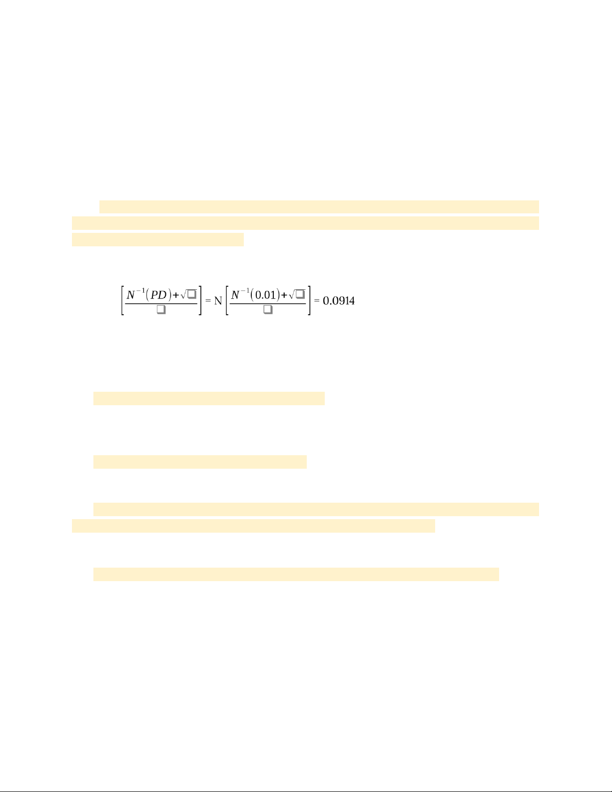
For retail exposure: p = 0.03 + 0.13 e−35xPD = 0.03 + 0.13 e−35x 0.01 = 0.1216 WCDR = N
The capital requirement: 200 x 0.7 x (0.0914 - 0.01) = $11.39 million
→ At least half of this must be Tier 1 CHAP 16
16.1 What are the three major components of Basel II.5?
The three major components of Basel II.5 are the calculation of screeded VaR and a new incremental risk
charge. And a comprehensive risk measure for instruments dependent on credit correlation.
16.2 What are the six major components of Basel III?
The six major components of Basel III are capital definitions and requirements, the capital conservation
buffer, the countercyclical buffer, the leverage ratio, liquidity ratios, and counterparty credit risk.
16.6 By how much has the Tier 1 equity capital (including the capital conservation buffer) increased under
Basel III compared with the Tier 1 equity capital requirement under Basel I and II?
Tier 1 equity capital has increased from 2% to 7%, and the definition of equity capital has been tightened.
16.8 Explain how the leverage ratio differs from the usual capital ratios calculated by Regulators.
In the leverage ratio, the denominator is not risk-weighted assets. It is total assets on the balance sheet
without risk-weighting plus derivatives exposures (calculated as in Basel I) and some off-balance sheet items such as loan commitment
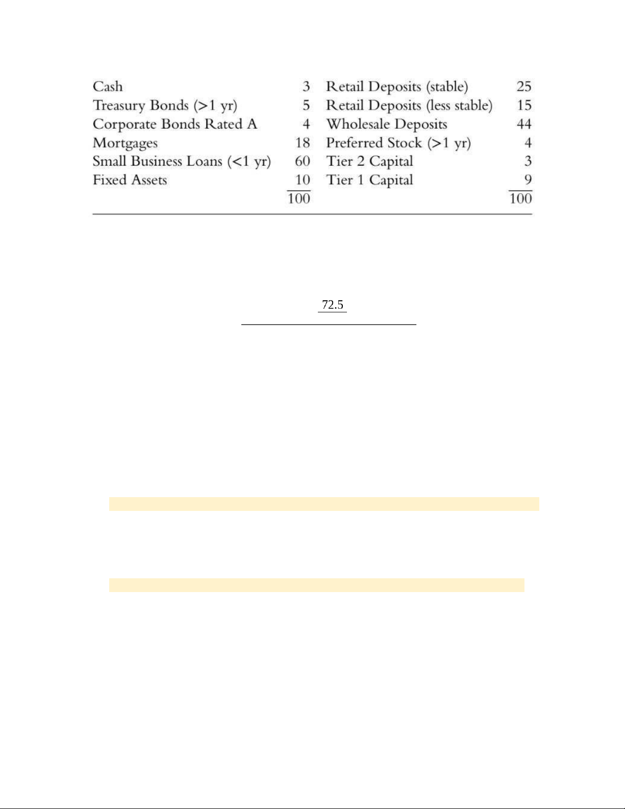
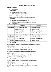
16.14 A bank has the following balance sheet: lOMoAR cPSD| 23136115
(a) What is the Net Stable Funding Ratio?
● Amount of Stable Funding: 25 x 90% + 15 x 80% + 44 x 50% + 4 x 1 + 3 x 1 + 9 x 1 = 72.5 ● Required amount of Stable Funding:
3 x 0% + 5 x 5% + 4 x 50% + 18 x 65% + 60 x 85% + 10 x 1 = 74.95
→ NSFR (Net Stable Funding Ratio) =
Required amountof Stable
FundingAmount of StableFunding = 74.95 = 0.967 or 96.7%
So, the bank doesn’t satisfy NSFR requirement
(b) The bank decides to satisfy Basel III by raising more (stable) retail deposits andkeeping the
proceeds in Treasury bonds. What extra retail deposits need to be Raised?
● Call y as the extra amount of retail deposits
● We have: 0.9y + 72.5 = 0.05y + 74.95 → y = 2.882 CHAP 19: 19.1
How many different ratings does Moody’s use for investment-grade companies? What are they?
According to Moody, they use 10 different ratings for investment-grade companies: Aaa, Aa1, Aa2, Aa3,
A1, A2, A3, Baa1, Baa2, and Baa3. 19.2
How many different ratings does S&P use for investment-grade companies? What are they?
S&P used for investment-grade companies is AAA, AA+, AA. AA-, A+, A, A-, BBB+, BBB, BBB- lOMoAR cPSD| 23136115 19.3
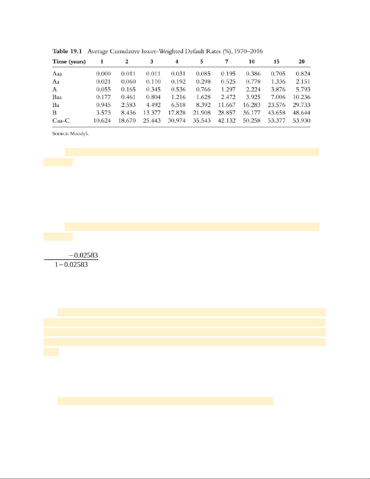
Calculate the average hazard rate for a B-rated company during the first year from the data in Table 19.1.
Q(t) = 1 - e−λ(t)t = 3.573%
→ e−λx1 = 1 - 0.03573
→ λ = -ln (0.96427) = 0.0364 = 3.64% 19.4
Calculate the average hazard rate for a Ba-rated company during the third year from the data in Table 19.1.
● Conditional on no default by year 2, the prob. Of a default in year 3: 0.04492 = 0.0196
● Average hazard rate for the third year: e−λ x1 = 1 -
0.0196 → λ = -ln (0.9804) =1.98%
19.5 A credit default swap requires a semiannual payment at the rate of 60 basis points per year. The
principal is $300 million and the credit default swap is settled in cash. A default occurs after four years and
two months, and the calculation agent estimates that the price of the cheapest deliverable bond is 40% of
its face value shortly after the default. List the cash flows and their timing for the seller of the credit default swap.
The seller receives their payment from the buyer at the times 0.5, 1, 1.5, 2.0, 2.5, 3.0, 3.5 and 4 years:
300,000,000 x 0.006 x 0.5 = $900,000 The seller pays the payoff of the CDs:
Payoff = (1 - 40%) x 300,000,000 = $180,000,000
19.7 Explain the difference between risk-neutral and real-world default probabilities. Risk-neutral default
prob. are backed out from credit spreads. Real-world default prob. Are calculated from historical data.
Risk-neutral default prob should be used for valuation. Real-world default prob. Should be used for
scenario analysis and credit VaR calculations. lOMoAR cPSD| 23136115
19.8 What is the formula relating the payoff on a CDS to the notional principal and the recovery rate?
The payoff is L(1-R) where L is the notional principal and R is the recovery rate
19.9 The spread between the yield on a three-year corporate bond and the yield on a similar risk-free bond
is 50 basis points. The recovery rate is 30%. Estimate the average hazard rate per year over the three-year period.
From equation (19.3) the average hazard rate over the three years is 0.005 (1 - 0.3) = 0.0071 or 1%
19.11 Should researchers use real-world or risk-neutral default probabilities for (a) calculating credit value
at risk and (b) adjusting the price of a derivative for default? The real-world prob of default should be used
for calculating credit value at risk. Riskneutral prob of default should be used for adjusting the price of a derivative for default.
19.18 The value of a company’s equity is $2 million and the volatility of its equity is 50%. The debt that will
have to be repaid in one year is $5 million. The risk-free interest rate is 4% per annum. Use Merton’s model
to estimate the probability of default. (Hint: The Solver function in Excel can be used for this question.)
In this case P0 = 2, σ E = 0.5, D = 5, r = 0.04
Solving the simultaneous equation give V 0 = 6.0 and σ V = 14.82
The prob of default is N (-d2) or 1.15%