Jet trajectory and flow through an orifice | Môn Fluid Mechanics Lab - Trường Đại học Quốc tế, Đại học Quốc gia Thành phố Hồ Chí Minh

lOMoAR cPSD| 58583460
Department of Civil Engineering
International University (IU) Instructor: Prof. Pham Ngoc.
Date of submission: 14/05/2022
FLUID MECHANICS LABORATORY
JET TRAJECTORY AND FLOW THROUGH AN ORIFICE Group’s members: Phạm Gia Hưng BTCEIU19015 Phạm Quang Vỹ CECEIU19032 Phạm Trí Vỹ CECEIU18063
Nguyễn Vũ Trung CECEIU15055 lOMoAR cPSD| 58583460
Experiment 1: Head and Flow Relationship I. Objectives:
The objectives of the experiment are:
- to understand the relationship between head and flow for an orifice
- to show how the coefficient of discharge varies with flow.
- to use the head and flow relationship to find the average coefficient of discharge for the orifice.
The coefficient of discharge Cd is the ratio of the actual discharge to that which
would take place if the jet discharged at the idea velocity without any reduction
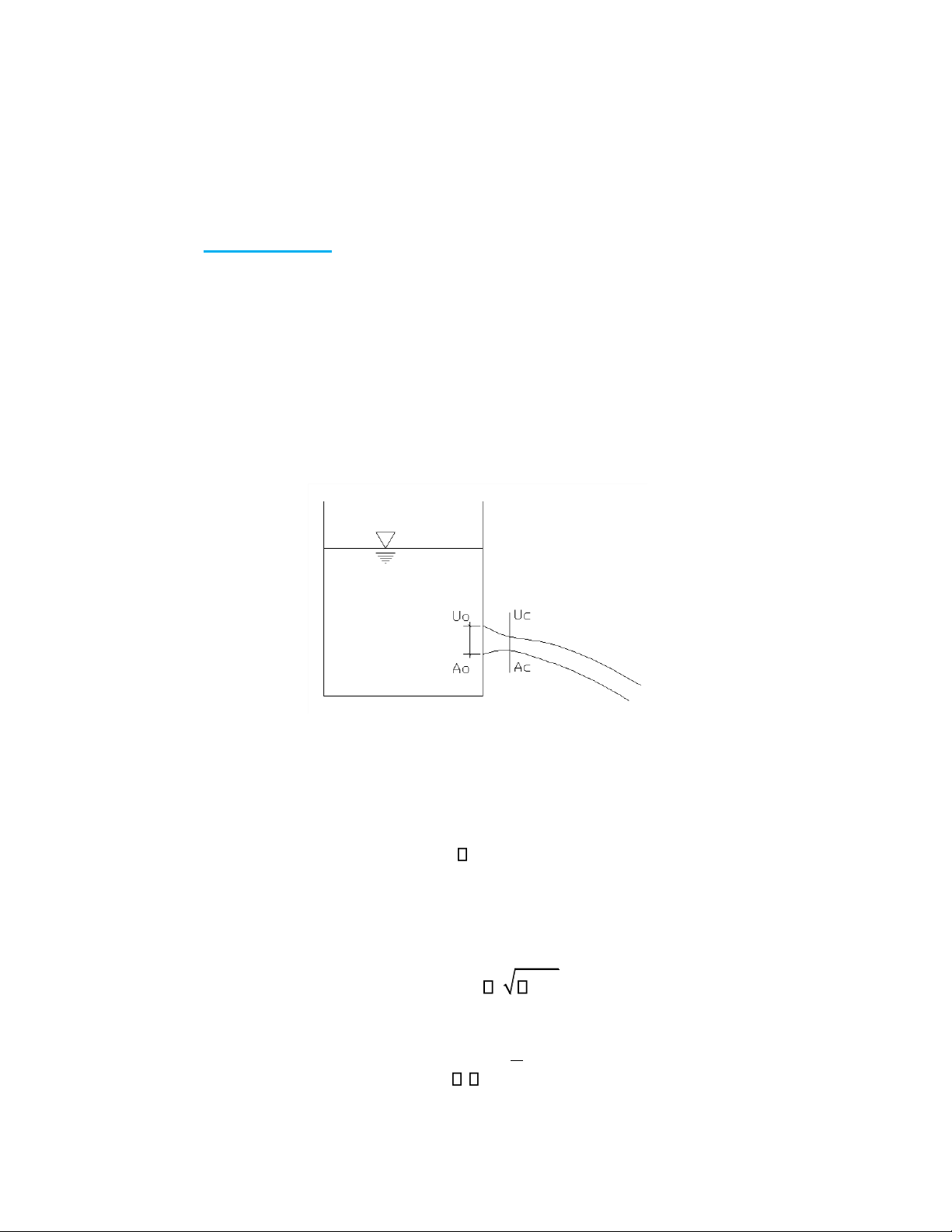
of area. The actual discharge Q is given by: (1) Q u Ac c
and if the jet discharged at the idea velocity uo over the orifice area Ao, the the discharge Qo would be: (2) Q u A A gH o o o o 2 o
So, from the definition of the coefficient of discharge, (3) Q u Ac c Cd lOMoAR cPSD| 58583460 Qo u Ao o
or in terms of quantities measured experimentally, (4) Q C A gH CQ d o 2 o d o  Cd Q Ao 2gHo or (5) Q kH o k where
k C A d o 2g => Cd Ao 2g
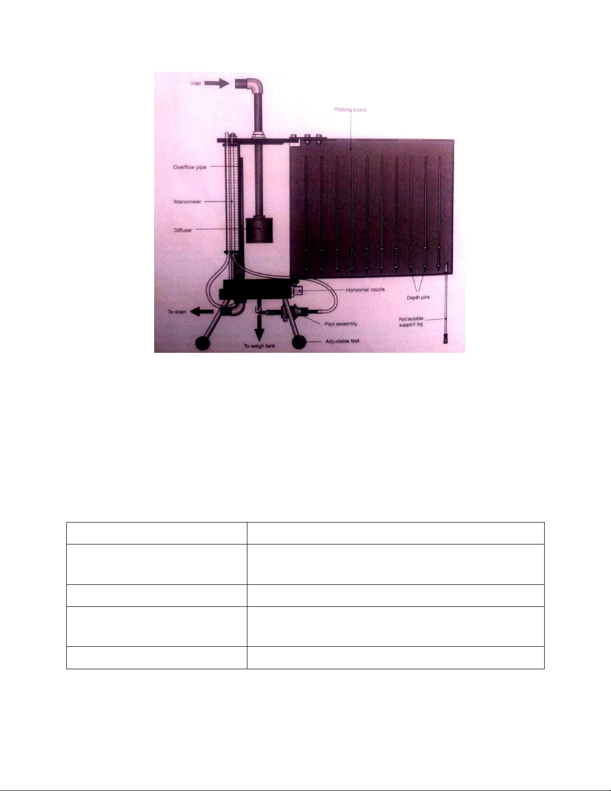
II. Experimental Apparatus
The experimental apparatus consists of the following parts: lOMoAR cPSD| 58583460
Figure 1. General Layout
Table 2. Technical Details Item Details Dimensions and weight
700 mm high x 700 mm long x 400 mm front to (assembled)
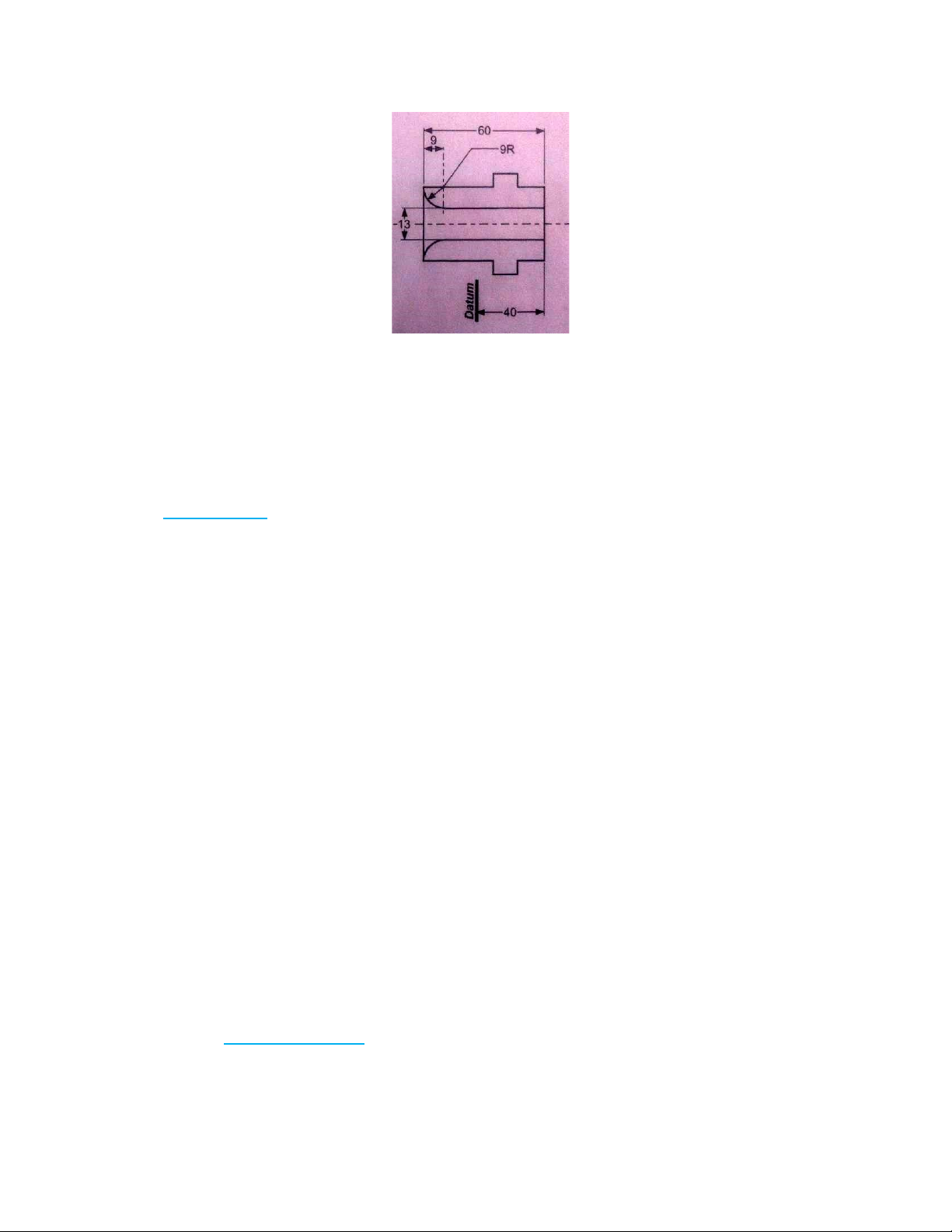
back. 10 kg including nozzles. Manometer scale 100 mm to 390 mm 1 division = 0.1 mm Pitot Micrometer 1 complete turn = 1 mm Set of four Orifice / Nozzles See Figure 2 lOMoAR cPSD| 58583460
Figure 2. Dimensions of the Orifice / Nozzle Dimension in mm
Datum = Distance to internal surface of tank when mounted vertically III. Procedure
(1) Start the pump of the hydraulic bench and adjust the flow so the level in the
tank stays just above the overflow pipe in the tank.
(2) Allow conditions to stabilize and use the hydraulic bench to measure the flow.
Record the Head inside the tank.
(3) Reduce the inlet flow (supply from the hydraulic bench) so that the head falls by about 30 mm.
(4) Allow conditions to stabilize and use the hydraulic bench to measure the flow.
Record the Head inside the tank.
(5) Repeat for decreasing value of head in about 30 mm steps, giving about eight
results over the height of the manometer scale, each time recording head and flow.
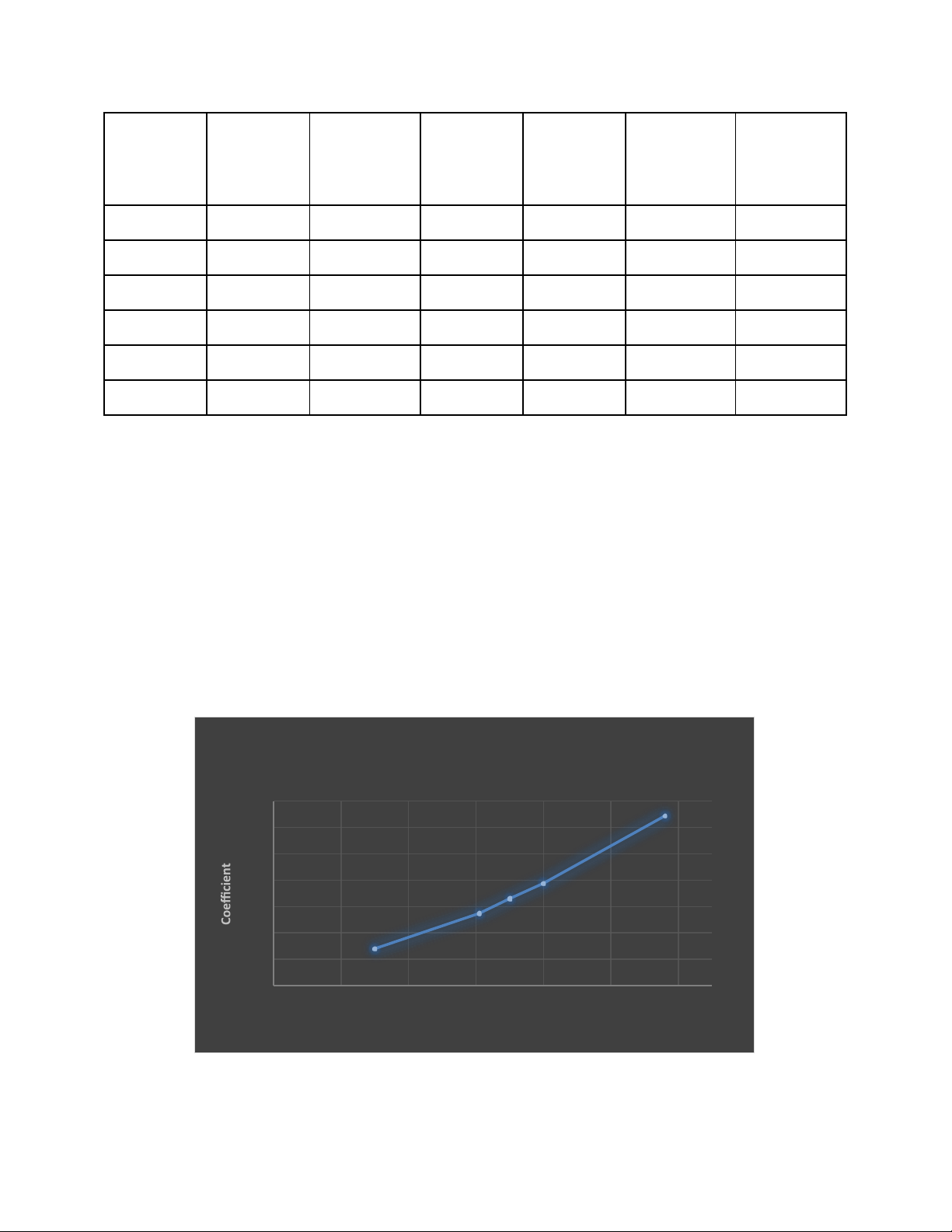
IV. Data Analysis lOMoAR cPSD| 58583460 Water Time Flow (Q) Head H No. Collected 0 Ho ½ (m) Cd (seconds) (m3/s) (m) (kg) 1 6 31.02 1.94x10-4 0.143 0.378 0.872 2 6 30.23 1.98x10-4 0.153 0.391 0.87 3 6 26.54 2.26x10-4 0.176 0.419 0.937 4 6 25.47 2.35x10-4 0.179 0.423 0.965 5 6 24.00 2.50x10-4 0.183 0.428 0.994 6 6 20.96 2.86x10-4 0.188 0.434 1.122
Relationship Between Coefficient of Discharge And Flow 1.15 1.1 1.05 1 0.95 0.9 0.85 0.8
1.70E-04 1.90E-04 2.10E-04 2.30E-04 2.50E-04 2.70E-04 2.90E-04 Flow
Graph 1: Relationship Between Coefficient of Discharge And Flow lOMoAR cPSD| 58583460
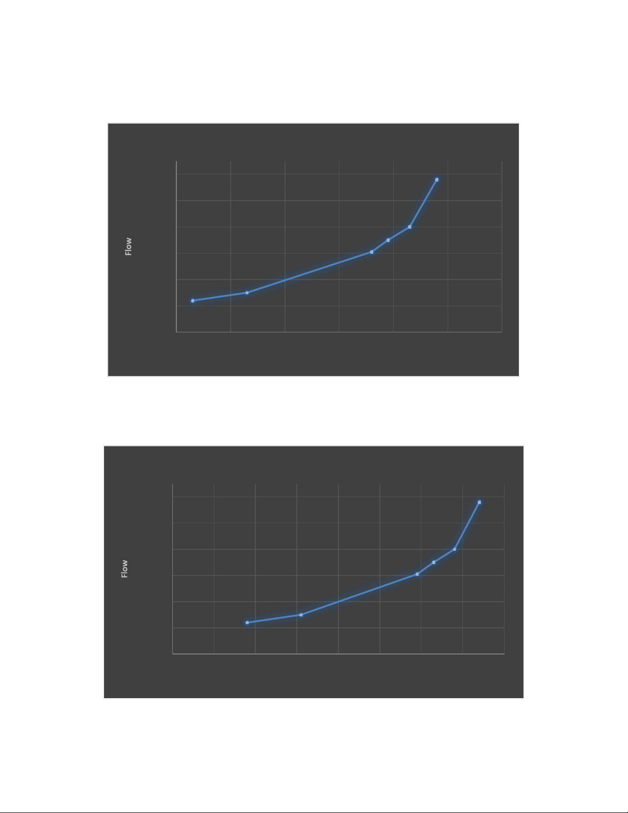
Relationship Between Flow And Head 2.90E-04 2.70E-04 2.50E-04 2.30E-04 2.10E-04 1.90E-04 1.70E-04 0.14 0.15 0.16 0.17 0.18 0.19 0.2 Head
Graph 2: Relationship Between Flow And Head
Relationship Between Flow and Head1/2 2.90E-04 2.70E-04 2.50E-04 2.30E-04 2.10E-04 1.90E-04 1.70E-04 0.36 0.37 0.38 0.39 0.4 0.41 0.42 0.43 0.44 Head1/2
Graph 3: Relationship Between Flow and Head ½ lOMoAR cPSD| 58583460
The slope of the linear results is 1.64x10-3
The average (mean) coefficient of discharge for the orifice is 1.152 V. Conclusion
The experiment succeeds in fulling its objectives:
- to understand the relationship between head and flow for an orifice:
- to show how the coefficient of discharge varies with flow
- to use the head and flow relationship to find the average coefficient of discharge for the orifice.
The error in Cd is determined by the error in measuring Q and H. Furthermore,
Q = 𝑉⁄𝑡 where V is the volume collected in time t, the error of Q is determined by
the error in collecting time t.
Experiment 2: Horizontal Jet Trajectory I. Objective:
The objective of the experiment is to understand the horizontal discharge
characteristics of an orifice or nozzle. II. Theory:
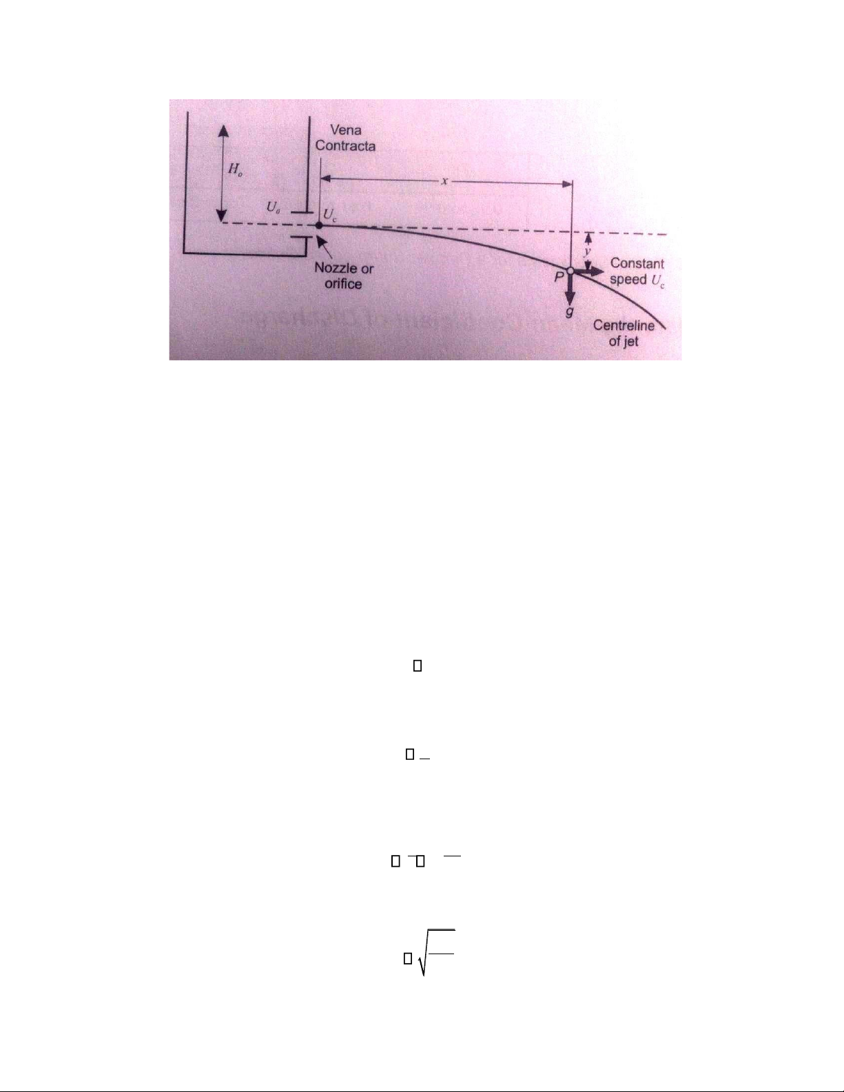
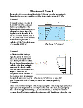
Trajectory from Horizontal lOMoAR cPSD| 58583460
Figure 3. Trajectory from Horizontal
The jet emerges from the nozzle at a velocity uc. At any point P in its trajectory it is
subject to gravitational acceleration (g) in the vertical direction, and has a steady
velocity component in the horizontal direction. As gravity affects its path, the
trajectory should be parabolic. The head (Ho) of water in the tank will affect the
horizontal distance travelled and therefore the curvature of the jet.
Consider a ‘packet’ of water that has travelled a distance x from the vena
contracta to point P in t seconds. It travels at velocity uc in the horizontal direction, (6) x u tc
And over the same time in the vertical direction: (7) 1 y gt2 2
Eliminating t from the two equations gives (8) 1 x2 y g 2 2 uc and (9) gx2 uc lOMoAR cPSD| 58583460 2y u 2 o 2gH o u Cu Cc u o u 2gHo and (10) x2 Cu 4H yo or (11) x 1 C y 4 H u o and (12) x2 y 4Ho
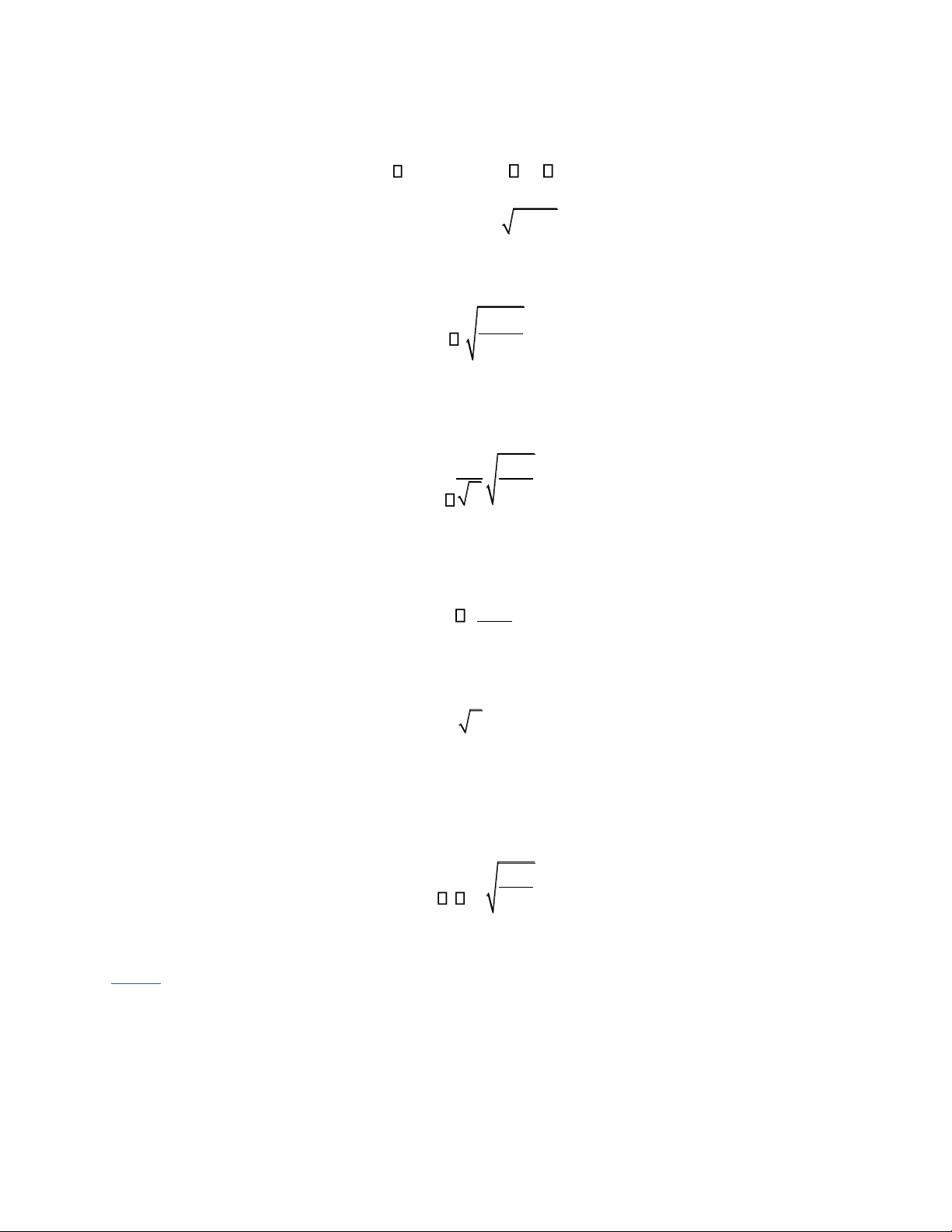
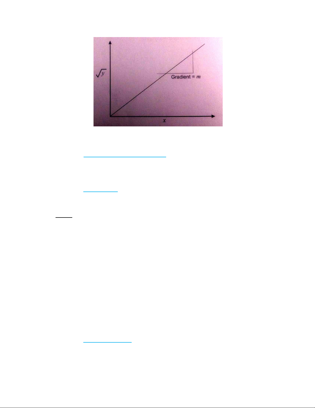
Where the head in the tank (Ho) stays constant, you can find an average value for
the velocity coefficient from a chart of y and x (see Figure 4). The chart should give
linear results. The inverse value of the gradient (m) of this chart substituted back
into Equation 13 should give this average. So: (13) 1 1 Cu 4 H m o
Note: Units of x, y and Ho must be identical (mm or metres) lOMoAR cPSD| 58583460
Figure 4. Chart to help Find Velocity Coefficient
III. Experimental Apparatus
Shown in part 3 of Experiment 1. IV. Procedure
(1) Set the tank for a constant head.
Note: the head of this experiment will be the head of water with respect to
the centre line of the nozzle. The manometer measures with respect to the
bottom of the base plate – roughly 22 mm lower.
(2) Refer to the base plate drawing in Technical Details to allow for this.
(3) Adjust the depth pins so they just touch the surface of the jet without disturbing it.
(4) Mark the positions of the top of the pins onto the chart paper.
(5) Slowly reduce the head in the tank and note how it affects the jet.
(6) Switch off the water supply.
V. Data Analysis Table 1: Report Table lOMoAR cPSD| 58583460
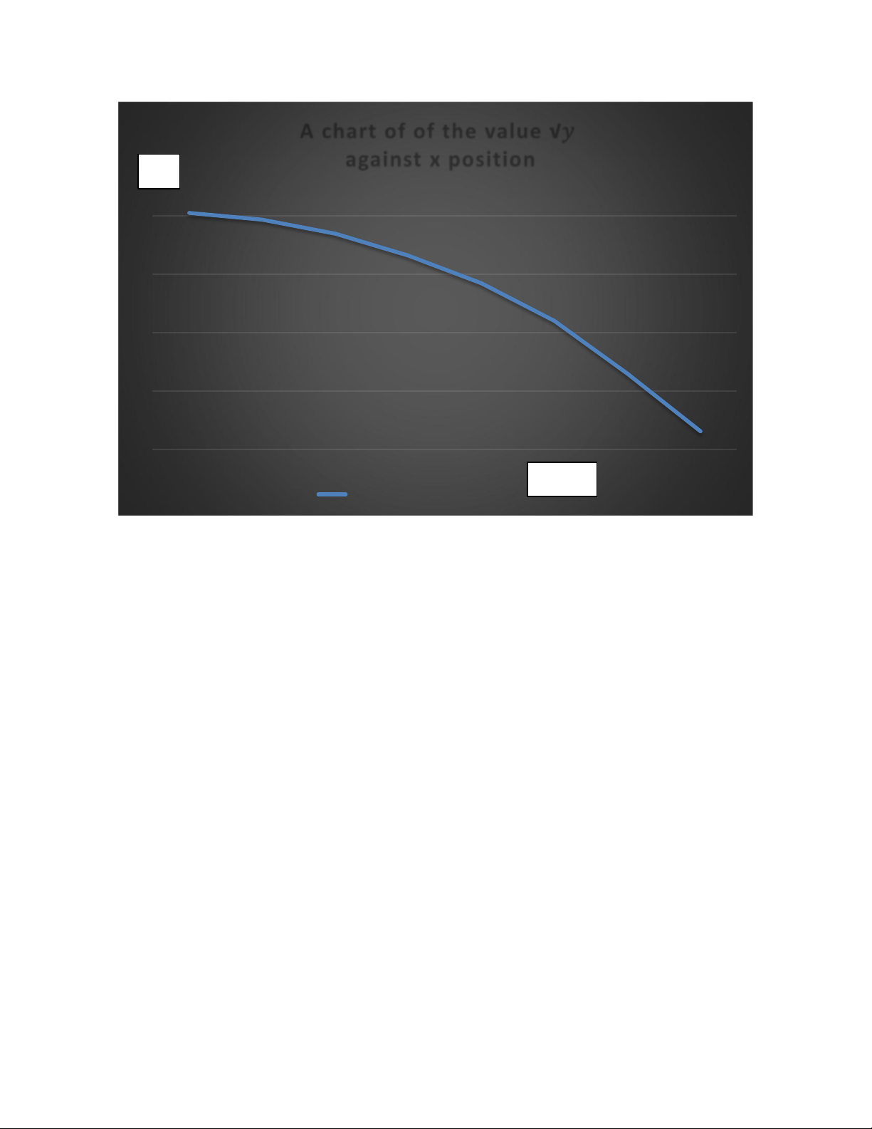
Graph 1 is a chart of y1/2 against x. Using the results of the fifth experiment which Head: 230 (mm) Actual y x (mm) (mm) y1/2 (mm) Predicted y (mm) 0 225 15.0332 0 40 221 14.8660 1.74 80 205 14.3178 6.95 120 181 13.4536 15.65 160 153 12.3693 27.83 200 127 11.2694 43.47 240 95 9.7467 62.60 280 62 7.874 85.21
is near to the predicted result to create the chart. lOMoAR cPSD| 58583460
A chart of of the value √ 𝑦 against x position √ 𝑦 15 13 11 9 7 0 40 80 120 160 200 240 280 x (mm)
A chart of of the value against x position
Graph 1: Chart of y 1 /2 against x
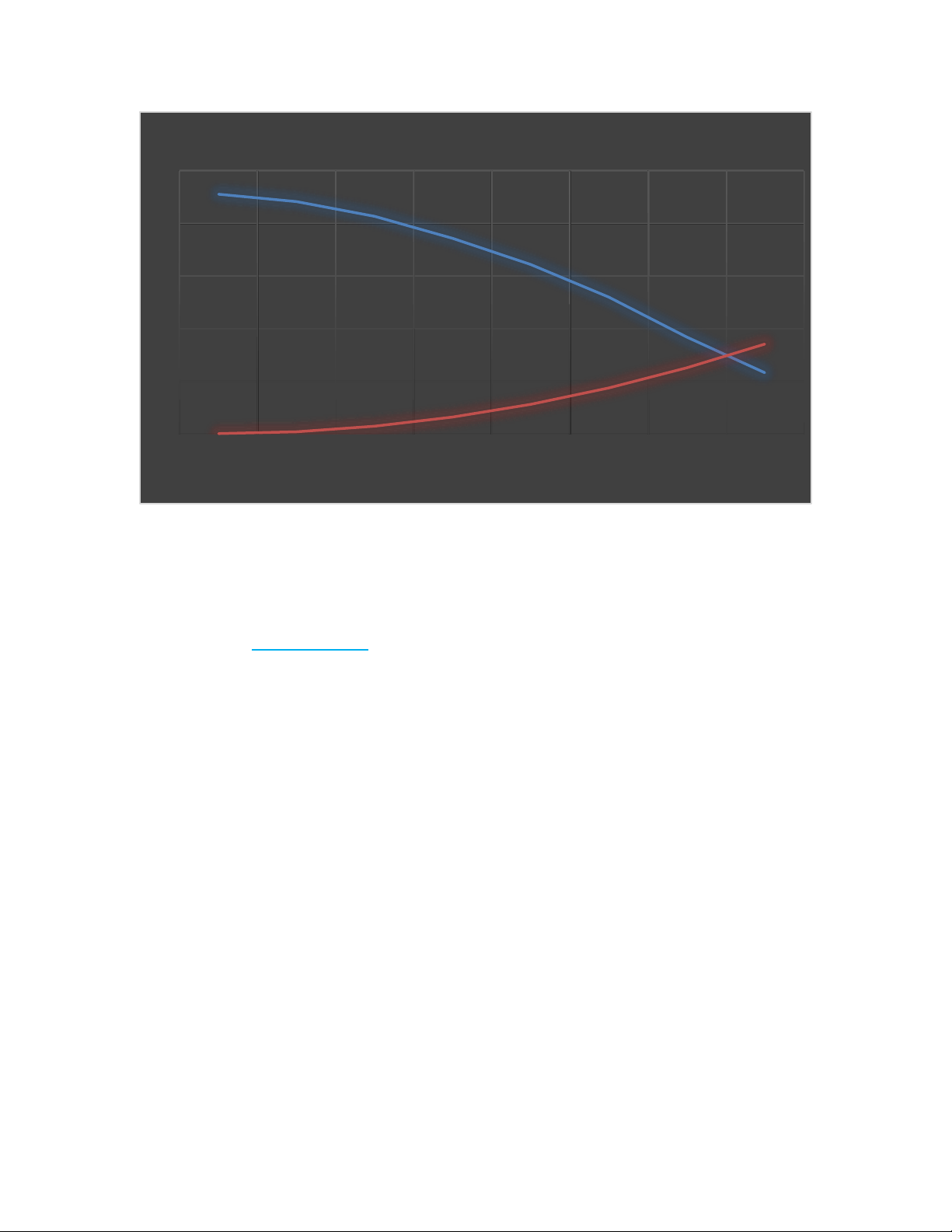
Graph 2 is a chart of the actual flow and the predicted. The predicted flow from
this experiment calculation is quite close to what the flow is actually is. This can be seen in Graph 2 below. lOMoAR cPSD| 58583460 250 225 221 205 200 181 153 150 127 100 95 85.21 62.6 62 50 43.47 0 0 1.74 6.95 15.65 27.83 0 40 80 120 160 200 240 280
Graph 2: Actual Flow and predicted flow VI. Conclusion
The experiment succeeds in fulfilling its objective which is to understand the
horizontal discharge characteristics of an orifice or nozzle. Specifically, the
experiment succeeds in using collected data to produce a predicted flow that is
quite close to the actual flow, which can be seen in Graph 2.
The different between the y predicted and the y actual may occurs because the
error in Ho values or the error when reading the y values from the plotting board.