Lab Report: Fluid Friction Experiments and Analysis | Môn Fluid Mechanics Lab - Trường Đại học Quốc tế, Đại học Quốc gia Thành phố Hồ Chí Minh

lOMoAR cPSD| 58583460
VIETNAM NATIONAL UNIVERSITY – HO CHI MINH CITY
INTERNATIONAL UNIVERSITY SCHOOL OF
Civil Engineering & Management
—------------------------------------------------------------------------
Experiment: FM05: Fluid Friction Apparatus Group Number: 05 No. Name ID 1 Bùi Phú Gia CHCEIU23056 2 Geon Lee CHCEIU23065 3 Nguyễn Huỳnh Gia Huy CHCEIU23016 4 Nguyễn Khánh Tuấn CHCEIU23063 5 CHCEIU23021 Nguyễn Lê Anh Khoa
Academic year: 2023 – 2024
Date of Experiment: 10/04/2024 lOMoAR cPSD| 58583460
VIETNAM NATIONAL UNIVERSITY – HO CHI MINH CITY
INTERNATIONAL UNIVERSITY SCHOOL OF
Civil Engineering & Management
—------------------------------------------------------------------------
----Table of contents----
A. Introduction..............................................................................................2 B.
Preparation...............................................................................................2 C.
Notation...................................................................................................4
Experiment 1: Losses in Straight Pipe
Experiment.....................................................................
I. Objective..................................................................................................5 II.
Theory......................................................................................................5 III.
Experimental Apparatus...........................................................................7 IV.
Procedure ................................................................................................8 V.
Calculation..............................................................................................10 VI.
Conclusion (smooth pipe).......................................................................11
VII.Conclusion (rough pipe)..................................................................................................
Experiment 2: Losses in Bends Experiments.............................................................................
I. Objective................................................................................................13 II.
Theory....................................................................................................13 III.
Experimental Apparatus.........................................................................14 IV.
Procedure ..............................................................................................14 V.
Calculation..............................................................................................15
VI. Conclusion..............................................................................................16
Experiment 3: Sudden Expansion and Sudden Contraction Experiments..................................
I. Objective................................................................................................17 II.
Theory....................................................................................................17 III.
Procedure...............................................................................................18 IV.
Experimental Results..............................................................................19 V.
Analysis..................................................................................................20 VI.
Conclusion..............................................................................................24 A. A. Introduction
Fluid mechanics, a cornerstone of engineering and physics, delves into the behavior and characteristics of
fluids in motion and at rest. One fundamental aspect of fluid mechanics is understanding the intricate
interplay between fluids and solid surfaces, particularly when it comes to the phenomenon of fluid friction. lOMoAR cPSD| 58583460
VIETNAM NATIONAL UNIVERSITY – HO CHI MINH CITY
INTERNATIONAL UNIVERSITY SCHOOL OF
Civil Engineering & Management
—------------------------------------------------------------------------
Fluid friction, also known as viscous drag, refers to the resistance encountered by a fluid as it flows past a
solid surface or through a conduit. This resistance arises due to the internal friction within the fluid itself and
its interactions with the boundary surfaces.
To comprehensively study fluid friction and its implications, engineers and researchers rely on
sophisticated experimental setups known as fluid friction apparatus. These apparatuses are meticulously
designed to provide a controlled environment where various parameters affecting fluid friction can be
measured and analyzed with precision. From determining friction coefficients to investigating flow regimes
and boundary layer characteristics, fluid friction apparatus plays a pivotal role in advancing our understanding of fluid dynamics.
This report aims to explore the intricacies of fluid friction apparatus, elucidating their components,
operation principles, and applications in experimental fluid mechanics. By shedding light on these
apparatuses, we can appreciate their significance in unraveling the complexities of fluid flow and friction, thus
paving the way for innovations in fields ranging from aerospace engineering to renewable energy. B. Preparation
Bleed Air From All Pipes and Instruments
Before taking any readings, bleed out any air trapped in the circuit, tapping points, connecting
tubes, pressure gauges and Piezometer tubes.
To bleed the connection pipes and piezometer •
Obtain the suitable bucket (10 Litre capacity) to avoid water spills. •
Connect and turn on the cold water supply to maximum flow, open the outlet valve on the circuit you
are testing and wait for any trapped air to leave the circuit. •
Close the outlet valve on the circuit you are testing. •
Select suitable lengths of connecting tube and place one end into the bucket. Connect the other ends
to the tapping points you wish to use. •
Wait until all the air has been forced out of the connecting pipes and quickly connect the free ends of
the pipes from out of the bucket to the pair of tappings on the Piezometers you wish to use. •
Open the valve in the cap at the manifold (top of the Piezometer) and allow the piezometer to fill up.
Release the valve when the Piezometer tubes are full of water. •
Reduce the cold water supply to a low rate of flow and open the outlet valve on the circuit you are testing. •
Open the valve cap on the Piezometer manifold again and allow the pressure to equalize in the tubes. lOMoAR cPSD| 58583460
VIETNAM NATIONAL UNIVERSITY – HO CHI MINH CITY
INTERNATIONAL UNIVERSITY SCHOOL OF
Civil Engineering & Management
—------------------------------------------------------------------------
The self sealing tappings at the base of the Piezometer will help to keep the tubes full of water between
experiments, as long as care is taken when you use to connecting tubes.
To alter the relative heights of the water column use the hand pump (supplied) to increase the manifold
pressure, or release the pressure by pressing the centre of the valve in the manifold cap.
To bleed the pressure gauge •
Use the length of pipe (supplied) to connect between the gauge tappings (marked ‘+’ and ‘-’ ) and the
tappings at the valve you wish to monitor. •
Open the valve fully, increase the water supply to maximum flow and temporarily block the outlet pipe
(hold your hand over the end of the pipe) to give maximum pressure in the circuit and at the valve. •
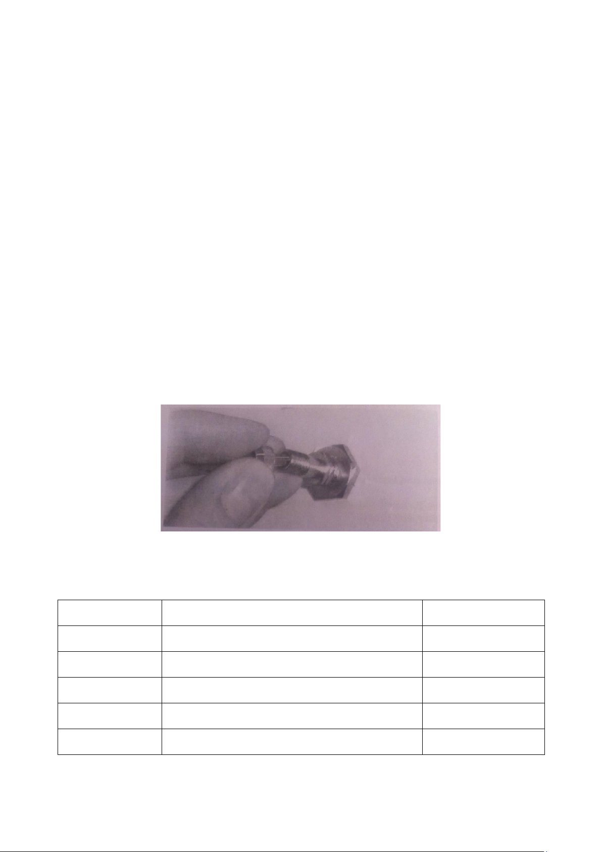
Unscrew the cap from each bleed valve (above the pressure gauge). Turn each of the caps around and
press them into each bleed valve body, this opens the valves (see Figure 11). •
Keep the valve open until all the air has passed out of pipe. •
Remove the block on the outlet and adjust the flow to that needed for the experiment.
Figure 1. Turn the Bleed Valve Caps around and Press them into the Valve Body C. Notation
The following symbols are used in the theory and calculations for the experiments: Symbol Description Units Q Volumetric Flow Rate m3/s h Head m u Flow Velocity m/s d Pipe Diameter m v Kinematic Viscosity m2/s lOMoAR cPSD| 58583460
VIETNAM NATIONAL UNIVERSITY – HO CHI MINH CITY
INTERNATIONAL UNIVERSITY SCHOOL OF
Civil Engineering & Management
—------------------------------------------------------------------------ l
Length of pipe (between tappings) m f Fiction Factor - g Acceleration due to Gravity m/s2 k Loss Factor - ks Diameter of Sand Grains m A Cross Sectional Area of Pipe m2 Re Reynolds Number - lOMoAR cPSD| 58583460
VIETNAM NATIONAL UNIVERSITY – HO CHI MINH CITY
INTERNATIONAL UNIVERSITY SCHOOL OF
Civil Engineering & Management
—------------------------------------------------------------------------
Experiment 1: Losses in Straight Pipes Experiments I. Objective:
The objective of the exercise is to do determine the losses in smooth and roughened pipes. II. Theory
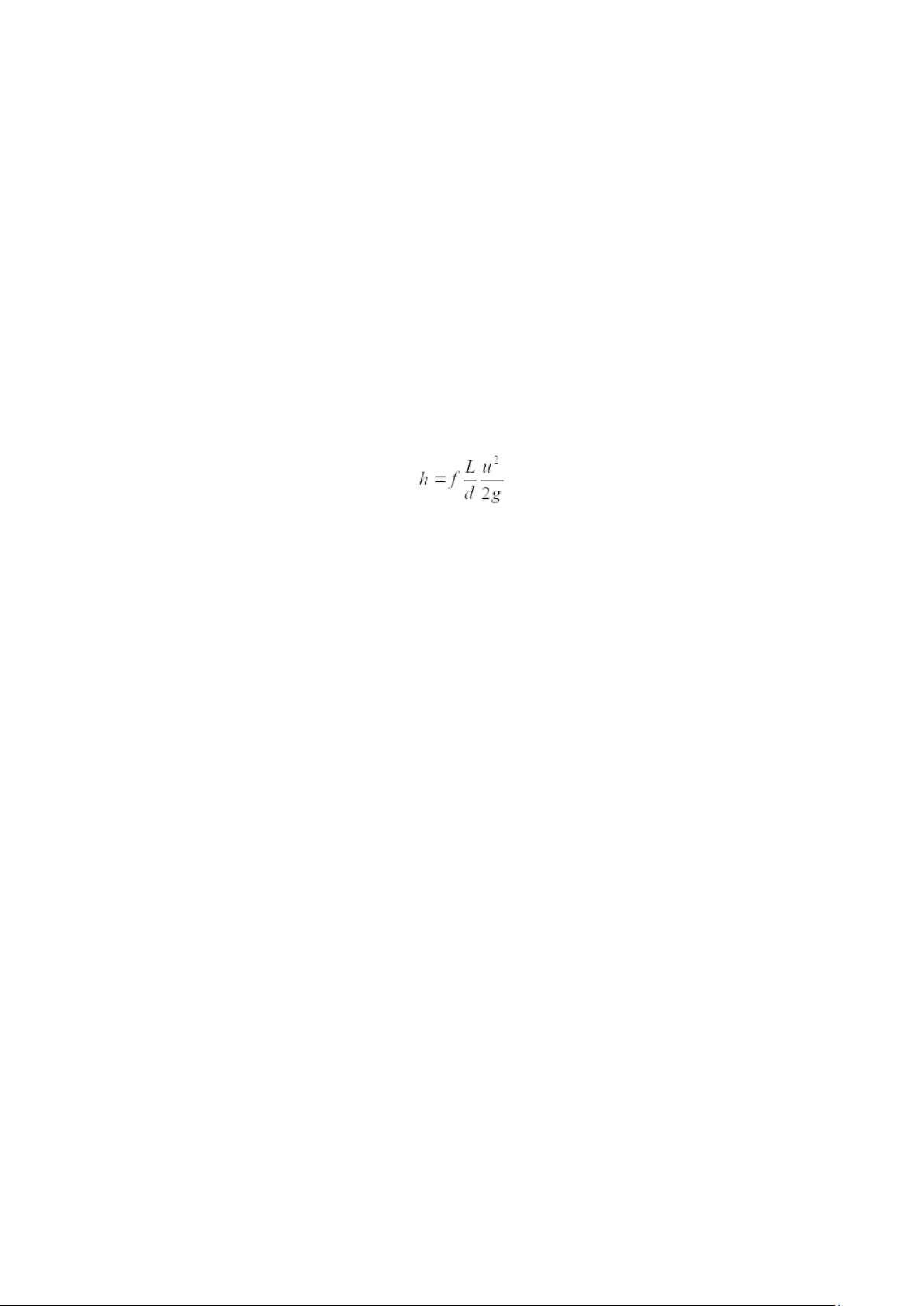
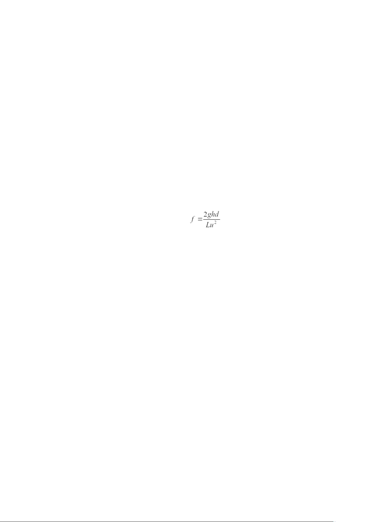
As fluid flow through a straight pipe, energy is dissipated due to turbulence and friction. This energy can be
measured by the head loss for a length of pipe. Much research has been done into the losses in pipes, and it
has been show that the head loss, h, can be represented by a friction factor f, where (1) lOMoAR cPSD| 58583460
VIETNAM NATIONAL UNIVERSITY – HO CHI MINH CITY
INTERNATIONAL UNIVERSITY SCHOOL OF
Civil Engineering & Management
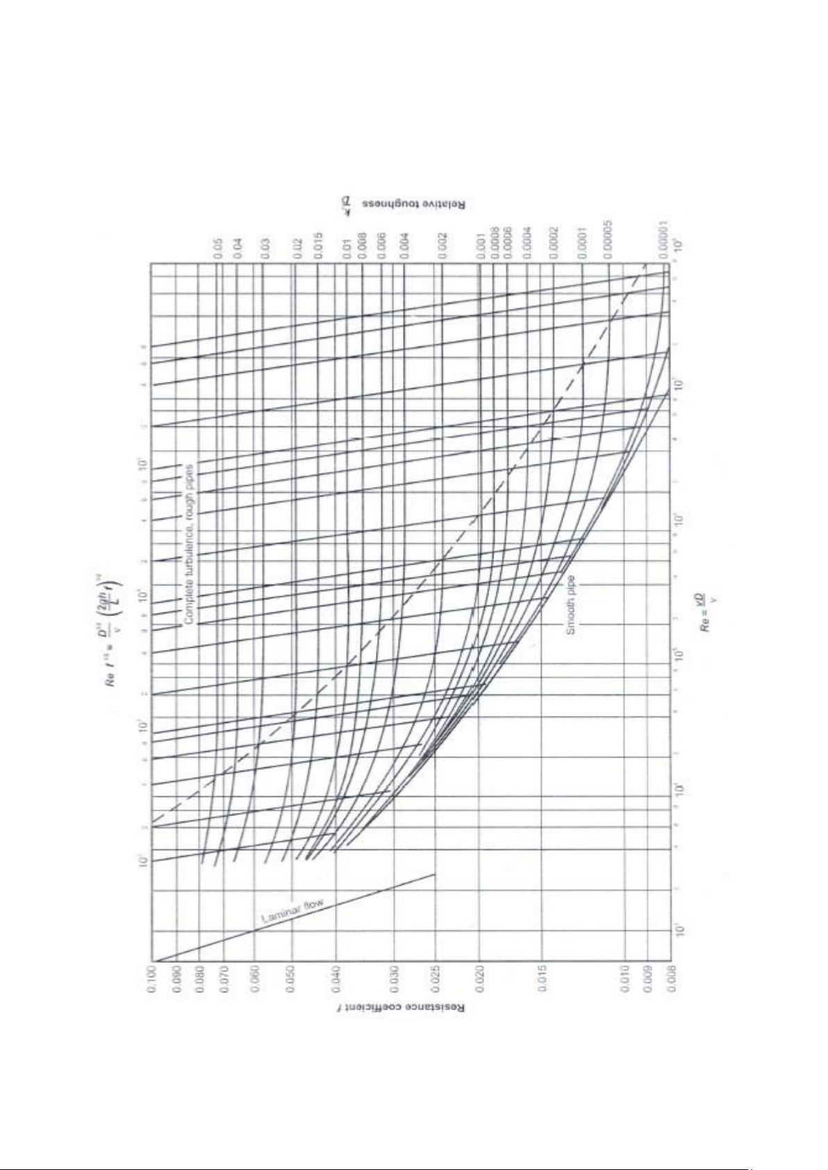
—------------------------------------------------------------------------ Figure 2. Moody Chart lOMoAR cPSD| 58583460
VIETNAM NATIONAL UNIVERSITY – HO CHI MINH CITY
INTERNATIONAL UNIVERSITY SCHOOL OF
Civil Engineering & Management
—------------------------------------------------------------------------
III.Experimental Apparatus lOMoAR cPSD| 58583460
VIETNAM NATIONAL UNIVERSITY – HO CHI MINH CITY
INTERNATIONAL UNIVERSITY SCHOOL OF
Civil Engineering & Management
—------------------------------------------------------------------------
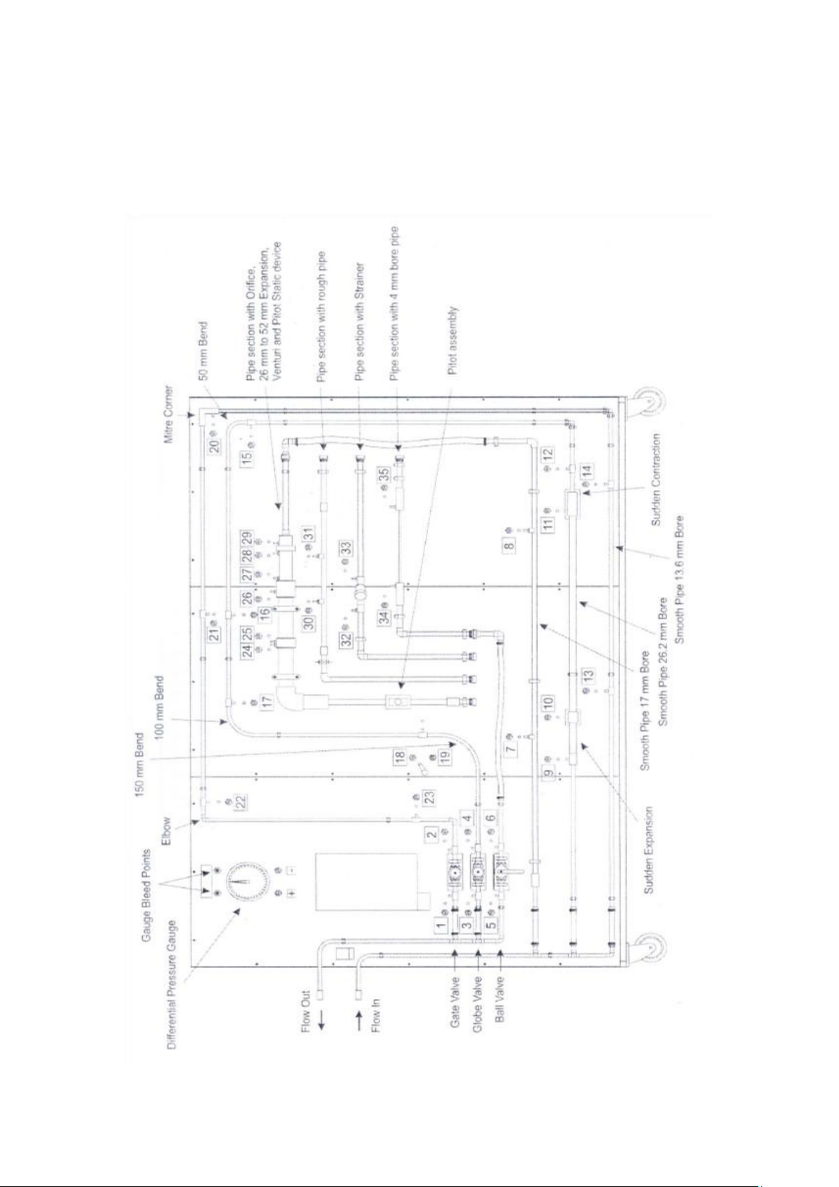
Figure 3. Layout of the equipment
Table 1. Pipes Fittings and Their Tappings Distances Tapping Item Details Between Numbers Tappings Gate Valve - 1, 2 - Globe Valve - 3, 4 - Ball Valve - 5, 6 - Smooth Pipe 17 mm Diameter Bore 7, 8 912 mm Sudden Enlargement 13.6 mm to 26.2 mm 9, 10 - Sudden Contraction 26.2 mm to 13.6 mm 11, 12 - Smooth Pipe 26.2 mm Diameter Bore 10, 11 912 mm Smooth Pipe 13.6 mm Diameter Bore 13, 14 912 mm Radius Bend 50 mm 15, 16 920 mm 13.6 mm Diameter Radius Bend 100 mm 17, 18 864 mm 13.6 mm Diameter Radius Bend 150 mm 19, 4 652 mm 13.6 mm Diameter Mitre Corner - 20, 21 - Elbow 13.6 mm Radius 22, 23 - Orifice 20 mm Diameter 24, 25 - Expansion 26 mm to 52 mm 26, 27 - Venturi d1 = 26 mm Diameter 28, 29 - d2 = 16 mm Diameter Rough Pipe 17 mm Diameter Bore 30, 31 200 mm 14 mm Effective Diameter Strainer
Includes Two Different Filters 32, 33 - Smooth Pipe 4 mm Diameter Bore 34, 35 350 mm Inlet Pipe Coloured White - - Outlet Pipe Coloured Black - - IV.Procedure
1) Prepare Collected Data Tables. lOMoAR cPSD| 58583460
VIETNAM NATIONAL UNIVERSITY – HO CHI MINH CITY
INTERNATIONAL UNIVERSITY SCHOOL OF
Civil Engineering & Management
—------------------------------------------------------------------------
2) Close the Globe valve and the Ball valve (light blue and grey circuits). Open the Gate valve (dark blue circuit) half of a turn.
3) Turn on the cold water supply and wait for any trapped air to leave the circuit, then close the Gate valve.
4) Connect one set of Piezometer tubes to tapping 13 (upstream) and tapping 14 (downstream) for
example. If necessary, bleed the pipes as describes in ‘Set up’.
5) Use the hand pump if necessary to adjust the pressure in Piezometer tubes until the level is halfway
up the scale. The level in each of the Piezometer should the same, if not then check for air bubbles or leaks.
6) Fully open the gate valve and wait for the flow to settle. Record the readings on the Piezometer into your Collected Data Tables.
7) Use the Gate valve to reduce the flow rate in five suitable steps to give a good spread of results.
8) Repeat for the rough pipe (tapping 30 – tapping 31).Close Globe valve and Gate valve, open the Ball valve (grey circuit).
Table 2. Collected Data Table for Smooth Pipe
Internal Diameter (d) = 13,6 mm Area (A) = 145,27 mm2 Length (l) = 912 mm Pipe Type = Smooth pipe Piezometer Reading Water Quantity No. Time (seconds) Upstream Tapping Downstream Tapping (m3 or liters) 13 (mm) 14 (mm) 1 0,012 19,43 640 618 2 0,012 16,57 729 670 3 0,012 11,68 747 680 4 0,012 9,84 752 680 5 0,012 15,88 751 684 6
Table 3. Collected Data Table for Rough Pipe Internal Diameter (d) = 17 mm Area (A) = 226,98 mm2 Length (l) = 200 mm Pipe Type = Rough Pipe Piezometer Reading Water Quantity No. Time (seconds) Upstream Tapping Downstream Tapping (m3) 30 (mm) 31 (mm) lOMoAR cPSD| 58583460
VIETNAM NATIONAL UNIVERSITY – HO CHI MINH CITY
INTERNATIONAL UNIVERSITY SCHOOL OF
Civil Engineering & Management
—------------------------------------------------------------------------ 1 0,012 19,43 200 200 2 0,012 16,57 264 255 3 0,012 11,68 275 280 4 0,012 9,84 285 255 5 0,012 15,88 282 288 6 lOMoAR cPSD| 58583460
VIETNAM NATIONAL UNIVERSITY – HO CHI MINH CITY
INTERNATIONAL UNIVERSITY SCHOOL OF
Civil Engineering & Management
—------------------------------------------------------------------------ V. Calculation a. Smooth Pipes
(a) For each pipe, calculate the flow rate (Q) and hence the flow velocity (u) u = Q / A (2)
To follow a meaningful comparison to be made between pipes of different diameter and different flow
rates, the Reynolds number, Re, for each test point is calculated, where Re = ud / v (3)
Given that v = 1.004 x 10-6 for water at 20oC
(b) Calculate the friction factor, f, and the Reynolds number, Re, for each of the smooth pipes at each flow
rate. The friction factor is measured from Equation1
Calculate the Blasius friction factor for each test point and compare to the measured value of f. For a
smooth pipe, the friction factor is given by the empirical Blasius formula. f = 4*0.079(Re)-1/4 (4)
The smooth pipes used on the apparatus are good quality with a generally smooth internal surface.
(c) Do these value suggest that the pipe are perfectly smooth? From these calculations, what effect does
the pipe diameter have on the apparent smoothness? b. Roughened Pipes
Figure 2 shows graph produced by the American engineer Lewis Moody (1880-1953) which show the
relationship between friction factor and Reynolds number for different level of pipe roughness. The line for
a smooth pipe is the same as the Blasius formula.
(a) From the recorded results, calculate the f factor from the Equation1 and the Reynolds number for the roughened pipe.
(b) Compare the f factor for the roughened pipe with the value from the Moody graph.
(c) This pipe is coated internally with sand that has an average grain size of 0.5 mm (see Figure 2). The
effective pipe diameter is 14 mm, so ks/d = 0.036
Table 4a. Report Table for smooth pipe lOMoAR cPSD| 58583460
VIETNAM NATIONAL UNIVERSITY – HO CHI MINH CITY
INTERNATIONAL UNIVERSITY SCHOOL OF
Civil Engineering & Management
—------------------------------------------------------------------------
Interna l Diameter (d) = 13,6 mm Area (A) = 145,27 mm2 Length (l) = 912 mm Pipe Type = Smooth pipe Piezometer Reading Water Upstream Downstream Flow Time Flow Rate Blasius No. Quantity Tapping 13 Tapping 14 Velocity Re f (seconds) (Q) (m3/s) f (m3) (mm) (mm) Difference (m/s) ( ) (m) 1 0,012 19,43 6,18 x 10-4 640 618 0,022 4,25 57568 3,56 x 10-4 1,007 2 0,012 16,57 7,24 x 10-4 729 670 0,059 4,98 67458 6,96 x 10-4 1,007 3 0,012 11,68 1,03 x 10-4 747 680 0,067 0,7 9482 0,04 1,011 4 0,012 9,84 1.22 x 10-3 752 680 0,072 8,4 113784 2,99 x 10-4 1,006 5 0,012 15,88 7,56 x 10-4 751 684 0,067 5,20 70438 7,25 x 10-4 1,007 VI.Conclusion (smooth pipe)
The data presented in the table provides a comprehensive insight into the experimental investigation
of flow characteristics through a smooth pipe with specific dimensions. Through systematic measurement
and analysis, key parameters such as flow rate, flow velocity, Reynolds number (Re), and friction factor (f)
have been determined, offering valuable insights into the behavior of fluid flow within the given system.
Observations from the experimental trials reveal notable trends in flow rate and velocity, as well as
corresponding pressure differentials measured using piezometers. These findings underscore the importance
of understanding flow dynamics within smooth pipes and highlight the role of pipe geometry and surface
characteristics in determining flow behavior.
Comparisons with theoretical predictions, such as those derived from Blasius' equation for friction
factor estimation, demonstrate the consistency between experimental data and established models, thus
validating the experimental methodology employed.
Overall, the data presented in the table serves as a foundational resource for further exploration and
analysis of fluid flow in smooth pipes. By elucidating the intricacies of flow behavior and frictional losses, this
research contributes to the development of more accurate predictive models and informs the design and
optimization of piping systems across various engineering applications. Continued experimentation and
analysis hold the potential to unveil deeper insights into fluid dynamics and pave the way for advancements
in engineering practice and theory. lOMoAR cPSD| 58583460
VIETNAM NATIONAL UNIVERSITY – HO CHI MINH CITY
INTERNATIONAL UNIVERSITY SCHOOL OF
Civil Engineering & Management
—------------------------------------------------------------------------ Internal Diameter (d) = 17 mm Area (A) = 226, 98 mm2 Length (l) = 200 mm
Pipe Type (Smooth/Rough) = rough pipe Piezometer Reading Water Upstrea Flow Time Flow Rate No. Quantity m Downstream Velocity Re f Bl (seconds) (Q) (m3/s) (m3 or L) Tapping Tapping 31 Difference (m/s) 30 (mm) (mm) ( ) (m) 1 0,012 19,43 6,18x 10-4 200 200 0 2,72 46056 0 1, 2 0,012 16,57 7,24x 10-4 264 255 0.009 3,2 54183 1,47 x 10-3 1, 3 0,012 11,68 1,03x 10-3 275 280 0,005 4,54 76873 4,04 x 10-4 1, 4 0,012 9,84 1,22x 10-3 285 255 0,03 5,37 90926 1,73 x 10-3 1, 5 0,012 15,88 7,56x 10-4 282 288 0,006 3,33 56384 9,02 x 10-4 1,
Table 4b. Report Table for rough pipe 00 00 00 00 00 VII.Conclusion (rough pipe)
The data presented in the rough pipe table elucidates the experimental investigation of flow
characteristics through a rough pipe with specific dimensions. Through meticulous measurement and
analysis, key parameters such as flow rate, flow velocity, Reynolds number (Re), and friction factor (f) have
been determined, shedding light on the behavior of fluid flow in the given system.
The observed trends in flow rate and velocity, in conjunction with the corresponding pressure
differentials measured using piezometers, provide valuable insights into the effect of roughness on flow
resistance within the pipe. Moreover, the calculated Reynolds numbers and friction factors offer a
quantitative understanding of the flow regime and frictional losses experienced by the fluid. lOMoAR cPSD| 58583460
VIETNAM NATIONAL UNIVERSITY – HO CHI MINH CITY
INTERNATIONAL UNIVERSITY SCHOOL OF
Civil Engineering & Management
—------------------------------------------------------------------------
Comparisons with theoretical models, such as Blasius' equation for friction factor estimation, reveal
the extent to which experimental findings align with established theories, thus validating the experimental
approach and results obtained.
Overall, the data presented in the table serves as a foundation for further analysis and exploration
of fluid flow in rough pipes, facilitating the optimization and design of piping systems across various
engineering applications. Further experimentation and analysis may yield deeper insights into the intricacies
of fluid dynamics and aid in the development of more accurate predictive models for practical engineering scenarios.
Experiment 2: Losses in Bends Experiments I. Objective:
The objective of the experiment is to determine the head loss in bends. II. Theory:
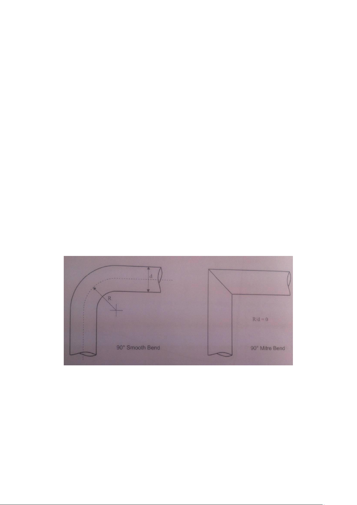
When a fluid flows round a bend, energy losses occur due to flow separation, wall friction and some secondary
– flow patterns caused by the bend. Bends maybe characterized by the ratio of bend radius to internal
diameter, R/d, where gently sweeping bends may have values of 10 or more, or an abrupt ‘miter’ bend would be 0.
Figure 4. Bend Radius and Pipe Diameter Relationship
For tight bends such as mitres, the losses will be mainly due to flow separate and secondary flow patterns.
For more gentle bends, flow separation and wall friction will predominate.
These losses can be represented with a loss factor, k. hB = kB u2 / 2g (5) lOMoAR cPSD| 58583460
VIETNAM NATIONAL UNIVERSITY – HO CHI MINH CITY
INTERNATIONAL UNIVERSITY SCHOOL OF
Civil Engineering & Management
—------------------------------------------------------------------------
However, it is helpful to differentiate between the total loss round the bend (kL, hL), and the loss due to the
bend geometry, (kB, hB) which ignores wall friction losses. The losses around the bend are created by the
bend losses and an additional loss due to the length of pipe that it is made from. This additional loss must
be added to hB to find kL and hL. The loss due to bend geometry is found by measuring the head loss
between the tappings and deducting the calculated head loss for an equivalent length of straight pipe.
In order to give good, steady manometer readings, the pressure tappings after the bends on this equipment
are positioned downstream of the bends. The distance between tappings for each bend are given in Table 1.
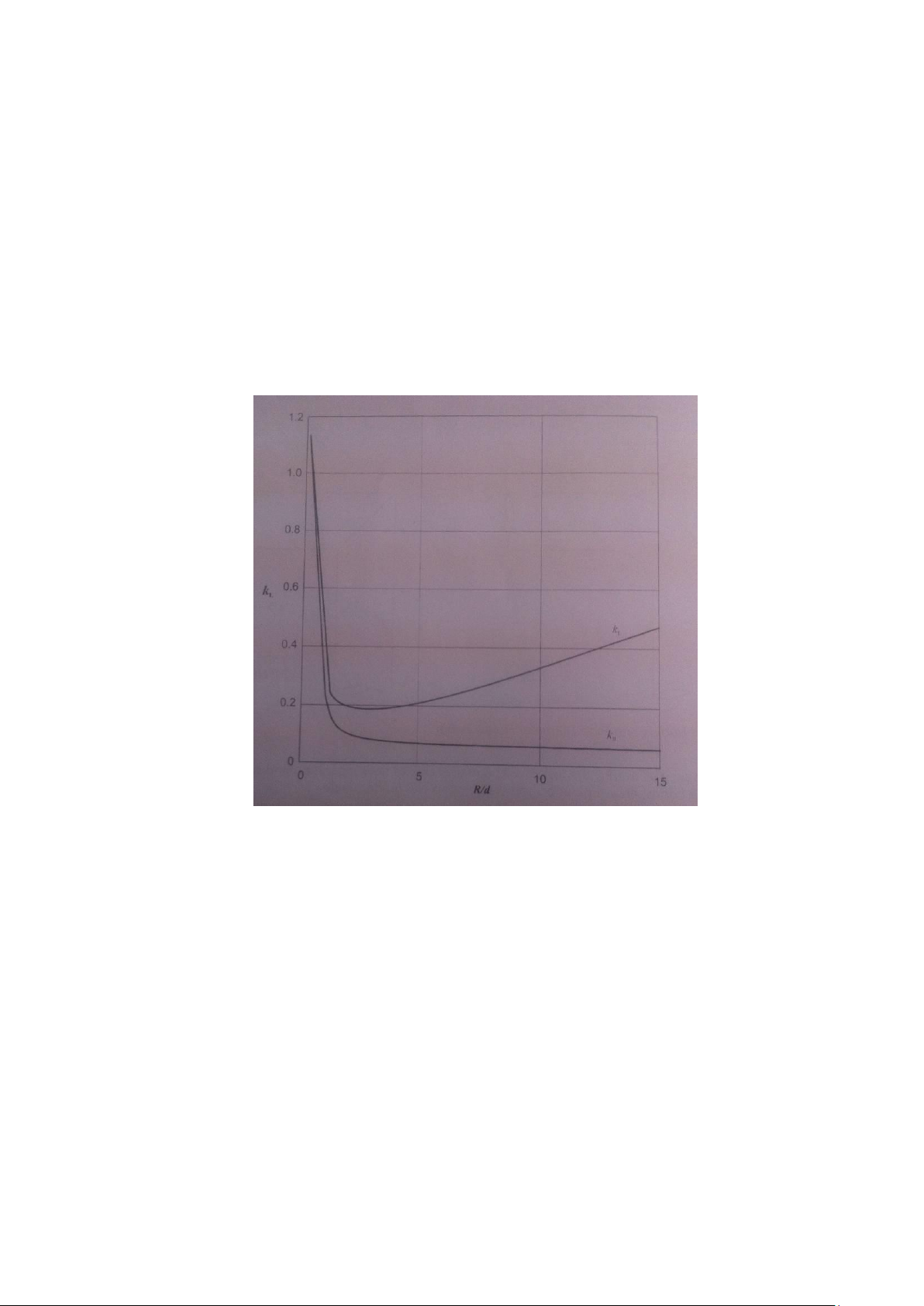
Figure 5. Loss Coefficients for Smooth Bends III. Experimental Apparatus
Shown in Part 3 of Experiment 1. IV. Procedure
1) Prepare a Collected Data Table.
2) Close the Globe valve and the Ball valve (light blue and grey circuits). Open the Gate valve (dark blue circuit) half of a turn.
3) Turn on the cold water supply and wait for any trapped air to leave the circuit, then close the Gate valve. lOMoAR cPSD| 58583460
VIETNAM NATIONAL UNIVERSITY – HO CHI MINH CITY
INTERNATIONAL UNIVERSITY SCHOOL OF
Civil Engineering & Management
—------------------------------------------------------------------------
4) Connect one set of three set of Piezometer tubes to Tappings at each side of the bends. If
necessary, bleed the pipes as describes in ‘Set up’.
5) Use the hand pump if necessary to adjust the pressure in Piezometer tubes until the level is halfway
up the scale. The level in each of the Piezometer should the same, if not then check for air bubbles
or leaks. Note that Tappings 18 and 19 are actually the same point, but are selected with the two
way valve next to them. The valve handle points to the tapping that is connected. The valve is fitted
to remove any possibility of pressure imbalance when tappings 4, 19, 18 and 17 are used at the same time.
6) Fully open the Globe gate valve and wait for the flow to settle. Record the Peizometer readings into your tables .
7) Use the Gate valve to reduce the flow rate in five suitable steps to give a good spread of results.
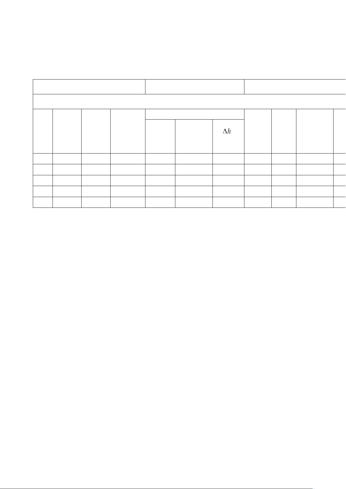
Table 5. Collected Data Table for Bends
Internal Diameter (d) = 13,6 mm Pipe Length (l) = 864 mm Bend Radius (R) = 100 mm Piezometer Reading Water Quantity No. Time (seconds) Upstream Tapping Downstream Tapping (m3) 17 (mm) 18 (mm) 1 0.012 19,43 366 65 2 0.012 16,57 514 50 3 0.012 11,68 534 53 4 0.012 9,84 550 49 5 0.012 15,88 484 54 6 V. Calculation
1) For each test point, calculate the flow velocity, and hence the Reynolds number, following the Equations (2) and (3).
2) Use Blasius equation to find the friction factor f. For a more accurate measure of the frictional head
loss, use the k/d value (0.036) from Experiment 1 to find the f factor from the Moody chart, at the
given Reynolds number. Indicate which one you will use in your computations.
3) Calculate the frictional head loss for an equivalent length of smooth straight pipe hL = fLu2 / 2gd
4) The head loss due to the bend geometry can now be found lOMoAR cPSD| 58583460
VIETNAM NATIONAL UNIVERSITY – HO CHI MINH CITY
INTERNATIONAL UNIVERSITY SCHOOL OF
Civil Engineering & Management
—------------------------------------------------------------------------
5) Standard graphs of kL against R/d show that kL has minimum value at R/d of between 2 and 3 (see
Figure 5). Why do you think this is? lOMoAR cPSD| 58583460
VIETNAM NATIONAL UNIVERSITY – HO CHI MINH CITY
INTERNATIONAL UNIVERSITY SCHOOL OF
Civil Engineering & Management
—-----------------------------------------------------------------------Table
6. Report Table for Bends
Internal Diameter (d) = 13,6 mm Pipe Length (l) = 864 mm Bend Radius (R) = 100 mm Piezometer Reading kL Water Flow Straight Time
Flow Rate Upstream Downstream Bend No. Quantity Difference Velocity Re f Pipe u2/2g
(seconds) (Q) (m3/s) Tapping Tapping 18 Loss (m3 or L) ( ) (m) (m/s) Loss 17 (mm) (mm) 1 0.012 19,43 6,18x 10-4 366 65 301 4.26 57705 0.02 1.18 299.82 0.92 0.3 2 0.012 16,57 7,24x 10-4 514 50 464 4.99 67594 0.02 1.61 462.39 1.27 0.3 3 0.012 11,68 1,03x 10-3 534 53 481 7.10 96175 0.02 3.26 477.74 2.57 0.3 4 0.012 9,84 1,22x 10-3 550 49 501 8.41 113920 0.02 4.58 496.42 3.60 0.3 5 0.012 15,88 7,56x 10-4 484 54 430 5.21 70574 0.02 1.76 428.24 1.38 0.3 VI. Conclusion
Based on the data presented in Table 6 for bends, it is evident that variations in water quantity, time, flow rate, piezometer readings, flow velocity,
and losses are observed across different instances. These variations are influenced by factors such as the internal diameter, pipe length, and bend radius. As
the flow passes through the bends, changes in flow velocity and losses occur, contributing to fluctuations in the measured parameters. The analysis of these
findings provides valuable insights into the hydraulic behavior of bends within the system. Further investigation and analysis could yield deeper
understanding and potentially inform optimization strategies for hydraulic systems. Pages - 16