Laboratory Exercise 2: Discrete-Time Systems: Time-Domain Representation | Trường đại học sư phạm kĩ thuật TP. Hồ Chí Minh

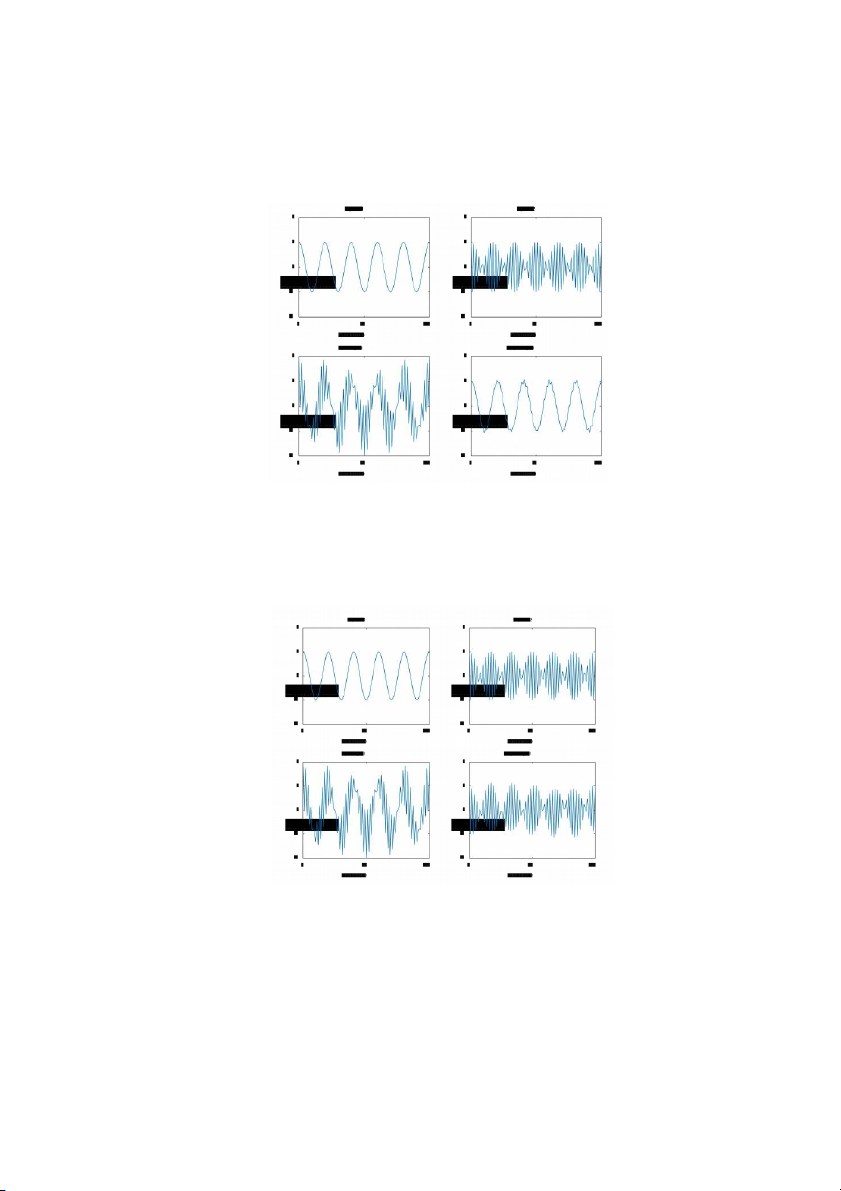
Q2.1: The output sequence generated by running the above program for M = 2 with x[n] = s1[n]+s2[n] as the input is shown below. The component of the input x[n] suppressed by the discrete-time system simulated by this program is - Signal #2, it is a high frequency signal and be suppressed by a low pass filter system; Tài liệu giúp bạn tham khảo, ôn tập và đạt kết quả cao. Mời bạn đọc đón xem!

Thông tin:
35 trang 3 tháng trước

Bình luận

Vui lòng đăng nhập hoặc đăng ký để gửi bình luận.

Laboratory Exercise 2: Discrete-Time Systems: Time-Domain Representation | Trường đại học sư phạm kĩ thuật TP. Hồ Chí Minh

Q2.1: The output sequence generated by running the above program for M = 2 with x[n] = s1[n]+s2[n] as the input is shown below. The component of the input x[n] suppressed by the discrete-time system simulated by this program is - Signal #2, it is a high frequency signal and be suppressed by a low pass filter system; Tài liệu giúp bạn tham khảo, ôn tập và đạt kết quả cao. Mời bạn đọc đón xem!

61 31 lượt tải Tải xuống
Name: Phm Th H ng Giang 18161068 ươ
Lê Anh Đ c 18161062
Section: Group 2
Laboratory Exercise 2
DISCRETE-TIME SYSTEMS: TIME-DOMAIN REPRESENTATION
2.1 SIMULATION OF DISCRETE-TIME SYSTEMS
Project 2.1 The Moving Average System
% Program P2_1
% Simulation of an M-point Moving Average Filter
% Generate the input signal
n = 0:100;
s1 = cos(2*pi*0.05*n); % A low-frequency sinusoid
s2 = cos(2*pi*0.47*n); % A high frequency sinusoid
x = s1+s2;
% Implementation of the moving average filter
M = input('Desired length of the filter = ');
num = ones(1,M);
y = filter(num,1,x)/M;
% Display the input and output signals
clf;
subplot(2,2,1);
plot(n, s1);
axis([0, 100, -2, 2]);
xlabel( );'Time index n'); ylabel('Amplitude'
title( );'Signal #1'
subplot(2,2,2);
plot(n, s2);
axis([0, 100, -2, 2]);
xlabel( );'Time index n'); ylabel('Amplitude'
title( );'Signal #2'
subplot(2,2,3);
plot(n, x);
axis([0, 100, -2, 2]);
xlabel( );'Time index n'); ylabel('Amplitude'
title( );'Input Signal'
subplot(2,2,4);
plot(n, y);
axis([0, 100, -2, 2]);
xlabel( );'Time index n'); ylabel('Amplitude'
title('Output Signal');
1
axis;
Q2.1 The output sequence generated by running the above program for M = 2 with
x[n] = s1[n]+s2[n] as the input is shown below.
The component of the input x[n] suppressed by the discrete-time system
simulated by this program is - Signal #2, it is a high frequency signal and be
suppressed by a low pass filter system.
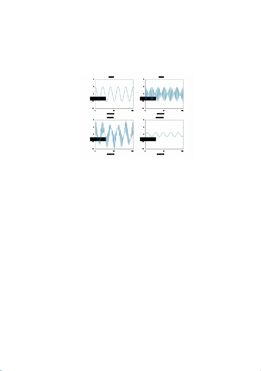
Q2.2 Program P2_1 is modified to simulate the LTI system y[n] = 0.5(x[n]x[n
1]) and process the input x[n] = s1[n]+s2[n] resulting in the output
sequence shown below:
2
The effect of changing the LTI system on the input is -
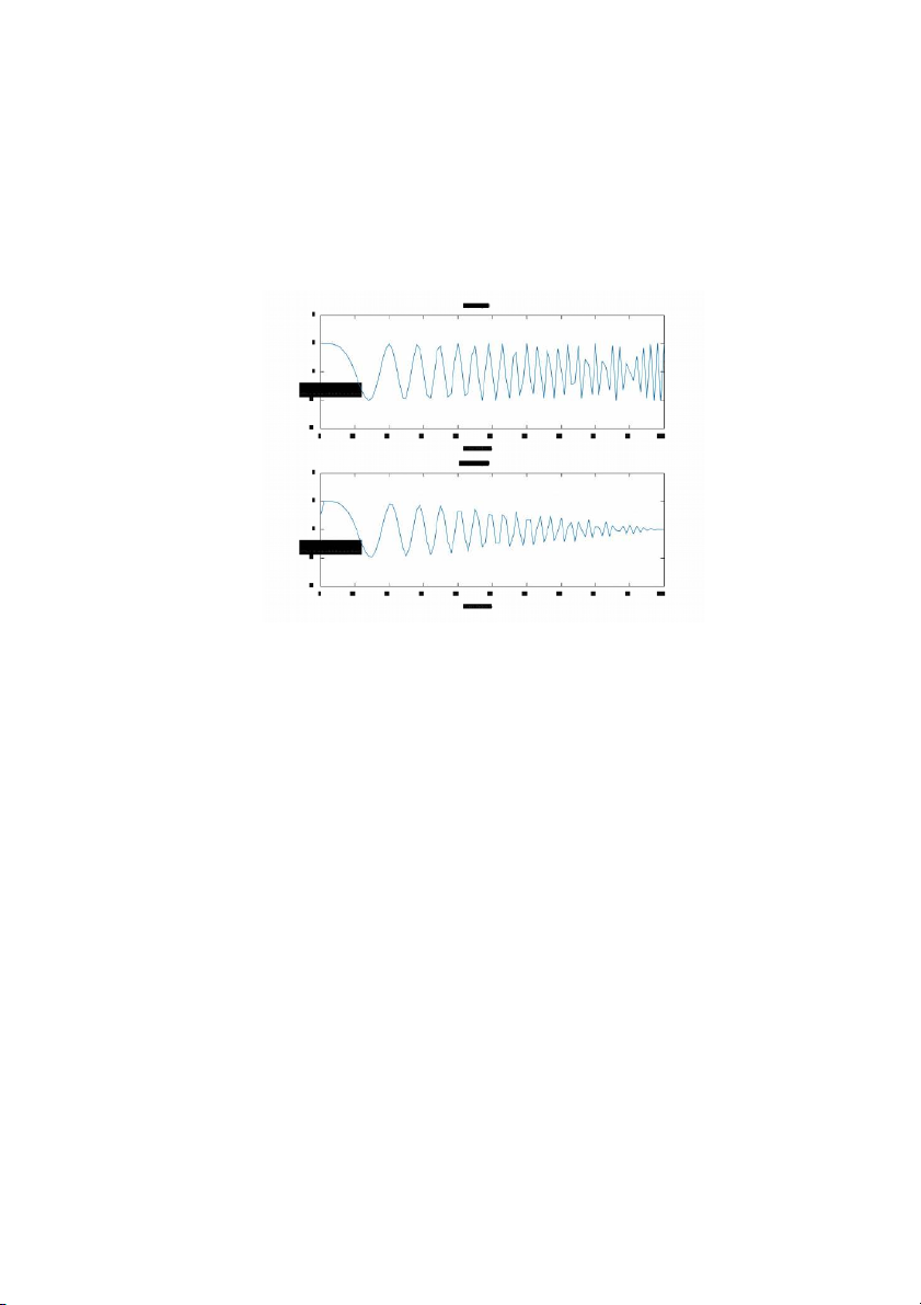
Q2.3 Program P2_1 is run for the following values of filter length M and following values
of the frequencies of the sinusoidal signals s1[n] and s2[n].The output
generated for these different values of M and the frequencies are shown
below.From these plots we make the following observations -
Q2.4 The required modifications to Program P2_1 by changing the input sequence to a
swept-frequency sinusoidal signal (length 101, minimum frequency 0, and a
maximum frequency 0.5) as the input signal (see Program P1_7) are listed below:
(a=pi/200, b=0)
% Program P2_1
% Simulation of an M-point Moving Average Filter
% Generate the input swept-frequency sinesoidal signal
%length 101, fmin=0 && fmax=0.5 --> a=pi/200, b=0;
n = 0:100;
a =pi/200; b=0;
arg = a*n.*n + b*n;
x = cos(arg);
% Implementation of the moving average filter
M=2;
num = ones(1,M);
y = filter(num,1,x)/M;
% Display the input and output signals
clf;
subplot(2,1,1);
plot(n, x);
axis([0, 100, -2, 2]);
xlabel( );'Time index n'); ylabel('Amplitude'
title( );'Input Signal'
subplot(2,1,2);
plot(n, y);
3
axis([0, 100, -2, 2]);
xlabel( );'Time index n'); ylabel('Amplitude'
title('Output Signal');
axis;
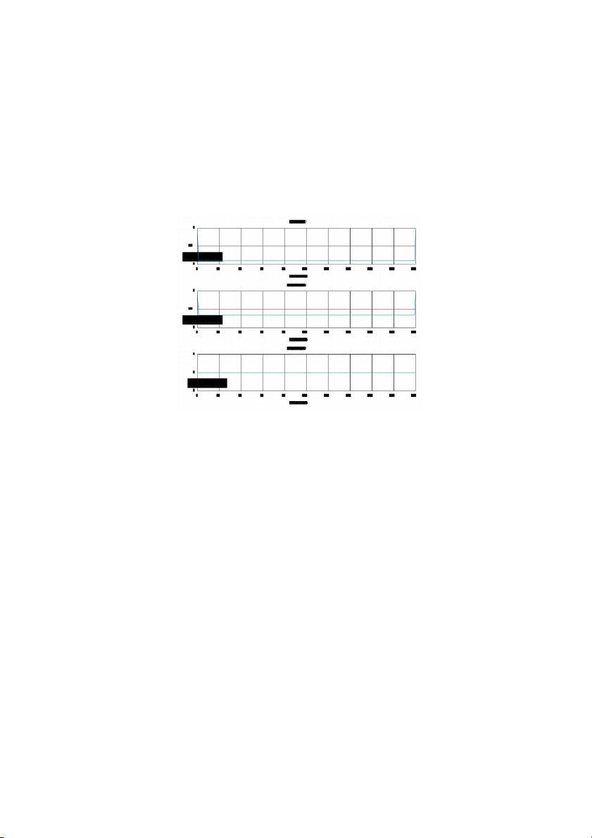
The output signal generated by running this program is plotted below.
The results of Questions Q2.1 and Q2.2 from the response of this system to the
swept-frequency signal can be explained as follows:
Project 2.2 (Optional) A Simple Nonlinear Discrete-Time System
% Program P2_2
% Generate a sinusoidal input signal
clf;
n = 0:200;
x = cos(2*pi*0.05*n);
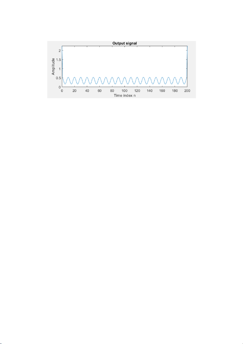
% Compute the output signal
x1 = [x 0 0]; % x1[n] = x[n+1]
x2 = [0 x 0]; % x2[n] = x[n]
x3 = [0 0 x]; % x3[n] = x[n-1]
y = x2.*x2-x1.*x3;
y = y(2:202);
% Plot the input and output signals
subplot(2,1,1)
plot(n, x)
xlabel('Time index n');ylabel( );'Amplitude'
title( )'Input Signal'
4
subplot(2,1,2)
plot(n,y)
xlabel('Time index n');ylabel( );'Amplitude'
title( );'Output signal'
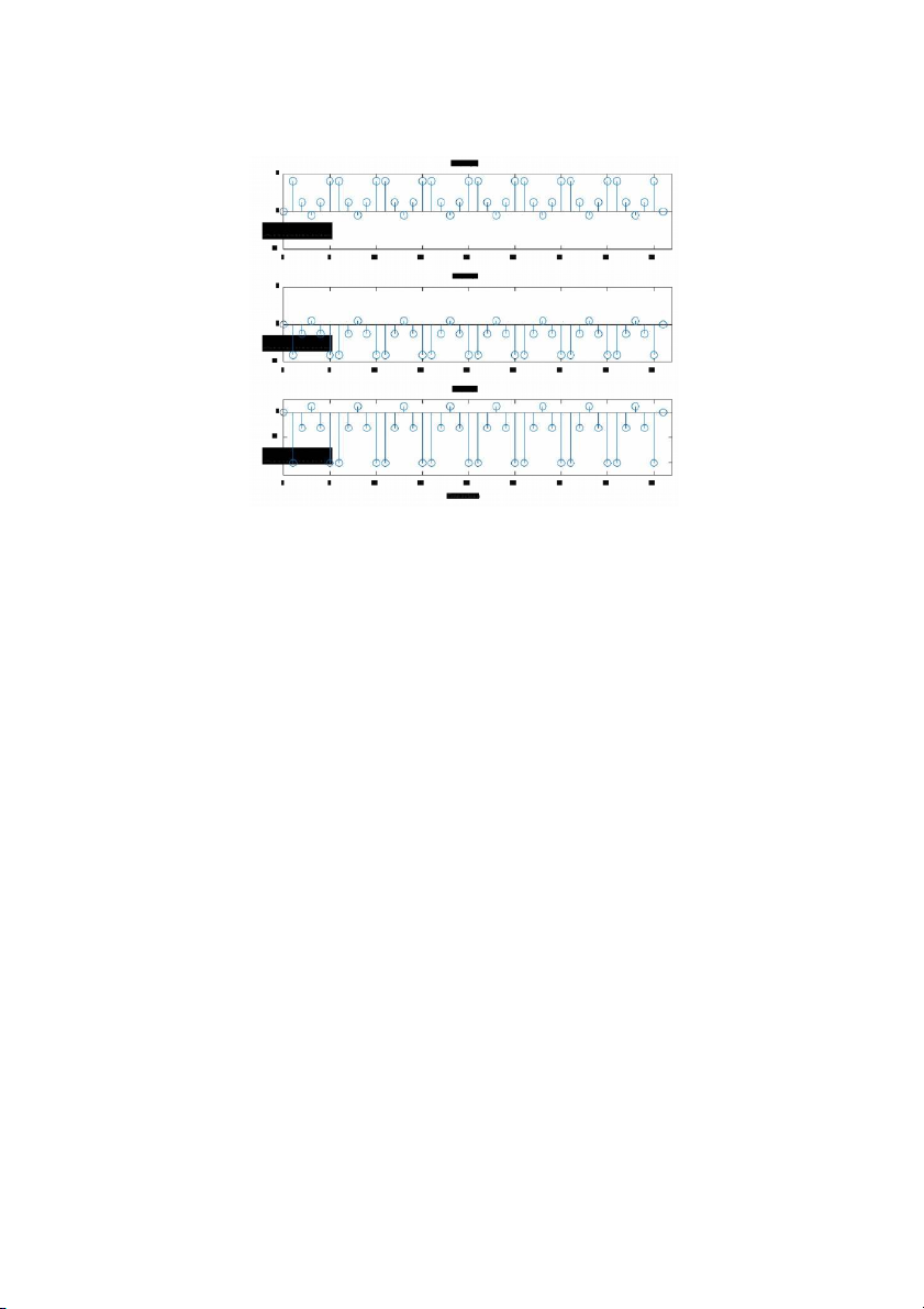
Q2.5 The sinusoidal signals with the following frequencies as the input signals were
used to generate the output signals:
The output signals generated for each of the above input signals are displayed
below:
The output signals depend on the frequencies of the input signal according to the following
rules:
This observation can be explained mathematically as follows: Give 2 frequencies fa
and fb. If fb is times fa c times the amplitude at fb is 2c times the amplitude at fa.
Q2.6 The output signal generated by using sinusoidal signals of the form x[n] =
sin(
o
n) + K as the input signal is shown below for the following values of
o
and K - w0 = 0.2 & K=0.5
5
The dependence of the output signal yt[n] on the DC value K can be explained as -
Project 2.3 Linear and Nonlinear Systems
% Program P2_3
% Generate the input sequences
clf;
n = 0:40;
a = 2;b = -3;
x1 = cos(2*pi*0.1*n);
x2 = cos(2*pi*0.4*n);
x = a*x1 + b*x2;
num = [2.2403 2.4908 2.2403];
den = [1 -0.4 0.75];
ic = [0 0]; % Set zero initial conditions
y1 = filter(num,den,x1,ic); % Compute the output y1[n]
y2 = filter(num,den,x2,ic); % Compute the output y2[n]
y = filter(num,den,x,ic); % Compute the output y[n]
yt = a*y1 + b*y2;
d = y - yt; % Compute the difference output d[n]
% Plot the outputs and the difference signal
subplot(3,1,1)
stem(n,y);
ylabel( );'Amplitude'
title('Output Due to Weighted Input: a \cdot x_{1}[n] + b \cdot x_{2}[n]');
subplot(3,1,2)
stem(n,yt);
ylabel( );'Amplitude'
title('Weighted Output: a \cdot y_{1}[n] + b \cdot y_{2}[n]');
subplot(3,1,3)
stem(n,d);
xlabel('Time index n');ylabel( );'Amplitude'
title('Difference Signal');
6
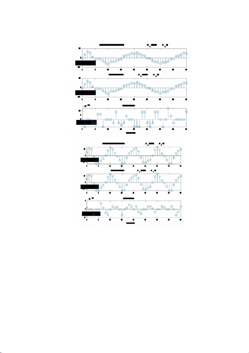
Q2.7 The outputs y[n], obtained with weighted input, and yt[n], obtained by
combining the two outputs y1[n] and y2[n] with the same weights, are shown
below along with the difference between the two signals:
The two sequences are - the same up numerical roundoff
The system is - Linear
Q2.8 Program P2_3 was run for the following three different sets of values of the
weighting constants, a and b, and the following three different sets of input
frequencies:
1. a=1; b=-1; f1=0.05; f2=0.4;
2. a=10; b=2; f1=0.10; f2=0.25;
3. a=2; b=10; f1=0.15; f2=0.20;
7
8
Based on these plots we can conclude that the system with different weights is -
Linear
Q2.9 Program 2_3 was run with the following non-zero initial conditions -
The plots generated are shown below -
Based on these plots we can conclude that the system with nonzero initial conditions is -
NonLinear
9
Q2.10 Program P2_3 was run with nonzero initial conditions and for the following three
different sets of values of the weighting constants, a and b, and the following
three different sets of input frequencies:
1. a=1; b=-1; f1=0.05; f2=0.4;
2. a=10; b=2; f1=0.10; f2=0.25;
3. a=2; b=10; f1=0.15; f2=0.20;
10
Based on these plots we can conclude that the system with nonzero initial
conditions and different weights is - NonLinear
Q2.11 Program P2_3 was modified to simulate the system:
y[n] = x[n]x[n1]
The output sequences y1[n], y2[n],and y[n]of the above system generated
by running the modified program are shown below:
11
Comparing y[n] with yt[n] we conclude that the two sequences are - Not the same
This system is - NonLinear
Project 2.4 Time-invariant and Time-varying Systems
A copy of Program P2_4 is given below:
% Program P2_4
% Generate the input sequences
clf;
n = 0:40; D = 10;a = 3.0;b = -2;
x = a*cos(2*pi*0.1*n) + b*cos(2*pi*0.4*n);
xd = [zeros(1,D) x];
num = [2.2403 2.4908 2.2403];
den = [1 -0.4 0.75];
ic = [0 0]; % Set initial conditions
% Compute the output y[n]
y = filter(num,den,x,ic);
% Compute the output yd[n]
yd = filter(num,den,xd,ic);
% Compute the difference output d[n]
d = y - yd(1+D:41+D);
% Plot the outputs
subplot(3,1,1)
stem(n,y);
ylabel('Amplitude');
12
title('Output y[n]'); grid;
subplot(3,1,2)
stem(n,yd(1:41));
ylabel( );'Amplitude'
title(['Output due to Delayed Input x[n Ð', num2str(D),']']); grid;
subplot(3,1,3)
stem(n,d);
xlabel('Time index n'); ylabel('Amplitude');
title('Difference Signal'); grid;
Q2.12 The output sequences y[n] and yd[n-10] generated by running Program P2_4
are shown below -
These two sequences are related as follows - yd[n] = y[n-10]
The system is - Time Invariant
Q2.13 The output sequences y[n] and yd[n-D] generated by running Program P2_4 for
the following values of the delay variable D - 2,6,8 are shown below -
13
14
In each case, these two sequences are related as follows - y[n-D]=yd[n]
The system is - Time Invariant
Q2.14 The output sequences y[n] and yd[n-10] generated by running Program P2_4
for the following values of the input frequencies -
1. f1=0.05; f2=0.40;
2. f1=0.10; f2=0.25;
3. F1=0.15; f2=0.2
15
In each case, these two sequences are related as follows - y[n-10]=yd[n]
The system is - Time Invariant
Q2.15 The output sequences y[n] and yd[n-10] generated by running Program P2_4
for non-zero initial conditions are shown below -
These two sequences are related as follows - yd[n] is NOT equal to the shift of y[n].
16
The system is - Time Varying
Q2.16 The output sequences y[n] and yd[n-10] generated by running Program P2_4
for non-zero initial conditions and following values of the input frequencies -
1. f1=0.05; f2=0.40;
2. f1=0.10; f2=0.25;
3. f1=0.15; f2=0.20;
17
In each case, these two sequences are related as follows - yd[n] is NOT given by
the shift of y[n].
The system is - Time Varying
Q2.17 The modified Program 2_4 simulating the system
y[n] = n x[n] + x[n-1]
% Program Q2_17
% Modification of P2_4 to implement the system
% given by (2.16).
% Generate the input sequences
clf;
n = 0:40; D = 10;a = 3.0;b = -2;
x = a*cos(2*pi*0.1*n) + b*cos(2*pi*0.4*n);
xd = [zeros(1,D) x];
nd = 0:length(xd)-1;
% Compute the output y[n]
y = (n .* x) + [0 x(1:40)];
% Compute the output yd[n]
yd = (nd .* xd) + [0 xd(1:length(xd)-1)];
% Compute the difference output d[n]
d = y - yd(1+D:41+D);
% Plot the outputs
subplot(3,1,1)
stem(n,y);
ylabel( );'Amplitude'
18
title('Output y[n]'); grid;
subplot(3,1,2)
stem(n,yd(1:41));
ylabel( );'Amplitude'
title(['Output due to Delayed Input x[n -',
num2str(D),']']); grid;
subplot(3,1,3)
stem(n,d);
xlabel( );'Time index n'); ylabel('Amplitude'
title('Difference Signal'); grid;
The output sequences y[n] and yd[n-10] generated by running modified
Program P2_4 are shown below -
These two sequences are related as follows - Not the same
The system is - Nonlinear
Q2.18 (optional) The modified Program P2_3 to test the linearity of the system of Q2.18 is
shown below:
% Program Q2_18
% Generate the input sequences
clf;
n = 0:40;
a = 2;b = -3;
x1 = cos(2*pi*0.1*n);
x2 = cos(2*pi*0.4*n);
x = a*x1 + b*x2;
y1 = (n .* x1) + [0 x1(1:40)]; % Compute the output y1[n]
19
y2 = (n .* x2) + [0 x2(1:40)]; % Compute the output y2[n]
y = (n .* x) + [0 x(1:40)]; % Compute the output y[n]
yt = a*y1 + b*y2;
d = y - yt; % Compute the difference output d[n]
% Plot the outputs and the difference signal
subplot(3,1,1)
stem(n,y);
ylabel( );'Amplitude'
title('Output Due to Weighted Input: a \cdot x_{1}[n] + b
\cdotx_{2}[n]');
subplot(3,1,2)
stem(n,yt);
ylabel( );'Amplitude'
title('Weighted Output: a \cdot y_{1}[n] + b \cdot y_{2}
[n]');
subplot(3,1,3)
stem(n,d);
xlabel( );ylabel( );'Time index n' 'Amplitude'
title( );'Difference Signal'
The outputs y[n]and yt[n] obtained by running the modified program P2_3 are
shown below:
The two sequences are - The same
- LinearThe system is
20
| 1/35

Preview text:

Name: Phm Th ị H n ươ g Gi a ng 1 8 1 6 1 0 6 8 Anh Đ c 1 8 1 6 1 0 6 2 Section: Gr o up 2 La bo r a t o r y Ex e r c i s e 2 DI SCRETE- TI ME S YS TEMS: TI ME- DOMAI N REPRESENTATI ON 2.1
SIMULATION OF DISCRETE-TIME SYSTEMS Project 2.1
The Moving Average System % Program P2_1
% Simulation of an M-point Moving Average Filter % Generate the input signal n = 0:100;
s1 = cos(2*pi*0.05*n); % A low-frequency sinusoid
s2 = cos(2*pi*0.47*n); % A high frequency sinusoid x = s1+s2;
% Implementation of the moving average filter
M = input('Desired length of the filter = '); num = ones(1,M); y = filter(num,1,x)/M;
% Display the input and output signals clf; subplot(2,2,1); plot(n, s1); axis([0, 100, -2, 2]);
xlabel('Time index n'); ylabel('Amplitude'); title('Signal #1'); subplot(2,2,2); plot(n, s2); axis([0, 100, -2, 2]);
xlabel('Time index n'); ylabel('Amplitude'); title('Signal #2'); subplot(2,2,3); plot(n, x); axis([0, 100, -2, 2]);
xlabel('Time index n'); ylabel('Amplitude'); title( ); 'Input Signal' subplot(2,2,4); plot(n, y); axis([0, 100, -2, 2]);
xlabel('Time index n'); ylabel('Amplitude'); title('Output Signal'); 1 axis; Q2.1
The output sequence generated by running the above program for M = 2 with x[n] = s1[n]+s2[n] as the input is shown below.
The component of the input x[n] suppressed by the discrete-time system simulated by this program is - S i g n a l # 2 , i t i s a h i g h f r e q u e n c y s i g n a l a n d b e s u p p r e s s e d b y a l o w p a s s fil t e r s y s t e m. Q2.2
Program P2_1 is modified to simulate the LTI system y[n] = 0.5(x[n]–x[n–
1]) and process the input x[n] = s1[n]+s2[n] resulting in the output sequence shown below: 2
The effect of changing the LTI system on the input is - Q2.3
Program P2_1 is run for the following values of filter length M and following values
of the frequencies of the sinusoidal signals s1[n] and s2[n].The output
generated for these different values of M and the frequencies are shown
below.From these plots we make the following observations - Q2.4
The required modifications to Program P2_1 by changing the input sequence to a
swept-frequency sinusoidal signal (length 101, minimum frequency 0, and a
maximum frequency 0.5) as the input signal (see Program P1_7) are listed below : ( a =p i / 2 0 0 , b =0 ) % Program P2_1
% Simulation of an M-point Moving Average Filter
% Generate the input swept-frequency sinesoidal signal
%length 101, fmin=0 && fmax=0.5 --> a=pi/200, b=0; n = 0:100; a =pi/200; b=0; arg = a*n.*n + b*n; x = cos(arg);
% Implementation of the moving average filter M=2; num = ones(1,M); y = filter(num,1,x)/M;
% Display the input and output signals clf; subplot(2,1,1); plot(n, x); axis([0, 100, -2, 2]);
xlabel('Time index n'); ylabel('Amplitude'); title( ); 'Input Signal' subplot(2,1,2); plot(n, y); 3 axis([0, 100, -2, 2]);
xlabel('Time index n'); ylabel('Amplitude'); title('Output Signal'); axis;
The output signal generated by running this program is plotted below.
The results of Questions Q2.1 and Q2.2 from the response of this system to the
swept-frequency signal can be explained as follows: Project 2.2
(Optional) A Simple Nonlinear Discrete-Time System % Program P2_2
% Generate a sinusoidal input signal clf; n = 0:200; x = cos(2*pi*0.05*n); % Compute the output signal
x1 = [x 0 0]; % x1[n] = x[n+1] x2 = [0 x 0]; % x2[n] = x[n] x3 = [0 0 x]; % x3[n] = x[n-1] y = x2.*x2-x1.*x3; y = y(2:202);
% Plot the input and output signals subplot(2,1,1) plot(n, x) xlabel('Time index n');ylabel( ); 'Amplitude' title('Input Signal') 4 subplot(2,1,2) plot(n,y) xlabel('Time index n');ylabel( ); 'Amplitude' title('Output signal'); Q2.5
The sinusoidal signals with the following frequencies as the input signals were
used to generate the output signals:
The output signals generated for each of the above input signals are displayed below:
The output signals depend on the frequencies of the input signal according to the following rules:
This observation can be explained mathematically as follows: Gi v e 2 f r e q u e n c i e s f a a n d f b . I f f b i s t i me s f a c t i me s t h e a mp l i t u d e a t f b i s 2 c t i me s t h e a mp l i t u d e a t f a . Q2.6
The output signal generated by using sinusoidal signals of the form x[n] = sin( on) + K
as the input signal is shown below for the following values of o and K - w0 = 0 . 2 & K=0 . 5 5
The dependence of the output signal yt[n] on the DC value K can be explained as - Project 2.3
Linear and Nonlinear Systems % Program P2_3 % Generate the input sequences clf; n = 0:40; a = 2;b = -3; x1 = cos(2*pi*0.1*n); x2 = cos(2*pi*0.4*n); x = a*x1 + b*x2; num = [2.2403 2.4908 2.2403]; den = [1 -0.4 0.75];
ic = [0 0]; % Set zero initial conditions
y1 = filter(num,den,x1,ic); % Compute the output y1[n]
y2 = filter(num,den,x2,ic); % Compute the output y2[n]
y = filter(num,den,x,ic); % Compute the output y[n] yt = a*y1 + b*y2;
d = y - yt; % Compute the difference output d[n]
% Plot the outputs and the difference signal subplot(3,1,1) stem(n,y); ylabel('Amplitude');
title('Output Due to Weighted Input: a \cdot x_{1}[n] + b \cdot x_{2}[n]'); subplot(3,1,2) stem(n,yt); ylabel('Amplitude');
title('Weighted Output: a \cdot y_{1}[n] + b \cdot y_{2}[n]'); subplot(3,1,3) stem(n,d); xlabel('Time index n');ylabel( ); 'Amplitude' title('Difference Signal'); 6 Q2.7
The outputs y[n], obtained with weighted input, and yt[n], obtained by
combining the two outputs y1[n] and y2[n] with the same weights, are shown
below along with the difference between the two signals: The two sequences are - t h e s a me u p n u me r i c a l r o u n d o ff The system is - Li n e a r Q2.8
Program P2_3 was run for the following three different sets of values of the
weighting constants, a and b, and the following three different sets of input frequencies: 1 . a=1; b=-1; f1=0.05; f2=0.4;
2. a=10; b=2; f1=0.10; f2=0.25;
3. a=2; b=10; f1=0.15; f2=0.20; 7 8
Based on these plots we can conclude that the system with different weights is - Linear Q2.9
Program 2_3 was run with the following non-zero initial conditions -
The plots generated are shown below -
Based on these plots we can conclude that the system with nonzero initial conditions is - NonLinear 9
Q2.10 Program P2_3 was run with nonzero initial conditions and for the following three
different sets of values of the weighting constants, a and b, and the following
three different sets of input frequencies: 1 . a=1; b=-1; f1=0.05; f2=0.4;
2. a=10; b=2; f1=0.10; f2=0.25;
3. a=2; b=10; f1=0.15; f2=0.20; 1 0
Based on these plots we can conclude that the system with nonzero initial
conditions and different weights is - No n Li n e a r
Q2.11 Program P2_3 was modified to simulate the system: y[n] = x[n]x[n–1] The output sequences y1[n], y2[n],and
y[n]of the above system generated
by running the modified program are shown below: 1 1 Comparing y[n] with
yt[n] we conclude that the two sequences are - No t t h e s a me This system is - No n Li n e a r Project 2.4
Time-invariant and Time-varying Systems
A copy of Program P2_4 is given below: % Program P2_4 % Generate the input sequences clf;
n = 0:40; D = 10;a = 3.0;b = -2;
x = a*cos(2*pi*0.1*n) + b*cos(2*pi*0.4*n); xd = [zeros(1,D) x]; num = [2.2403 2.4908 2.2403]; den = [1 -0.4 0.75];
ic = [0 0]; % Set initial conditions % Compute the output y[n] y = filter(num,den,x,ic); % Compute the output yd[n] yd = filter(num,den,xd,ic);
% Compute the difference output d[n] d = y - yd(1+D:41+D); % Plot the outputs subplot(3,1,1) stem(n,y); ylabel('Amplitude'); 1 2 title('Output y[n]'); grid; subplot(3,1,2) stem(n,yd(1:41)); ylabel('Amplitude');
title(['Output due to Delayed Input x[n Ð', num2str(D),']']); grid; subplot(3,1,3) stem(n,d);
xlabel('Time index n'); ylabel('Amplitude');
title('Difference Signal'); grid;
Q2.12 The output sequences y[n] and
yd[n-10] generated by running Program P2_4 are shown below -
These two sequences are related as follows - y d [ n ] = y [ n - 1 0 ] The system is - Ti me I n v a r i a n t Q sequ2 nces . 13 y Th [e out putn] and
yd[n-D] generated by running Program P2_4 for
the following values of the delay variable D - 2 , 6 , 8 are shown below - 1 3 1 4
In each case, these two sequences are related as follows - y [ n - D] =y d [ n ] The system is - Ti me I n v a r i a n t
Q2.14 The output sequences y[n] and
yd[n-10] generated by running Program P2_4
for the following values of the input frequencies - 1. f1=0.05; f2=0.40; 2. f1=0.10; f2=0.25; 3. F1=0.15; f2=0.2 1 5
In each case, these two sequences are related as follows - y [ n - 1 0 ] =y d [ n ] The system is - Ti me I n v a r i a n t
Q2.15 The output sequences y[n] and
yd[n-10] generated by running Program P2_4
for non-zero initial conditions are shown below -
These two sequences are related as follows -
yd[n] is NOT equal to the shift of y[n]. 1 6 The system is - Ti me Va r y i n g
Q2.16 The output sequences y[n] and
yd[n-10] generated by running Program P2_4
for non-zero initial conditions and following values of the input frequencies - 1. f1=0.05; f2=0.40; 2. f1=0.10; f2=0.25; 3. f1=0.15; f2=0.20; 1 7
In each case, these two sequences are related as follows - yd[n] is NOT given by the shift of y[n]. The system is - Ti me Va r y i n g Q2.17
The modified Program 2_4 simulating the system y[n] = n x[n] + x[n-1] % Program Q2_17
% Modification of P2_4 to implement the system % given by (2.16). % Generate the input sequences clf;
n = 0:40; D = 10;a = 3.0;b = -2;
x = a*cos(2*pi*0.1*n) + b*cos(2*pi*0.4*n); xd = [zeros(1,D) x]; nd = 0:length(xd)-1; % Compute the output y[n] y = (n .* x) + [0 x(1:40)]; % Compute the output yd[n]
yd = (nd .* xd) + [0 xd(1:length(xd)-1)];
% Compute the difference output d[n] d = y - yd(1+D:41+D); % Plot the outputs subplot(3,1,1) stem(n,y); ylabel('Amplitude'); 1 8 title('Output y[n]'); grid; subplot(3,1,2) stem(n,yd(1:41)); ylabel('Amplitude');
title(['Output due to Delayed Input x[n -', num2str(D),']']); grid; subplot(3,1,3) stem(n,d);
xlabel('Time index n'); ylabel('Amplitude');
title('Difference Signal'); grid; The output sequences y[n] and
yd[n-10] generated by running modified Program P2_4 are shown below -
These two sequences are related as follows - No t t h e s a me The system is - No n l i n e a r
Q2.18 (optional) The modified Program P2_3 to test the linearity of the system of Q2.18 is shown below: % Program Q2_18 % Generate the input sequences clf; n = 0:40; a = 2;b = -3; x1 = cos(2*pi*0.1*n); x2 = cos(2*pi*0.4*n); x = a*x1 + b*x2;
y1 = (n .* x1) + [0 x1(1:40)]; % Compute the output y1[n] 1 9
y2 = (n .* x2) + [0 x2(1:40)]; % Compute the output y2[n]
y = (n .* x) + [0 x(1:40)]; % Compute the output y[n] yt = a*y1 + b*y2;
d = y - yt; % Compute the difference output d[n]
% Plot the outputs and the difference signal subplot(3,1,1) stem(n,y); ylabel('Amplitude');
title('Output Due to Weighted Input: a \cdot x_{1}[n] + b \cdotx_{2}[n]'); subplot(3,1,2) stem(n,yt); ylabel('Amplitude');
title('Weighted Output: a \cdot y_{1}[n] + b \cdot y_{2} [n]'); subplot(3,1,3) stem(n,d); xlabel( );ylabel( 'Time index n' 'Amplitude'); title('Difference Signal');
The outputs y[n]and yt[n] obtained by running the modified program P2_3 are shown below: The two sequences are - Th e s a me The system is - Li n e a r 2 0