Mẫu số chuyên môn bệnh viện : 47 loại | Đạo học Hoa Sen

1.1
Systems of linear algebraic equations and their solutions constitute one of the INTRODUCTION TO
major topics studied in the course known as “linear algebra.” In this first section
we shall introduce some basic terminology and discuss a method for solving such SYSTEMS OF LINEAR systems. EQUATIONS Linear Equations Any straight line in the
-plane can be represented algebraically by an equation of the form where ,
, and b are real constants and and
are not both zero. An equation of this form is called a linear equation in the
variables x and y. More generally, we define a linear equatio
n in the n variables , , …,
to be one that can be expressed in the form where , , …,
, and b are real constants. The variables in a linear equation are sometimes called unknowns.
EXAMPLE 1 Linear Equations The equations
are linear. Observe that a linear equation does not involve any products or roots of variables. All variables occur only to the first
power and do not appear as arguments for trigonometric, logarithmic, or exponential functions. The equations are not linear.
A solution of a linear equation
is a sequence of n numbers , , …, such that the equation is satisfied when we substitute , , …,
. The set of all solutions of the equation is called its solution set or
sometimes the general solution of the equation.
EXAMPLE 2 Finding a Solution Set Find the solution set of (a) , and (b) . Solution (a)
To find solutions of (a), we can assign an arbitrary value to x and solve for y, or choose an arbitrary value for y and solve for x. If
we follow the first approach and assign x an arbitrary value t, we obtain
These formulas describe the solution set in terms of an arbitrary number t, called a parameter. Particular numerical solutions can be
obtained by substituting specific values for t. For example, yields the solution , ; and yields the solution , .
If we follow the second approach and assign y the arbitrary value t, we obtain
Although these formulas are different from those obtained above, they yield the same solution set as t varies over all possible real
numbers. For example, the previous formulas gave the solution , when
, whereas the formulas immediately above yield that solution when . Solution (b)
To find the solution set of (b), we can assign arbitrary values to any two variables and solve for the third variable. In particular, if
we assign arbitrary values s and t to and , respectively, and solve for , we obtain Linear Systems
A finite set of linear equations in the variables , , …,
is called a system of linear equations or a linear system. A sequence
of numbers , , …, is called a solution of the system if , , …,
is a solution of every equation in the
system. For example, the system has the solution , ,
since these values satisfy both equations. However, , , is not a
solution since these values satisfy only the first equation in the system.
Not all systems of linear equations have solutions. For example, if we multiply the second equation of the system
by , it becomes evident that there are no solutions since the resulting equivalent system has contradictory equations.
A system of equations that has no solutions is said to be inconsistent; if there is at least one solution of the system, it is called
consistent. To illustrate the possibilities that can occur in solving systems of linear equations, consider a general system of two
linear equations in the unknowns x and y:
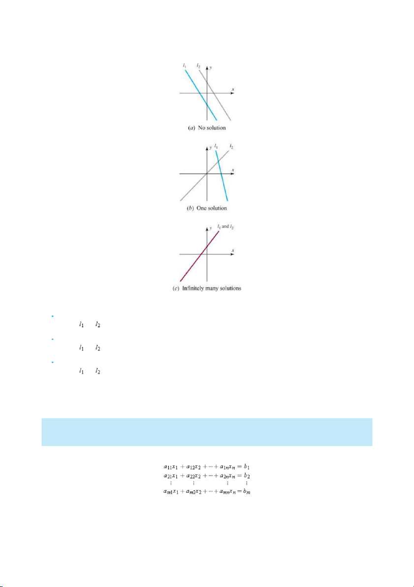
The graphs of these equations are lines; call them and . Since a point (x, y) lies on a line if and only if the numbers x and y
satisfy the equation of the line, the solutions of the system of equations correspond to points of intersection of and . There are
three possibilities, illustrated in Figure 1.1.1: Figure 1.1.1
The lines and may be parallel, in which case there is no intersection and consequently no solution to the system.
The lines and may intersect at only one point, in which case the system has exactly one solution.
The lines and may coincide, in which case there are infinitely many points of intersection and consequently infinitely many solutions to the system.
Although we have considered only two equations with two unknowns here, we will show later that the same three possibilities hold for arbitrary linear systems:
Every system of linear equations has no solutions, or has exactly one solution, or has infinitely many solutions.
An arbitrary system of m linear equations in n unknowns can be written as where , , …,
are the unknowns and the subscripted a's and b's denote constants. For example, a general system of three
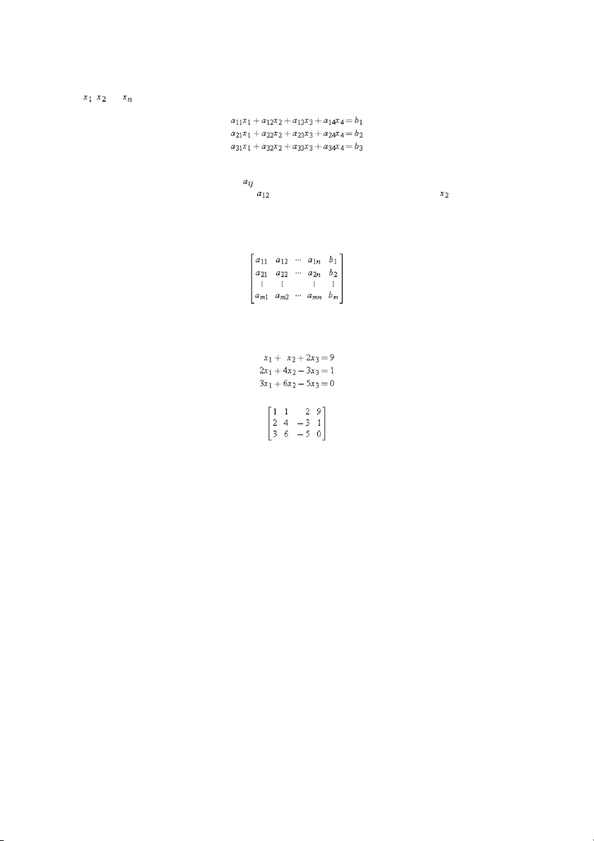
linear equations in four unknowns can be written as
The double subscripting on the coefficients of the unknowns is a useful device that is used to specify the location of the coefficient
in the system. The first subscript on the coefficient
indicates the equation in which the coefficient occurs, and the second
subscript indicates which unknown it multiplies. Thus,
is in the first equation and multiplies unknown . Augmented Matrices
If we mentally keep track of the location of the +'s, the x's, and the ='s, a system of m linear equations in n unknowns can be
abbreviated by writing only the rectangular array of numbers:
This is called the augmented matrix for the system. (The term matrix is used in mathematics to denote a rectangular array of
numbers. Matrices arise in many contexts, which we will consider in more detail in later sections.) For example, the augmented
matrix for the system of equations is
Remark When constructing an augmented matrix, we must write the unknowns in the same order in each equation, and the
constants must be on the right.
The basic method for solving a system of linear equations is to replace the given system by a new system that has the same solution
set but is easier to solve. This new system is generally obtained in a series of steps by applying the following three types of
operations to eliminate unknowns systematically:
1. Multiply an equation through by a nonzero constant. 2. Interchange two equations.
3. Add a multiple of one equation to another.
Since the rows (horizontal lines) of an augmented matrix correspond to the equations in the associated system, these three
operations correspond to the following operations on the rows of the augmented matrix:
1. Multiply a row through by a nonzero constant. 2. Interchange two rows.
3. Add a multiple of one row to another row. Elementary Row Operations
These are called elementary row operations. The following example illustrates how these operations can be used to solve systems
of linear equations. Since a systematic procedure for finding solutions will be derived in the next section, it is not necessary to
worry about how the steps in this example were selected. The main effort at this time should be devoted to understanding the
computations and the discussion.
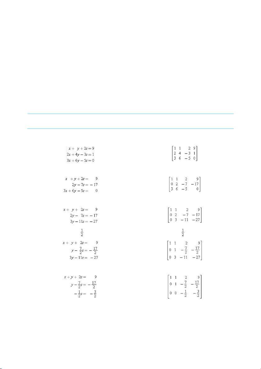
EXAMPLE 3 Using Elementary Row Operations
In the left column below we solve a system of linear equations by operating on the equations in the system, and in the right column
we solve the same system by operating on the rows of the augmented matrix.
Add −2 times the first equation to the second to obtain
Add −2 times the first row to the second to obtain
Add −3 times the first equation to the third to obtain
Add −3 times the first row to the third to obtain
Multiply the second equation by to obtain
Multiply the second row by to obtain
Add −3 times the second equation to the third to obtain
Add −3 times the second row to the third to obtain
Multiply the third equation by − 2 to obtain
Multiply the third row by −2 to obtain
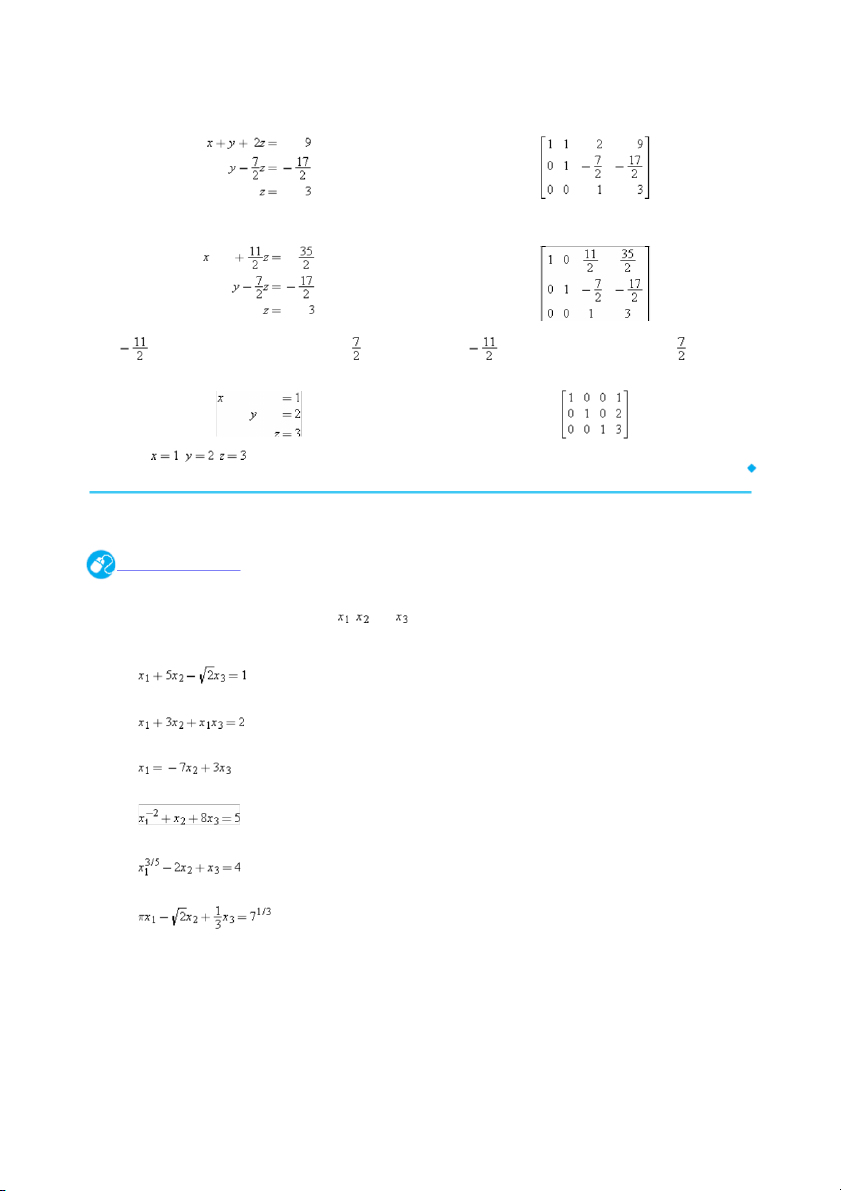
Add −1 times the second equation to the first to obtain
Add −1 times the second row to the first to obtain Add
times the third equation to the first and times the Add
times the third row to the first and times the
third equation to the second to obtain
third row to the second to obtain The solution , , is now evident. Exercise Set 1.1 Click here for Just Ask!
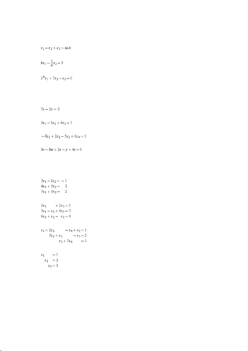
Which of the following are linear equations in , , and ? 1. (a) (b) (c) (d) (e) (f)
Given that k is a constant, which of the following are linear equations? 2. (a) (b) (c)
Find the solution set of each of the following linear equations. 3. (a) (b) (c) (d)
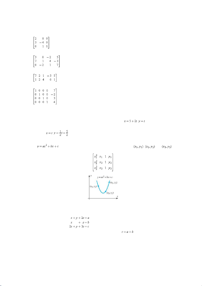
Find the augmented matrix for each of the following systems of linear equations. 4. (a) (b) (c) (d)
Find a system of linear equations corresponding to the augmented matrix. 5. (a) (b) (c) (d) 6.
(a) Find a linear equation in the variables x and y that has the general solution , . (b) Show that ,
is also the general solution of the equation in part (a). The curve
shown in the accompanying figure passes through the points , , and . Show
7. that the coefficients a, b, and c are a solution of the system of linear equations whose augmented matrix is Figure Ex-7
Consider the system of equations 8.
Show that for this system to be consistent, the constants a, b, and c must satisfy .