Petri Nets: Chapter overview and applications môn FMS & CIM | Trường Đại học Bách Khoa Hà Nội
Petri nets were introduced in 1962 by Dr. Carl Adam Petri (Petri 1962). Petri nets are a powerful modeling formalism in computer science, system engineering and many other disciplines. Tài liệu được sưu tầm gồm 19 trang, giúp các bạn ôn luyện và phục vụ cho việc học tập, đạt kết quả tốt. Mời các bạn đón xem!
Môn: FMS & CIM 12 tài liệu
Trường: Đại học Bách Khoa Hà Nội 5.8 K tài liệu
Tác giả:


Preview text:
See discussions, stats, and author profiles for this publication at: https://www.researchgate.net/publication/334339931 Petri Nets Chapter · June 2019 DOI: 10.1201/9780429184185-8 CITATIONS READS 0 3,623 William M. Tepfenhart Monmouth University
283 PUBLICATIONS 2,826 CITATIONS
61 PUBLICATIONS 550 CITATIONS SEE PROFILE
All content following this page was uploaded by Jiacun Wang on 24 May 2021.
The user has requested enhancement of the downloaded file.
In: Jiacun Wang, Handbook of finite state based models and applications, CRC Press, 2012
Chapter 15. Petri Nets Jiacun Wang
Department of Computer Science and Software Engineering Monmouth University
West Long Branch, NJ 07764 jwang@monmouth.edu 15.1 Introduction
Petri nets were introduced in 1962 by Dr. Carl Adam Petri (Petri 1962). Petri nets are a powerful modeling formalism
in computer science, system engineering and many other disciplines. Petri nets combine a well defined mathematical
theory with a graphical representation of the dynamic behavior of systems. The theoretic aspect of Petri nets allows
precise modeling and analysis of system behavior, while the graphical representation of Petri nets enables visualization
of the modeled system state changes. This combination is the main reason for the great success of Petri nets.
Consequently, Petri nets have been used to model various kinds of dynamic event-driven systems such as computers
networks (Ajmone Marsan, Balbo and Conte 1986), communication systems (Merlin and Farber 1976; Wang 2006),
manufacturing plants (Venkatesh, Zhou and Caudill 1994; Zhou and DiCesare 1989; Desrochers and Ai-Jaar 1995),
command and control systems (Andreadakis and Levis 1988), real-time computing systems (Mandrioli and Morzenti
1996; Tsai, Yang and Chang 1995), logistic networks (Landeghem and Bobeanu 2002), hybrid systems (Pettersson
and Lennartson, 1995), biological systems (Kitakaze, Matsuno and Ikeda 2006), and workflows (Aalst and Hee 2000;
Lin, Tian and Wei 2002) to mention only a few important examples. This wide spectrum of applications is
accompanied by wide spectrum different aspects which have been considered in the research on Petri nets.
15.2 Graphic Representation
15.2.1 Graphic Representation
A Petri net is a particular kind of bipartite directed graphs populated by four types of objects. These objects are places,
transitions, directed arcs and tokens. Directed arcs connect places to transitions or transitions to places. In its simplest
form, a Petri net can be represented by a transition together with an input place and an output place. This elementary
net may be used to represent various aspects of the modeled systems. For example, a transition and its input place and
output place can be used to represent a data processing event, its input data and output data, respectively, in a data
processing system. In order to study the dynamic behavior of a Petri net modeled system in terms of its states and state
changes, each place may potentially hold either none or a positive number of tokens. Tokens are a primitive concept
for Petri nets in addition to places and transitions. The presence or absence of a token in a place may indicate whether
a condition associated with this place is true or false, for instance. t 1 p 2 t 3 2 2 p 3 p 5 p 1 t 2 p 4 t 4
Fig. 15.1 A Petri net with 5 places and 4 transitions.
Most theoretical work on Petri nets is based on the formal definition of Petri nets. However, a graphical representation
of a Petri net is much more useful for illustrating the concepts of Petri net theory. A Petri net graph is a Petri net
depicted as a bipartite directed multigraph. Corresponding to the definition of Petri nets, a Petri net graph has two
types of nodes: a circle represents a place, and a bar or box represents a transition. Directed arcs (arrows) connect
places and transitions, with some arcs directed from places to transitions and other arcs directed from transitions to places.
The Petri net shown in Fig. 15.1 is composed of five places, namely p1, p2, p3, p4 and p5, and four transitions, namely
t1, t2, t3 and t4. p1 is an input place to t1 and t2 because there is one directed arc contacting p1 to t1 and another one
contacting p1 to t2. p3 and p4 are both output places to t2 because there is an arc from t2 to p3 and an arc from t2 to p4. p1
has one token, while all other places have 0 tokens. A directed arc can have a weight, which is labeled to the arc in the
graphic representation. The weight of the arc from t2 to p3 and arc from p3 to t3 is 2. The weight of all other arcs is 1, by default.
The execution of a Petri net is controlled by the number and distribution of tokens in the Petri net. By changing
distribution of tokens in places, which may reflect the occurrence of events or execution of operations, for instance,
one can study the dynamic behavior of the modeled system. A Petri net is executed by firing transitions. However,
only an enabled transition can fire.
A transition t is said to be enabled if each input place p of t contains at least the number of tokens equal to the weight
of the directed arc connecting p to t. For example, both transitions t1 and t2 are enabled in the Petri net of Fig. 15.1.
The firing of an enabled transition t removes from each input place p the number of tokens equal to the weight of the
arc from p to t, and deposits in each output place p the number of tokens equal to the weight of the arc from t to p. Fig.
15.2 shows the new token distribution of the Petri net of Fig. 15.1 after firing t2. t 1 p 2 t 3 2 2 p 5 p 1 p 3 t 2 p4 t4
Fig. 15.2 Firing of transition t2.
Places are passive elements, while transitions are active elements. In a practical system model, places represent buffers,
channels, geographical locations, conditions or states, transitions represent events, computation, transformation or
transportation. Tokens represent objects (e.g. humans, goods and machines), information, conditions or states of
objects. A system state is specified by token distribution in places, which is called a marking in Petri net language.
State transitions leading from one state to another are realized through transition firing.
Notice that since only enabled transitions can fire, the number of tokens in each place always remains non-negative
when a transition is fired. Firing a transition can never try to remove a token that is not there.
A transition without any input place is called a source transition, and one without any output place is called a sink
transition. Note that a source transition is unconditionally enabled, and that the firing of a sink transition consumes
tokens, but doesn’t produce tokens.
A pair of a place p and a transition t is called a self-loop, if p is both an input place and an output place of t. A
Petri net is said to be pure if it has no self-loops.
15.2.2 Modeling Example: A Reader-writer System
Fig. 15.3 shows the Petri net model of a classical reader-writer system. Initially, both the reader and writer are at rest
(places r_rest and w_rest each contains a token). Then the writer begins to write a mail (transition write fires, the token
in w_rest is removed and a token deposited into place mail). Now transition send is enabled and can fire. Firing send
removes the token from place mail and deposit a token to w_rest and a token to mail_box, meaning now the writer is
at rest again and one mail is in the mail box.
Since both mail_box and r_rest have a token, transition receive is enabled. Firing receive removes the token from
mail_box and r_rest and adds a token to place received. Now the mail_box is empty (no token in mail_box). After
reading a received mail, the reader is waiting to receive new mails from the mail box (transition read fires and a token
is added to place r_rest). write receive mail w_rest received r_rest mail_box send read
Fig. 15.3. A reader-writer system.
The above transition firing sequence write-send -receive -read brings the Petri net back to the initial marking, at which
place w_rest and r_rest each has a token and all other places have no tokens. However, after the firing of write and
send, these two transitions may fire again and again before the firing of receive. Each time write and send fire, one
token that represents a mail is added to place mail_box. Therefore, the model of Fig. 15.3 assumes the capacity of the
mail box is unlimited. How to model a mail box that can hold up to a limited number of mails? Well, to this end, a
common practice is to introduce a new place called capacity, which contains the number of tokens equal to the capacity
of the mail box. Fig.15. 4 shows a reader-writer system with a mailbox of size of two. In this model, each time write
and send fire, a token is removed from place capacity. If receive does not fire, they can only fire a maximum of two
times. But when receive fires, a token is returned to capacity, which allows send to fire again. write receive mail_box w_rest r_re st mail received send capacity read
Fig. 15.4. A reader-writer system in which the mailbox size is two. write receive mail_box w_rest r_rest 3 5 mail received send capacity read
Fig. 15.5. A reader-writer system with 5 readers and 3 writers.
It is worth to mention that the number of tokens in w_rest and r_rest also model the number of writers and readers in
the system, respectively. For example, if we want to model reader-writer system with three writers and five readers,
then we only need to put three token in place w_rest and five tokens in r_rest. The new model is shown in Fig. 15.5.
15.2.3 Modeling Example: A Manufacturing System
Consider a manufacturing system composed of 3 machines, 2 inspectors, 1 assembler and 2 disassemblers. The system
receives two types of parts (A and B) as inputs, and after processing the input parts, one A-part and two B-parts are
assembled into a final product. The process is described as follows: raw parts arrive in pairs, A-parts are processed by
machines 1 and 2 sequentially, while B-parts are processed by machine 3. Processed A- and B-parts are finally
assembled by an assembler. Two inspectors are responsible for quality control. Inspector 1 examines A-parts after they
are processed by machines 1 and 2. If they don’t satisfy the quality requirements, they are sent back to be re-processed
by machines 2. Otherwise, they are sent for assembly. Inspector 2 examines the assembled products. If an assembled
product satisfies the quality requirements, it is unloaded from the system as a final product; otherwise, it is
disassembled either by disassembler 1 or 2 depending upon their status. Disassembler 1 generates A-parts to be sent
back to machines 1 and 2 and two B-parts to assembler, respectively. Disassembler 2 generates A-parts to be sent back
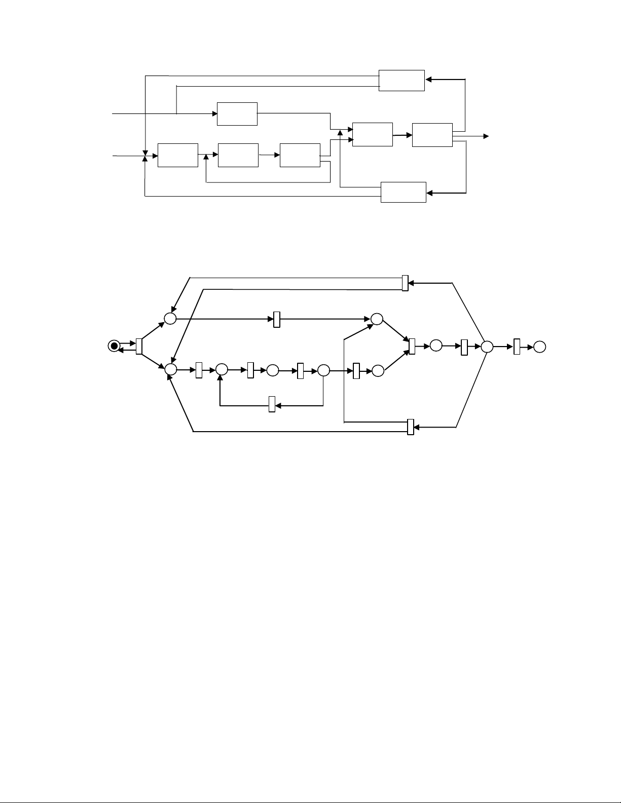
to machines 1 and 2 and two B-parts to machine 3. The flow is illustrated in Fig. 15.6. Disassembler 2 Parts of type 2 Machine 3 Assembler Parts of Inspector 2 t ype 1 Uninstalled Machine 1 Machine 2 Inspector 1 Disassembler 1
Fig. 15.6. A manufacturing system 2 t12 p7 t7 p8 2 t1 2 t8 t9 t 10 2 t2 t3 p1 t4 p5 t5 p9 p 10 p11 p2 p3 p4 p6 t6 t11
Fig. 15.7. Petri net model of the manufacturing system in Fig. 15.6.
Fig. 15.7 shows the Petri net model of this system. The legends of places and transitions in this model are as follows:
p1: Parts ready p2: A-part
p3: A-part after processed by machine 1
p4: B-part after processed by machine 2
p5: Inspection result of inspector 1 p6:
A-part for assembly p7: B-part
p8: B-part for assembly p9:
Assembled product p10: Inspection
result of inspector 2 p11: Final product
t1: One A-part and two B-parts arrive t2:
Machine 1 works on an A-part t3: Machine 2
works on an A-part t4: Inspector 1 examines
an A-part t5: A-part satisfies quality
requirements t6: A-part doesn’t satisfy quality
requirements t7: Machine 3 works on B-part t8: Assembler works
t9: Inspector 2 examines assembled product
t15: Final product is unloaded t11:
Disassembler 1 works t12: Disassembler 2 works
Notice that the two inspectors are modeled by t4 and t9. Their output places, namely p5 and p10, are decision points,
each of which has multiple conflicting outgoing transitions. One the other hand, the transition t9 models a merging (synchronization) action. 15.3 Formal Definition
A Petri net is formally defined as a 5-tuple N = (P, T, I, O, M0), where
(1) P = {p1, p2, , pm} is a finite set of places;
(2) T = {t1, t2, , tn} is a finite set of transitions, P T , and P T = ;
(3) I: T P N is an input function that defines directed arcs from places to transitions, where N is a set of nonnegative integers;
(4) O: T P N is an output function that defines directed arcs from transitions to places; and
(5) M0: P N is the initial marking.
A marking in a Petri net is an assignment of tokens to the places of a Petri net. An arc directed from a place pj to
a transition ti defines pj to be an input place of ti, denoted by I(ti, pj) = 1. An arc directed from a transition ti to a place
pj defines pj to be an output place of ti, denoted by O(ti, pj) = 1. If I(ti, pj) = k (or O(ti, pj) = k), then there exist k directed
(parallel) arcs connecting place pj to transition ti ( or connecting transition ti to place pj).
The formal description of the Petri net in Fig. 15.1 is as follows:
P = {p1, p2, p3, p4, p5};
T = {t1, t2, t3, t4};
I(t1, p1) = 1, I(t1, pi) = 0 for i = 2, 3, 4, 5;
I(t2, p1) = 1, I(t2, pi) = 0 for i = 3, 3, 4, 5;
I(t3, p3) = 2, I(t3, pi) = 0 for i = 1, 2, 4, 5;
O(t1, p2) = 1, O(t1, pi) = 0 for i = 1, 2, 4, 5;
O(t2, p3) = 2, O(t2, p4) = 1, O(t2, pi) = 0 for i = 1,3, 5;
O(t3, p5) = 1, O(t3, pi) = 0 for i = 1, 2, 3, 4;
O(t4, p5) = 1, O(t4, pi) = 0 for i = 1, 2, 3, 4; M0 = (1 0 0 0 0)T.
Mathematically, a transition t is said to be enabled iff M(p)
I(t, p) for all p in P.
For example, the above condition holds for the Petri net of Fig. 15.1 at the initial marking M0, for transitions t1 and t2.
Therefore, t1 and t2 are enabled and can fire. But for t3, because M0(p3) = 0 while I(t3, p3) = 2, the condition does not
hold. Therefore, t3 is not enabled at M0.
The new marking M achieved by firing t at M can be calculated by
M (p) = M(p) I(t, p) + O(t, p) for all p in P.
Consider the Petri net shown in Fig. 15.1 again. Under the initial marking, M0 = (1 0 0 0 0)T, t1 and t2 are
enabled. Firing of t1 results in a new marking, say M1. It follows from the firing rule that M1 = (0 1 0 0 0) T.
The Petri net is dead now because no transitions are enabled at t2. If t2 fires at M0 instead of t1, the new marking, say M2, is M2 = (0 0 2 1 0) T.
At M2, both transitions t3 and t4 are enabled. If t3 fires, the new marking, say M3, is: M3 = (0 0 0 1 1) T.
If t4 fires, the new marking, say M4, is: M4 = (0 0 2 0 1) T.
At M3, t4 can fire, while At M4, t3 can fire. In either case, a new marking, say M5 is reached: M5 = (0 0 0 0 2) T. M5 is a dead marking. p1 t1 t2 t3 p 1 t 1 t 2 t 3 (a) Sequential (b) Conflict 1 p t1 p1 t p 1 2 t2 p2 t3 p3 p 3 (c) Concurrent (d) Synchronization t1 t3 p1 p t 1 1 p2 p3 p2 t2 t4 t2
(e) Mutual exclusive (f) Priority
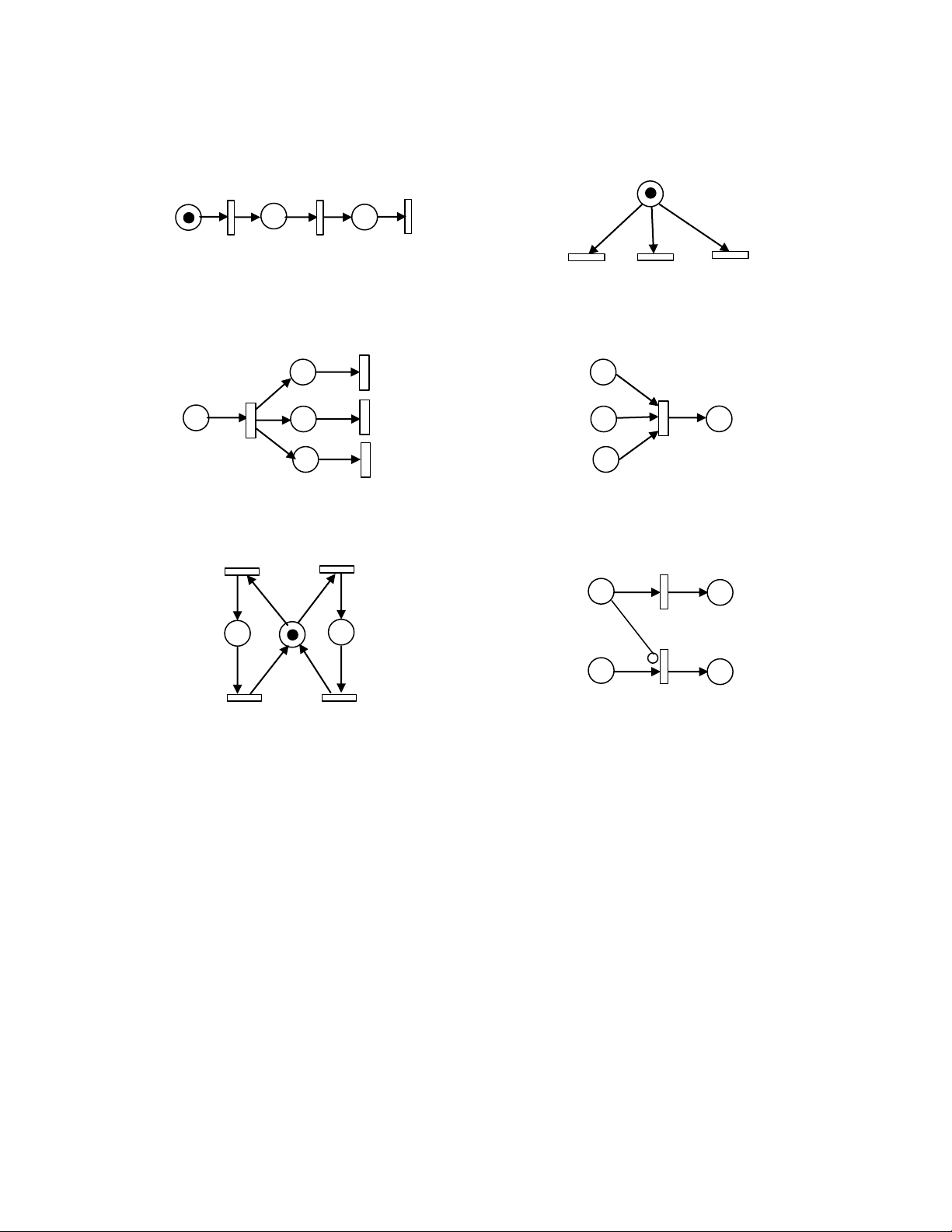
Fig. 15.8. Typical Petri net structures. 15.4 Modeling Power
The typical characteristics exhibited by the activities in a dynamic event-driven system, such as concurrency, decision
making, synchronization and priorities, can be modeled effectively by Petri nets. 1.
Sequential Execution. In Fig. 15.8(a), transition t2 can fire only after the firing of t1 and transition t3 can fire
only after the firing of t2. This imposes the precedence constraint “t3 after t2 and t2 after t1.” Such precedence constraints
are typical of the execution of the parts in a dynamic system. Also, this Petri net construct models the causal
relationship among activities. A practical example is transitions t2, t3 and t4 in Fig. 15.4, which model events “Machine
1 works on an A-part”, “Machine 2 works on an A-part” and “Inspector 1 examines an A-part”, respectively. These
three events occur sequentially in the system. 2.
Conflict. Transitions t1, t2 and t3 are in conflict with each other in Fig. 15.8(b). All are enabled but the firing
of any transition leads to the disabling of the other two transitions. Such a situation will arise, for example, when a
machine has to choose among part types or a part has to choose among several machines. The resulting conflict may
be resolved in a purely non-deterministic way or in a probabilistic way, by assigning appropriate probabilities to the conflicting transitions. 3.
Concurrency. In Fig. 15.8(c), the transitions t1, t2 and t3 are concurrent. Concurrency is an important attribute
of system interactions. In the manufacturing system example of Fig. 15.7, t2 and t7 are concurrent, because after t1 fires,
both p2 and p6 get a token. t2 and t7 model events “Machine 1 works on an A-part” and “Machine 3 works on an B-part”,
respectively, which can happen at the same time. 4.
Synchronization. It is quite normal in a dynamic system that an event requires multiple resources. The
resulting synchronization of resources can be captured by transitions of the type shown in Fig. 15.8(d). Here, t1 is
enabled only when each of p1, p2 and p3 receives a token. The arrival of a token into each of the three places could be
the result of a possibly complex sequence of operations elsewhere in the rest of the Petri net model. Essentially,
transition t1 models the joining operation. 5.
Mutually exclusive. Two processes are mutually exclusive if they cannot be performed at the same time due
to constraints on the usage of shared resources. Fig. 15.8(e) shows this structure. For example, a robot may be shared
by two machines for loading and unloading. Two such structures are parallel mutual exclusion and sequential mutual exclusion. 6.
Priorities. The classical Petri nets discussed so far have no mechanism to represent priorities. Such a
modeling power can be achieved by introducing an inhibitor arc. The inhibitor arc connects an input place to a
transition, and is pictorially represented by an arc terminated with a small circle. The presence of an inhibitor arc
connecting an input place to a transition changes the transition enabling conditions. In the presence of the inhibitor
arc, a transition is regarded as enabled if each input place, connected to the transition by a normal arc (an arc terminated
with an arrow), contains at least the number of tokens equal to the weight of the arc, and no tokens are present on each
input place connected to the transition by the inhibitor arc. The transition firing rule is the same for normally connected
places. The firing, however, does not change the marking in the inhibitor arc connected places. A Petri net with an
inhibitor arc is shown in Fig. 15.8(f). t1 is enabled if p1 contains a token, while t2 is enabled if p2 contains a token and
p1 has no token. This gives priority to t1 over t2: In a marking in which both p1 and p2 have a token, t2 won’t be able to
fire until t1 is fired. 15.5 Petri Net Analysis
We have introduced the modeling power of Petri nets in the previous sections. However, modeling by itself is of little
use. It is necessary to analyze the modeled system. This analysis will hopefully lead to important insights into the
behavior of the modeled system.
There are four common approaches to Petri net analysis: 1) reachability analysis, 2) the matrix-equation approach,
3) invariant analysis, and 4) simulation. The first approach involves the enumeration of all reachable markings, but it
suffers from the state-space explosion issue. The matrix equations technique is powerful but in many cases it is
applicable only to special subclasses of Petri nets or special situations. The invariant analysis determines sets of places
or transitions with special features, as token conservation or cyclical behavior. For complex Petri net models, discrete-
event simulation is an option to check the system properties.
15.5.1 Reachability Analysis
Reachability analysis is conducted through the construction of reachability tree if the net is bounded. Given a Petri net
N, from its initial marking M0, we can obtain as many “new” markings as the number of the enabled transitions. From
each new marking, we can again reach more markings. Repeating the procedure over and over results in a tree
representation of the markings. Nodes represent markings generated from M0 and its successors, and each arc
represents a transition firing, which transforms one marking to another.
The above tree representation, however, will grow infinitely large if the net is unbounded. To keep the tree finite,
we introduce a special symbol , which can be thought of as “infinity”. It has the properties that for each integer n,
> n, + n = and ≥ . Generally speaking, we don’t know if a Petri net is bounded or not before we perform the
reachability analysis. However, we can construct a coverability tree if the net is unbounded or a reachability tree if the
net is bounded according to the following general algorithm:
1. Label the initial marking M0 as the root and tag it “new”.
2. For every new marking M:
2.1 If M is identical to a marking already appeared in the tree, then tag M “old” and go to another new marking.
2.2 If no transitions are enabled at M, tag M “dead-end” and go to another new marking.
2.3 While there exist enabled transitions at M, do the following for each enabled transition t at M:
2.3.1 Obtain the marking M that results from firing t at M.
2.3.2 On the path from the root to M if there exists a marking M such that M (p) M (p) for each place
p and M M , i.e. M is coverable, then replace M (p) by for each p such that M (p) > M (p).
2.3.3 Introduce M as a node, draw an arc with label t from M to M , and tag M “new”.
If appears in a marking, then the net is unbounded and the tree is a coverability tree, otherwise, the net is bounded
and the tree is a reachability tree. Merging the same nodes in a coverability tree (reachability tree) results in a
coverability graph (reachability graph).
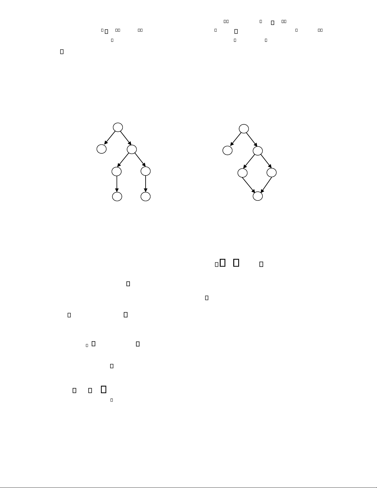
Example 3: Reachability analysis.
Consider the Petri net shown in Fig. 15.1. The analysis in Section 15.3 indicates 5 reachable markings:
M0 = (1 0 0 0 0)T, M1 = (0 1 0 0 0)T, M2 = (0 0 2 1 0)T, M3 = (0 0 0 1 1)T, M4 = (0 0 2 0 1)T, M5 = (0 0 0 0 2)T. The
reachability tree of this Petri net is shown in Fig. 15.9(a), and the reachability graph is shown in Fig. 15.9(b). M root 0 M 0 t t 1 2 t t 1 2 M 1 M M 2 1 t M 2 3 t 4 dead - end t 3 t 4 M 3 M M 4 3 M 4 t 4 t 3 t 4 t 3 M 5 M 5 M 5 dead-end old
Fig. 15.9 (a) Reachability tree. (b) Reachability graph.
16.5.2 Incidence matrix and state equation
For a Petri net with n transitions and m places, the incidence matrix A aij
is an n m matrix of integers and its
entry is given by aij = O(ti, pj) I(ti, pj).
In writing matrix equations, we write a marking Mk as an m 1 column vector. The j-th entry of Mk denotes the
number of tokens in place j immediately after the k-th firing in some firing sequence. The k-th firing or control vector
uk is an n 1 column vector of n 1 0’s and one nonzero entry, a 1 in the i-th position indicating that transition i fires
at the k-th firing. Since the i-th row of the incidence matrix A denotes the change of the marking as the result of firing
transition i, we can write the following state equation for a Petri net:
Mk = Mk 1 ATuk , k = 1, 2,
Suppose that a destination marking Md is reachable from M0 through a firing sequence {u1, u2 …, ud}. Writing the
state equation for k = 1, 2, , d and summing them, we obtain d
Md M0 AT uk k 1 15.5.3 Software tools
For complex Petri net models, simulation is another way to check the system properties. The idea is simple, that is,
using the execution algorithm to run the net. Simulation is an expensive and time-consuming technique. It can show
the presence of undesirable properties but cannot prove the correctness of the model in general case. Despite this, Petri
net simulation is indeed a convenient and straightforward yet effective approach for engineers to validate the desired
properties of a discrete event system. For this reason, many software tools have been developed by Petri net
researchers. A list of Petri net simulation tools along with feature descriptions can be found in the following Petri Nets World website:
http://www.informatik.uni-hamburg.de/TGI/PetriNets/ 15.6 Petri Net Properties
As a mathematical tool, Petri nets possess a number of properties. These properties, when interpreted in the context of
the modeled system, allow system designer to identify the presence or absence of the application domain specific
functional properties of the system under design. Two types of properties can be distinguished, behavioral and
structural ones. The behavioral properties are those which depend on the initial state or marking of a Petri net. The
structural properties, on the other hand, do not depend on the initial marking of a Petri net. They depend on the
topology, or net structure, of a Petri net. In this section, we briefly introduce three behavioral properties: reachability,
safeness, and liveness, and two structural properties: invariants, and siphons and traps. 15.6.1 Reachability
An important issue in designing event-driven systems is whether a system can reach a specific state, or exhibit a
particular functional behavior. In general, the question is whether the system modeled with a Petri net exhibits all
desirable properties as specified in the requirement specification, and no undesirable ones.
In order to find out whether the modeled system can reach a specific state as a result of a required functional
behavior, it is necessary to find such a transition firing sequence that would transform its Petri net model from the
initial marking M0 to the desired marking Mj, where Mj represents the specific state, and the firing sequence represents
the required functional behavior. In general, a marking Mj is said to be reachable from a marking Mi if there exists a
sequence of transitions firings which transforms Mi to Mj. A marking Mj is said to be immediately reachable from Mi
if firing an enabled transition in Mi results in Mj. The set of all markings reachable from marking M is denoted by R(M).
For example, as shown in Fig. 15.9, the Petri net of Fig. 15.1 has five reachable markings, in which M1 and M2
are immediately reachable from the initial marking M0. 15.6.2 Safeness
In a Petri net, places are often used to represent information storage areas in communication and computer systems,
product and tool storage areas in manufacturing systems, etc. It is important to be able to determine whether proposed
control strategies prevent from the overflows of these storage areas. The Petri net property which helps to identify the
existence of overflows in the modeled system is the concept of boundedness.
A place p is said to be k-bounded if the number of tokens in p is always less than or equal to k (k is a nonnegative
integer number) for every marking M reachable from the initial marking M0, i.e., M R(M0). It is safe if it is 1- bounded.
A Petri net N = (P, T, I, O, M0) is k-bounded (safe) if each place in P is k-bounded (safe). It is unbounded if k is
infinitely large. For example, the Petri net of Fig. 15.1 is 2-bounded, but the net of Fig. 15.3 is unbounded, because if
transitions write and send keep firing, the place mail_box will get infinite number of tokens. 15.6.3 Liveness
The concept of liveness is closely related to the deadlock situation, which has been situated extensively in the context
of computer operating systems.
A Petri net modeling a deadlock-free system must be live. This implies that for any reachable marking M, it is
ultimately possible to fire any transition in the net by progressing through some firing sequence. This requirement,
however, might be too strict to represent some real systems or scenarios that exhibit deadlock-free behavior. For
instance, the initialization of a system can be modeled by a transition (or a set of transitions) which fire a finite number
of times. After initialization, the system may exhibit a deadlock-free behavior, although the Petri net representing this
system is no longer live as specified above. For this reason, different levels of liveness are defined. Denote by L(M0)
the set of all possible firing sequences starting from M0.A transition t in a Petri net is said to be:
(1) L0-live (or dead) if there is no firing sequence in L(M0) in which t can fire.
(2) L1-live (potentially firable) if t can be fired at least once in some firing sequence in L(M0).
(3) L2-live if t can be fired at least k times in some firing sequence in L(M0) given any positive integer k.
(4) L3-live if t can be fired infinitely often in some firing sequence in L(M0).
(5) L4-live (or live) if t is L1-live (potentially firable) in every marking in R(M0).
For example, all the three transitions in the net of Fig. 15.1 are L1-live because all of the four transitions can only
fire once. However, all transitions in the net of Fig. 15.4 are L4-live, because they are all L1-live in every reachable marking. 15.6.4 Invariants
In a Petri net, arcs describe the relationships among places and transitions. They are represented by two matrices I and
O. By examining the linear equations based on the execution rule and the matrices, one can find subsets of places over
which the sum of the tokens remains unchanged. One may also find a transition firing sequence brings the marking
back to the same one. The concepts of S-invariant and T-invariant are introduced to reflect these properties.
Mathematically, an S-invariant is an integer solution y of the homogeneous equation
Ay = 0, and a T-invariant is an integer solution x of the homogeneous equation ATx = 0.
The non-zero entries in an S-invariant represent weights associated with the corresponding places so that the weighted
sum of tokens on these places is constant for all markings reachable from an initial marking. These places are said to
be covered by an S-invariant. The non-zero entries in a T-invariant represent the firing counts of the corresponding
transitions which belongs to a firing sequence transforming a marking M0 back to M0. Although a T-invariant states
the transitions comprising the firing sequence transforming a marking M0 back to M0, and the number of times these
transitions appear in this sequence, it doesn’t specify the order of the transition firings.
Invariant findings may help in analysis for some Petri net properties. For example, if each place in a net is covered
by an S-invariant, then it is bounded. However, this approach is of limited use since invariant analysis does not include
all the information of a general Petri net.
The set of places (transitions) corresponding to nonzero entries in an S-invariant y 0 (T-invariant x 0) is called
the support of an invariant and is denoted by | x| (| y| ). A support is said to be minimal if there is no other invariant y1
such that y1(p) y(p) for all p. Given a minimal support of an invariant, there is a unique minimal invariant
corresponding to the minimal support. We call such an invariant a minimal-support invariant. The set of all possible
minimal-support invariants can serve as a generator of invariants. That is, any invariant can be written as a linear
combination of minimal-support invariants.
Example 4:
Figure 15.10 shows a simple manufacturing system with a single machine and a buffer. The capacity of the buffer
is 1. A raw part can enter the buffer only when it is empty, otherwise it is rejected. As soon as the part residing in the
buffer it gets processed, the buffer is released and can accept another coming part. Fault may occur in the machine
when it is processing a part. After being repaired, the machine continues process the uncompleted part. The places and
transitions in this Petri net are as follows:
p1: The buffer (size of two) is empty.
p2: Parts are in buffer. p3: The machine is free.
p4: The machine is processing a part.
p5: The machine is failed. t1: A part
arrives. t2: The machine starts
processing a part. t3: The machine ends
processing a part. t4: The machine fails.
t5: Repair the machine. p 1 p 3 t 3 p t 4 2 t p 1 2 p 5 t t 5 4
Fig. 15.10. A simple manufacturing system with a single machine and a buffer.
We are going to find the S-invariants of the net and use them to see how this simple manufacturing system works.
First we obtain the incidence matrix directly from the model: 1 1 0 0 0 1 1 1 1 0 0 1 1 . A 0 0 0 1 0 0 0 0 1 1 1 0
Then, by solving Ay = 0 we get two minimal-support S-invariants, y1 = (1 1 0 0 0)T and y2 = (0 0 1 1 1)T where | y1| =
{p1, p2} and | y2| = {p3, p4, p4} are corresponding minimal supports. Since the initial marking is M0 = (2 0 1 0 0)T, then M T
0 y1 = 1 and this leads to the fact that M(p1) + M(p2) = 2.
It shows that the buffer is either free or one slot occupied or both slots occupied. Similarly, it results from M T 0 y2 = 1 that
M(p3) + M(p4) + M(p5) = 1.
It shows how the machine spends its time. It is either up and waiting, or up and working, or down.
15.6.5 Siphons and Traps
Let *S and S* denote the sets of input and output transitions of place set S, respectively. Given a PN P = (P, T, I, O,
M0), a subset of places S of P is called a siphon if *S S*. Intuitively, if a transition is going to deposit a token to a
place in a siphon S, the transition must also remove a token from S. On the other hand, a subset of places S of P is
called a trap if S* *S. Intuitively, a trap S represents a set of places in which every transition consuming a token
from S must also deposit a token back into S.
For example, the set S = {w_rest, mail, mail_box} in the Petri net of Fig. 15.3 is a siphon, because *S = {write,
send}, S* = {write, send, receive} and thus *S S*. The set S = {mail_box, r_rest, received} in the same Petri net is
a siphon, because S* = {receive, read}, S* = {send, receive, read} and thus S* *S. 15.7 Colored Petri Nets
In a standard Petri net, tokens are indistinguishable. Because of this, Petri nets have the distinct disadvantage of
producing very large and unstructured specifications for the systems being modeled. To tackle this issue, high-level
Petri nets were developed to allow compact system representation. Colored Petri nets (Jensen 1981) and
Predicate/Transition (Pr/T) nets (Genrich and Lautenbach 1981) are among the most popular high-level Petri nets. We
will introduce colored Petri nets in this section.
Introduced by Kurt Jensen in, a Colored Petri Net (CPN) has its each token attached with a color, indicating the
identity of the token. Moreover, each place and each transition has attached a set of colors. A transition can fire with
respect to each of its colors. By firing a transition, tokens are removed from the input places and added to the output
places in the same way as that in original Petri nets, except that a functional dependency is specified between the color
of the transition firing and the colors of the involved tokens. The color attached to a token may be changed by a
transition firing and it often represents a complex data-value. CPNs lead to compact net models by using of the concept
of colors. This is illustrated by Example 4.
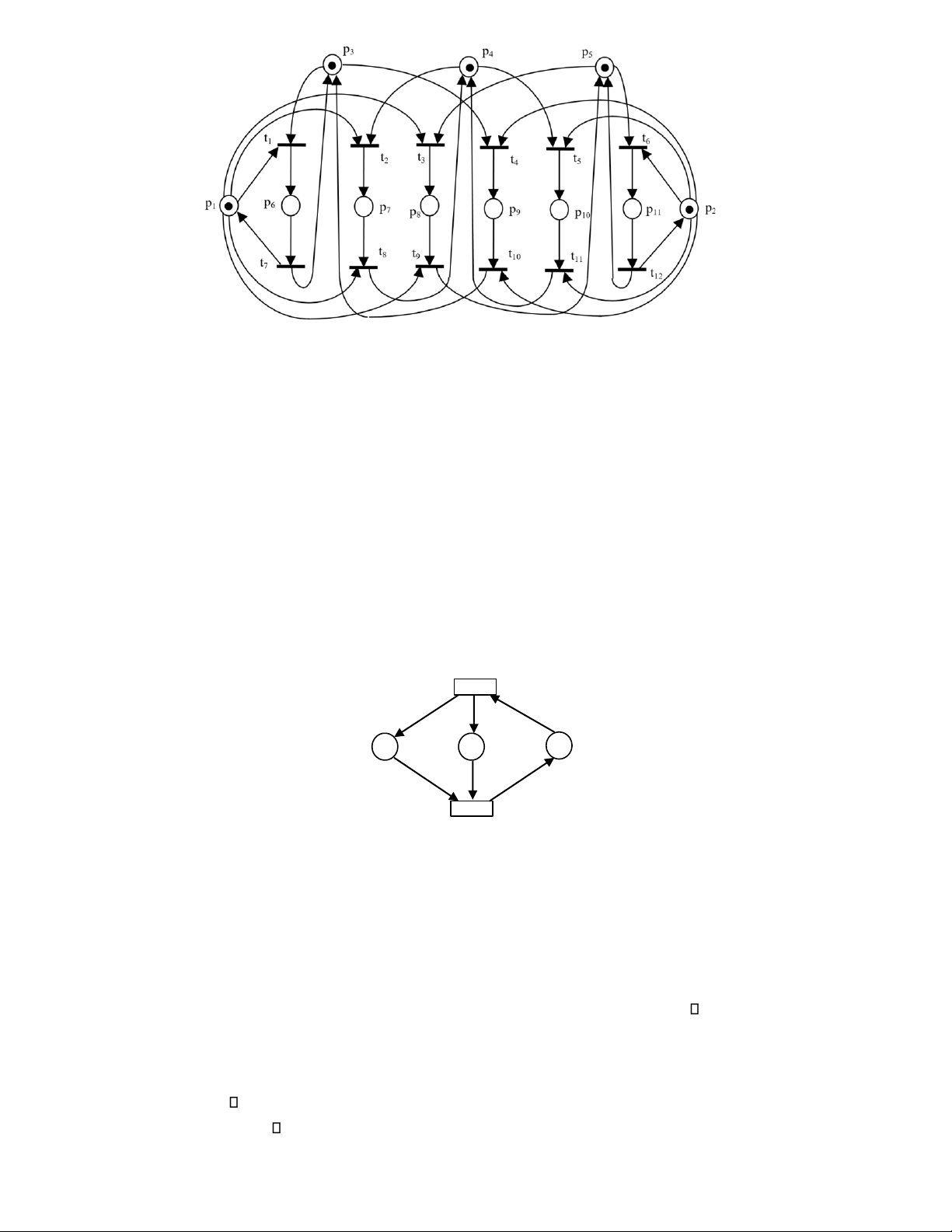
Example 5: A manufacturing system.
Fig. 15.11. Petri net model of a simple manufacturing system.
Consider a simple manufacturing system comprising two machines M1 and M2, which process three different types
of raw parts. Each type of parts goes through one stage of operation, which can be performed on either M1 or M2.
After the completion of processing of a part, the part is unloaded from the system and a fresh part of the same type is
loaded into the system. Fig. 11 shows the (uncolored) Petri net model of the system. The places and transitions in the model are as follows:
p1 (p2): Machine M1 (M2) available
p3 (p4, p5): A raw part of type 1 (type 2, type 3) available p6 (p7, p8):
M1 processing a raw part of type 1 (type 2, type 3) p9 (p10, p11): M2
processing a raw part of type 1 (type 2, type 3) t1 (t2, t3): M1 begins
processing a raw part of type 1 (type 2, type 3) t4 (t5, t6): M2 begins
processing a raw part of type 1 (type 2, type 3) t7 (t8, t9): M1 ends
processing a raw part of type 1 (type 2, type 3) t 15 (t11, t12): M2
ends processing a raw part of type 1 (type 2, type 3) t 1 < M1, M 2> < J1, J2, J 3> p 1 p 3 p 2 t 2
Fig. 15.12. Colored Petri net model of the manufacturing system.
Now let us take a look at the CPN model of this manufacturing system, which is shown in Fig. 12. As we can see,
there are only 3 places and 2 transitions in the CPN model, compared at 11 places and 12 transitions in Fig. 15.11. In
this CPN model, p1 means machines are available (corresponding to places p1 and p2 in Fig. 15.11), p2 means parts
available (corresponding to places p3 − p5 in Fig. 15.11), p3 means processing in progress (corresponding to places p6
− p11 in Fig. 11), t1 means processing starts (corresponding to transitions t1 − t6 in Fig. 11), and t2 means processing ends
(corresponding to transitions t7 − t12 in Fig. 15.11). There are three color sets: SM, SP and SM SP, where SM = {M1,
M2}, SP = {J1, J2, J3}. The color of each node is as follows:
C(p1) = {M1, M2},
C(p2) = {J1, J2, J3},
C(p3) = SM SP,
C(t1) = C(t2) = SM SP.
CPN models can be analyzed through reachability analysis. As for ordinary Petri nets, the basic idea behind
reachability analysis is to construct a reachability graph. Obviously, such a graph may become very large, even for
small CPN’s. However, it can be constructed and analyzed totally automatically, and there exist techniques which
makes it possible to work with condensed occurrence graphs without losing analytic power. These techniques build
upon equivalence classes. Another option to the CPN model analysis is simulation. Readers are referred to (Jensen
1997) for a detailed description of the concepts, analysis methods and practical use of colored Petri nets. 15.8 Timed Petri Nets
The need for including timing variables in the models of various types of dynamic systems is apparent since these
systems are real time in nature. In the real world, almost every event is time related. When a Petri net contains a time
variable, it becomes a Timed Petri Net (Wang 1998). The definition of a timed Petri net consists of three specifications:
• The topological structure, The labeling of the structure, and • Firing rules.
The topological structure of a timed Petri net generally takes the form that is used in a conventional Petri net. The
labeling of a timed Petri net consists of assigning numerical values to one or more of the following things: Transitions, • Places, and
• Arcs connecting the places and transitions.
The firing rules are defined differently depending on the way the Petri net is labeled with time variables. The firing
rules defined for a timed Petri net control the process of moving the tokens around.
The above variations lead to several different types of timed Petri nets. Among them, deterministic time Petri nets
(Ramchandani 1974) and stochastic timed Petri nets (Molloy 1982; Bause and Kritzinger 2002), in which time
variables are associated with transitions, are the two most widely used extended Petri nets.
15.8.1 Deterministic Timed Petri Nets
The introduction of deterministic time labels into Petri nets was first attempted by Ramchandani (Ramchandani 1974).
In his approach, the time labels were placed at each transition, denoting the fact that transitions are often used to
represent actions, and actions take time to complete. The obtained extended Petri nets are called Deterministic Timed
Petri Nets (DTPNs for short). (Ramamoorthy and Ho 1980) used such an extended model to analyze system
performance. The method is applicable to a restricted class of systems called decision-free nets. This class of nets
involves neither decisions nor non-determinism. In structural terms, each place is connected to the input of no more
than one transition, and to the output of no more than one transition.
A deterministic timed transitions Petri net (DTPN) is a 6-tuples (P, T, I, O, M0, ), where (P, T, I, O, M0) is a Petri
net, : T R+ is a function that associates transitions with deterministic time delays.
A transition ti in a DTPN can fire at time if and only if
(1) for any input place p of this transition, there have been the number of tokens equal to the weight of the
directed arc connecting p to ti in the input place continuously for the time interval [
i, ], where i is the
associated firing time of transition ti;
(2) After the transition fires, each of its output places, p, will receive the number of tokens equal to the weight
of the directed arc connecting ti to p at time .
An important application of DTPN is to calculate the cycle time of a Petri net model. For a decision-free Petri net
where every place has exactly one input arc and one output arc, the minimum cycle time (maximum performance) C is given by
Tk :k 1,2,,q} C max{ Nk where Tk
i sum of the execution times of the transitions in circuit k; ti Lk
Nk M(pi )= total number of tokens in the places in circuit k; pi Lk
q = number of circuits in the net.
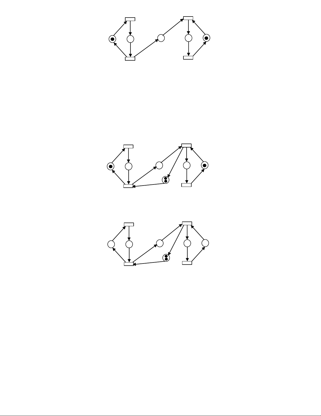
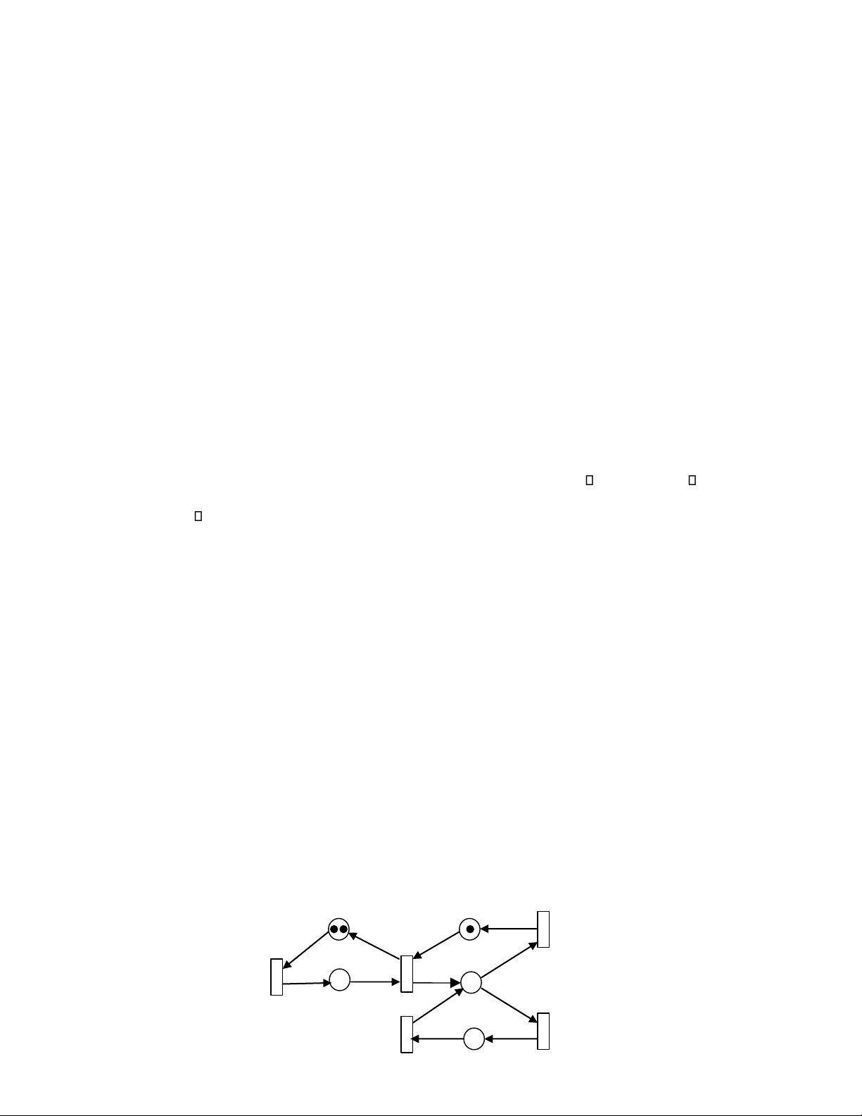
Example 6: A communication protocol.
Consider the communication protocol between two processes, one indicated as the sender, and the other as the
receiver. The sender sends messages to a buffer, while the receiver picks up messages from the buffer. When it gets a
message, the receiver sends an ACK back to the sender. After receiving the ACK from the receiver, the sender begins
processing and sending a new message. Suppose that the sender takes 1 time unit to send a message to the buffer, 1
time unit to receive the ACK, and 3 time units to process a new message. The receiver takes 1 time unit to get the
messages from the buffer, 1 time unit to send back an ACK to the buffer, and 4 time units to process a received message.
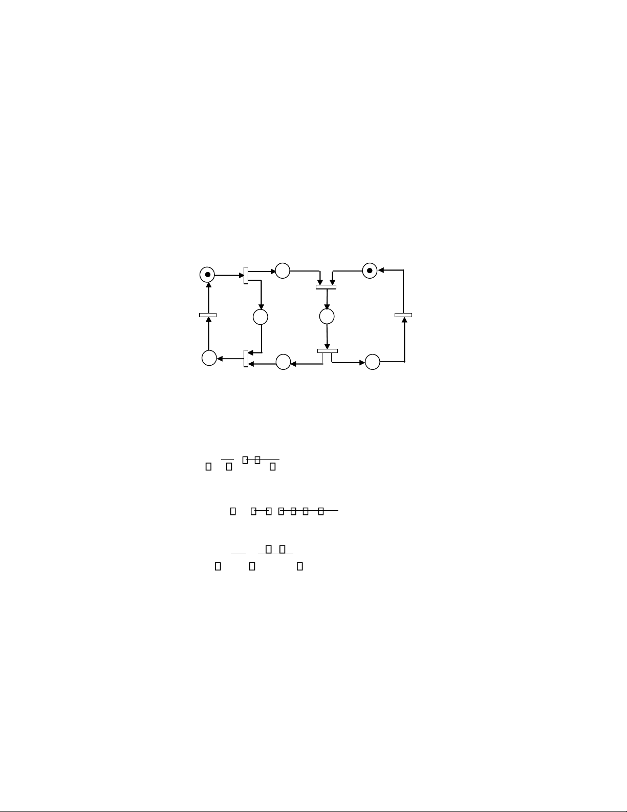
The DTPN model of this protocol is shown in Fig. 15.13. The legends of places and transitions and timing properties
are as follows: p1: The sender ready p2: Message in the buffer p3: The sender waiting for ACK p4: Message received
p5: The receiver ready p6: ACK sent p7: ACK in the buffer p8: ACK received t1: The sender sends a message to the
buffer. Time delay: 1 time unit.
t2: The receiver gets the messages from the buffer. Time delay: 1 time unit.
t3: The receiver sends back an ACK to the buffer. Time delay: 1 time unit.
t4: The receiver processes the message. Time delay: 4 time units. t5: The
sender receivers the ACK. Time delay: 1 time unit.
t6: The sender processes a new message. Time delay: 3 time units. p 2 p 5 p t 1 1 t 2 t 6 p t 4 3 p 4 t 3 p 8 t 5 p 7 p 6
Fig. 15.13. Petri net model of a simple communication protocol.
There are three circuits in the model. The cycle time of each circuit is calculated as follows:
circuit p1t1p3t5p8t6p1 : C1 T1 1 1 3 5, N1 1
circuit p1t1p2t2p4t3p7t5p8t6p1 : C2 T2 1 1 1 1 3 7 , N2 1 T3 1 1 4 6.
circuit p5t2p4t3p6t4p5 : C3 N3 1
After enumerating all circuits in the net, we know the minimum cycle time of the protocol between the two processes is 7 time units.
15.8.2 Stochastic Timed Petri Nets
Stochastic timed Petri nets (STPN’s) are Petri nets in which stochastic firing times are associated with transitions. An
STPN is essentially a high-level model that generates a stochastic process. STPN-based performance evaluation
basically comprises modeling the given system by an STPN and automatically generating the stochastic process that
governs the system behavior. This stochastic process is then analyzed using known techniques. STPN’s are a graphical
model and offer great convenience to a modeler in arriving at a credible, high-level model of a system.
The simplest choice for the individual distributions of transition firing times is negative exponential distribution.
Because of the memoryless property of this distribution, the stochastic process associated with the STPN is a
continuous time homogeneous Markov chain with state space in one to one correspondences to with marking in R(M0),
the set of all reachable markings. The transition rate matrix of the Markov chain can be easily constructed from the
reachability graph given the firing rates of the transitions of the STPN. Exponential timed stochastic Petri nets, often
called Stochastic Petri Nets (SPNs), were independently proposed by Natkin (Natkin 1980) and Molloy (Molloy 1981),
and their capabilities in the performance analysis of real systems have been investigated by many authors.
An SPN is a six-tuple (P, T, I, O, M0, ) in which (P, T, I, O, M0) is a Petri net and : T R is a set of firing rates
whose entry k is the rate of the exponential individual firing time distribution associated with transition tk. Natkin
and Molloy have shown that the marking process of an SPN is a continuous time Markov chain. The state space of the
Markov chain is the reachable set R(M0). Suppose there are s markings in R(M0), and the underlying Markov chain is
ergodic, then the steady state probability distribution = ( 0, 1, …, s) can be obtained by resolving the following linear system: Q = 0
j 1, where j ≥ 0, j = 0, 1, 2, …
j where Q is a transition rate matrix whose elements outside the main diagonal are the rates of the
exponential distributions associated with the transitions from state, while the elements on the main diagonal make
the sum of the elements of each row equal to zero. Denote by E(Mi) the set of all enabled transition at marking Mi,
and Tij the set of enabled transitions at marking Mi whose firings lead the SPN to another marking Mj. Then Q is determined as follows: qi j k , tk Ti j qi qii k . tk E(Mi )
The probability of marking Mi changing to Mj is the same as the probability that one of the transitions in the set
Tij fires before any of the transitions in the set T \ Tij. Since the firing times in an SPN are mutually independent
exponential random variables, it follows that the required probability has the specific value given by
ij = qij / qi.
In the expression for ij deduced above, note that the numerator is the sum of the rates of those enabled transitions in
Mi, the firing of any of which changes the marking from Mi to Mj; whereas the denominator is the sum of the rates of
all the enabled transitions in Mi. Also note that ij = 1 if and only if Tij = E(Mi).
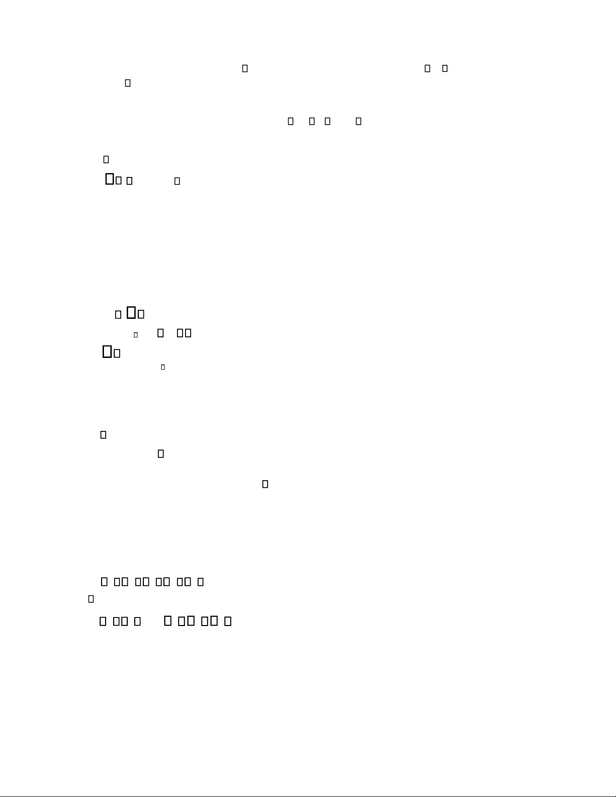
Example 7: A stochastic Petri net.
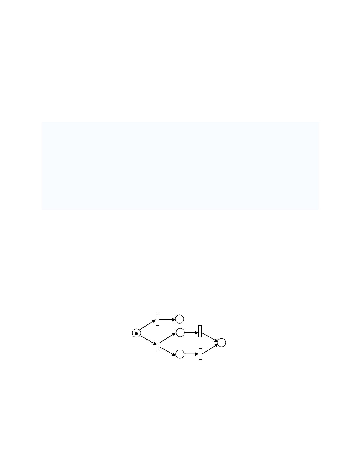
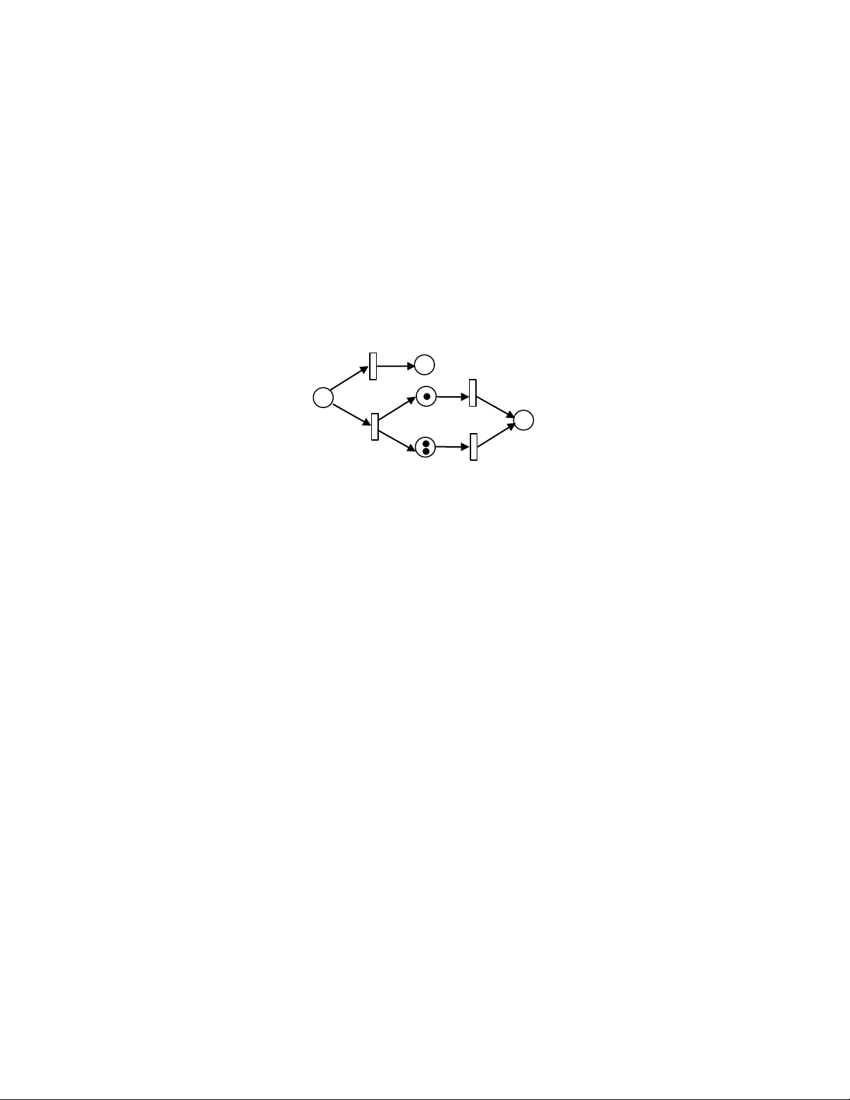
Fig. 15.14 shows a simple SPN model with its reachable markings and its reachable graph. The linear system of steady state probabilities is 0 1 2 3 4 1
Let = (1 1 1 1), then solution to this system is: 0 4 2/7, 1 2 3 1/7. M t 2 t 3 t 1 1 t 4 t 1 M 0 M 4 t 3 t 2 p p 5 M 3 t 3 3 t 4 p 1 p2 t2 p4 M2
Fig. 15.14. (a) SPN model. (b) Reachability graph
The analysis of an SPN model is usually aimed at the computation of more aggregate performance indices than
the probabilities of individual markings. Several kinds of aggregate results can easily be obtained from the steady state
distribution over reachable markings, such as the probability of an event defined through place markings, the average
number of tokens in a place, the frequency of firing a transition, i.e., the average number of times the transition fires
in unit time, and the average delay of a token in traversing a subnet in steady state conditions (Ajmone Marsan 1990). 15.9
Continuous Petri Nets and Hybrid Petri Nets
The Petri nets we have discussed so far are all discrete Petri nets, because transitions fire at certain instants with zero
duration. A continuous Petri net has the same structure as a discrete Petri net. The main difference is that a transition
in a continuous Petri net fires continuously with a flow that may be externally generated by an input signal and may
also depend on the continuous making. A continuous place can hold a nonnegative real number as its content. A
continuous transition fires continuously at the speed of a parameter assigned at the continuous transition. Continuous
Petri nets are suitable for modeling systems in which continuous or batch material flows go through a number of stages
of processing (Pettersson and Lennartson, 1995).
Hybrid Petri nets (Alla and David, 1998) are an extension to traditional Petri nets with introduction of continuous
places and continuous transitions, or a mixture of discrete Petri nets and continuous Petri nets. Therefore, a hybrid
Petri net has a discrete part and a continuous part. The discrete part models the logic functioning of a system and the
continuous part models a system with continuous flows. 15.10 Concluding Remarks
Petri nets have been proven to be a powerful modeling tool for various types of dynamic event-driven systems. Since
Petri nets were introduced in 1962, numerous research papers have been published. The research has been conducted
on many branches, with each branch exploring a promising application aspect of this formalism. Given the rich
research results from the Petri net society, it is hard to cover all of them in such a short book chapter. Therefore, this
chapter only aims at briefly introducing the most basic concepts, theory and applications of ordinary Petri nets and a
few of most popular extended Petri nets. References
van der Aalst, Wil, and Kees van Hee. 2000. Workflow Management: Models, Methods, and Systems. Massachusetts: MIT Press.
Alla, H, David, R. 1998. Continuous and hybrid Petri nets. J Circuits Syst Comput, 8, 159–88.
Ajmone Marsan, M. 1990. Stochastic Petri nets: an elementary introduction. Advances in Petri Nets, LNCS 424.
Ajmone Marsan, M., M. G. Balbo and G. Conte. 1986. Performance Models of Multiprocessor Systems, Massachusetts: The MIT Press.
Andreadakis, S.K., and A.H. Levis. 1988. Synthesis of distributed command and control for the outer air battle.
Proceedings of the 1988 Symposium on C² Research. SAIC, McLean, VA.
Bause, F., and P. Kritzinger. 2002. Stochastic Petri Nets -- An Introduction to the Theory. Germany: Vieweg Verlag.
Desrochers, A., and R. Ai-Jaar. 1995. Applications of Petri Nets in Manufacturing Systems: Modeling, Control and
Performance Analysis. IEEE Press.
Genrich, J.H., and K. Lautenbach, 1981. System modeling with high-level Petri nets. Theoretical Computer Science 13: 109-136.
Haas, P. Stochastic Petri Nets: Modelling, Stability, Simulation. 2002. New York: Springer-Verlag.
Jensen, K. 1981. Colored Petri nets and the invariant-method, Theoretical Computer Science 14: 317-336.
Jensen, K., 1997. Coloured Petri Nets. Basic Concepts, Analysis Methods and Practical Use (3 volumes). London: Springer-Verlag.
van Landeghem, Rik and Carmen-Veronica Bobeanu. 2002. Formal modeling of supply chain: an incremental
approach using Petri nets. 14th European Simulations Symposium and Exhibition Dresden, Germany.
Kitakaze, H., Matsuno, H. and Ikeda N. (2005). Prediction of debacle points for robustness of biological pathways by
using recurrent neural networks, Genome Informatics, 16(1), 192-202.
Lin, C., L. Tian and Yaya Wei. 2002. Performance equivalent analysis of workflow systems, Journal of Software 13(8): 1472-1480.
Lindemann, C. 1998. Performance Modelling with Deterministic and Stochastic Petri Nets. John Wiley and Sons.
Mandrioli, D., A. Morzenti, M. Pezze, P. Pietro S. and S. Silva. 1996. A Petri net and logic approach to the specification
and verification of real time systems. In: Formal Methods for Real Time Computing (C. Heitmeyer and D.
Mandrioli eds), John Wiley & Sons Ltd.
Merlin, P., and D. Farber. 1976. Recoverability of communication protocols - implication of a theoretical study. IEEE
Transactions on Communications 1036-1543.
Molloy, M. 1981. On the Integration of Delay and Throughput Measures in Distributed Processing Models. Ph.D.
Thesis, UCLA, Los Angeles, CA.
Molloy, M. 1982. Performance analysis using stochastic Petri nets. IEEE Transactions on Computers 31(9): 913-917.
Murata, T. 1989. Petri nets: properties, analysis and applications. Proceedings of the IEEE 77(4): 541-580.
Natkin, S. 1980. Les Reseaux de Petri Stochastiques et Leur Application a I’evaluation des Systemes
Informatiques. These de Docteur Ingegneur, Cnam, Paris, France.
Peterson, J. L. 1981. Petri Net Theory and the Modeling of Systems. N.J.: Prentice-Hall.
Petri, C.A. 1962. Kommunikation mit Automaten. English Translation, 1966: Communication with Automata,
Technical Report RADC-TR-65-377, Rome Air Dev. Center, New York.
Pettersson, S. and Lennartson, B. 1995. Hybrid Modelling focused on Hybrid Petri Nets, 2nd European Workshop on
Real-time and Hybrid systems, 303—309.
Ramchandani, C. 1974. Analysis of Asynchronous Concurrent Systems by Petri Nets. Project MAC, TR-120, M.I.T., Cambridge, MA.
Ramamoorthy, C., and G. Ho. 1980. Performance evaluation of asynchronous concurrent systems using Petri nets.
IEEE Transaction on Software Engineering 6(5): 440-449.
Tsai, J., S. Yang, and Y. Chang. 1995. Timing constraint Petri nets and their application to schedulability analysis of
real-time system specifications. IEEE Transactions on Software Engineering 21(1): 32-49.
Wang, J. 1998. Timed Petri Nets, Theory and Application. Boston: Kluwer Academic Publishers.
Wang, J. 2006. Charging information collection modeling and analysis of GPRS networks. IEEE Transactions on
Systems, Man and Cybernetics, Part C 36(6).
Venkatesh, K., M. C. Zhou, and R. Caudill. 1994. Comparing ladder logic diagrams and Petri nets for sequence
controller design through a discrete manufacturing system. IEEE Trans. on Industrial Electronics 41(6): 611-619.
Zhou, M. C., and F. DiCesare. 1989. Adaptive design of Petri net controllers for error recovery in automated
manufacturing systems. IEEE Trans. on Systems, Man, and Cybernetics 19(5): 963-973. View publication stats
Tài liệu liên quan:
-

Báo cáo cuối kỳ môn hệ thống mạng máy tính và CIM
15 8 -

Thành phần chính của hệ thống sản xuất FMS môn FMS & CIM | Trường Đại học Bách Khoa Hà Nội
84 42 -

Bài tập lớn Thiết kế hệ thống chiết rót tự động & dán nhãn chai môn FMS & CIM | Trường Đại học Bách Khoa Hà Nội
110 55 -

Chương 1: Hệ thống sản xuất linh hoạt môn FMS & CIM | Trường Đại học Bách Khoa Hà Nội
95 48 -

Chương 7: Kiểm soát số máy tính và hệ thống NC bằng Tiếng Việt môn FMS & CIM | Trường Đại học Bách Khoa Hà Nội
96 48