Total Factor Productivity Growth of Vietnamese Enterprises | Microeconomics | Trường Đại học Quốc tế, Đại học Quốc gia Thành phố Hồ Chí Minh
Abstract: Total factor productivity growth (TFPG) is an important indicator evaluating the enterprise development model. The aim of this study is to consider the imbalance between TFPG and enterprises growth patterns of sectors and regions in Vietnam. The results of panel data analysis in 2005–2018 show that the growth of Vietnamese enterprises is mainly due to increased capital, especially in the non-state. Tài liệu được sưu tầm và soạn thảo dưới dạng file PDF để gửi tới các bạn cùng tham khảo, ôn tập đầy đủ kiến thức, chuẩn bị cho các buổi học thật tốt. Mời bạn đọc đón xem!
Môn: Microeconomics 613 tài liệu
Trường: Trường Đại học Quốc tế, Đại học Quốc gia Thành phố Hồ Chí Minh 1.9 K tài liệu
Tác giả:


Preview text:
economies Article
Total Factor Productivity Growth of Vietnamese Enterprises by
Sector and Region: Evidence from Panel Data Analysis Hai Quang Nguyen 1,2 1
Faculty of Business Administration, University of Economics and Law, Ho Chi Minh City 71309, Vietnam; nhquang@uel.edu.vn 2
Vietnam National University, Ho Chi Minh City 71309, Vietnam
Abstract: Total factor productivity growth (TFPG) is an important indicator evaluating the enterprise
development model. The aim of this study is to consider the imbalance between TFPG and enterprises
growth patterns of sectors and regions in Vietnam. The results of panel data analysis in 2005–2018
show that the growth of Vietnamese enterprises is mainly due to increased capital, especially in the
non-state enterprise sector and in the Red River Delta. Total factor productivity (TFP) was found to
be present in the non-state and inward foreign investment sectors during the five years 2014–2018. By
comparison, the state-owned enterprise sector fell sharply during the same period. Strong upward
increases in TFP were notable in the Northern Midlands and Mountain areas, the Mekong River
Delta, and the Southeast, while there was a marked downward trend in the Central Highlands and
the Red River Delta, especially marked in the Central Highlands. Thus, the results from this study
are a basis to suggest an appropriate policy mix that helps to improve the performance of enterprises
in different sectors and regions of Vietnam.
Keywords: total factor productivity growth; enterprise sectors; enterprises in regions; panel data anal- ysis
Citation: Nguyen, Hai Quang. 2021.
Total Factor Productivity Growth of
Vietnamese Enterprises by Sector and
Region: Evidence from Panel Data 1. Introduction
Analysis. Economies 9: 109. https://
TFPG reflects the change or development trend of intangible factors such as technology
doi.org/10.3390/economies9030109
innovation, production rationalization, management improvements, upskilling of the labor
force, etc. Moreover, TFPG reflects efficiency in the use of all factors and constitutes an Academic Editor: Michele Meoli
important source of sustained long-term growth (Tan and Virabhak 1998). As a result of
its importance, there have been many studies measuring and evaluating TFPG in various Received: 31 May 2021
countries: for example, in East Asia by Felipe (1999); in the Singapore service industry by Accepted: 3 August 2021
Tan and Virabhak (1998), Mahadevan (2002), Kong and Tongzon (2006); the measurement of Published: 10 August 2021
TFPG in agriculture by Coelli and Rao (2005), Avila and Evenson (2010); technical efficiency,
technological change and TFPG in Chinese state-owned enterprises by Kong et al. (1999);
Publisher’s Note: MDPI stays neutral
the Wu (2011) study of TFPG in China; TFP in manufacturing and the services sector of
with regard to jurisdictional claims in
post transition economies in Eastern Europe by Botri´c et al. (2017), etc. These studies have
published maps and institutional affil- iations.
enriched the theory and measurement methods of TFPG and TFP in different industries, fields, and contexts.
Vietnam is located in Southeast Asia and is a developing country. TFP, therefore, plays
a key development role in narrowing the economic gap with other countries. Consequently,
enterprises have a particularly important role to play in the economy, as the main driver
Copyright: © 2021 by the author.
of Gross Domestic Product (GDP) and source of employment. According to the General
Licensee MDPI, Basel, Switzerland.
Statistics Office of Vietnam (2020), as of 31 December 2018, Vietnam had 610,000 active
This article is an open access article distributed under the terms and
enterprises reporting production and business statistics (accounting for 80.5% of the total
conditions of the Creative Commons
number of active enterprises) and employing around 14.82 million people. As a result,
Attribution (CC BY) license (https://
enterprises contribute the most to the development of the economy. According to the
creativecommons.org/licenses/by/
GSO of Vietnam, they account for more than 60% of the country’s GDP. However, the 4.0/).
effectiveness of enterprises across sectors and regions is patchy.
Economies 2021, 9, 109. https://doi.org/10.3390/economies9030109
https://www.mdpi.com/journal/economies Economies 2021, 9, 109 2 of 17
There are many reasons behind this, such as advantages specific to individual indus-
tries, regions, businesses, and each enterprise’s growth model. Hence, the study of TFPG of
enterprises across sectors and regions in Vietnam is an issue of practical significance. The
study findings provide useful insights into the repercussions of unbalanced development
between sectors and regions. Furthermore, the study can serve as the basis for developing
an appropriate policy mix geared towards improving the performance of enterprises in the
different sectors and regions of Vietnam.
Previous TFP and TFPG studies in Vietnam have addressed various fields and have
been diverse in their scope. These include measuring TFP in agriculture (Bao 2014;
Giang et al. 2019); TFPG in the coal industry (Phuong 2018); TFP in air transport (Quang
2017); TFPG among modes of transport (Quang 2019); TFP in the food industry (Long
2020), TFP in the manufacturing sectors (Huong 2017; Thanh et al. 2020); TPF for foreign
direct investment enterprises (Hien et al. 2019) and state ownership (Le et al. 2021). In
addition, there are a number of studies examining factors affecting TPF, such as: the impact
of the investment climate on TFP in the agricultural sector (Trung and Cuong 2010); the
impact of investment climate on the TFP of manufacturing firms (Giang et al. 2018); the
impact of innovation on the TFP of small and medium-sized enterprises (Hue et al. 2019);
the determinants of TFP in manufacturing industry (Oanh 2019).
These studies are mainly focused on specific industries or specific ownership sec-
tors. The methods used include both the parametric approach (Trung and Cuong 2010;
Quang 2017 ; Giang et al. 2018, 2019; Quang 2019; Oanh 2019; Le et al. 2021) and the non-
parametric approach (Coelli and Rao 2005; Kong and Tongzon 2006; Wu 2011; Bao 2014;
Phuong 2018). In addition, some recent studies also utilized a semi-parametric approach
(Huong 2017 ; Thanh and Van 2020). Most of the parametric and non-parametric approaches
use the Ordinary Least Square (OLS) regression technique to estimate the parameters for
the TFPG calculation or are based on OLS such as robust regression(Bao 2014), Fixed Effect
Models (FEM), and the Random Effects Model (REM) for panel data (Giang et al. 2019;
Le et al. 2021). The semi-parametric approach uses the estimation technique of Olley and
Pakes (1996) (Giang et al. 2018) or the procedure of Ackerberg et al. (2006) (Thanh and Van
2020). These approaches are discussed in Section 2.
While some publications have carried valuable coverage of TFP and TFPG in Viet-
nam, knowledge gaps remain for two main reasons. Firstly, meaningful insights into
the repercussions of unbalanced development can only be obtained by comparing TFPG
among enterprise sectors and enterprises in different regions. However, the author found
no research results relating to this issue; only studies focused on an industry, a specific
locality, or a type of ownership as outlined above. These will form the basis of business
development policies that align with the need for development orientation and enterprise
performance improvement in Vietnam’s various sectors and regions.
Secondly, although the parameters were estimated by different methods, such as OLS,
FEM, REM, robust regression, semi-parametric estimation procedure of Olley and Pakes or
Ackerberg et al., there are other appropriate methods for each data type that needs to be
considered. For example, if the series is not stationary but cointegrated, the cointegration
regression would be appropriate to prevent spurious regression. The above outlines the
motivations behind this study of enterprise TFPG among sectors and regions of Vietnam.
The objective of this paper is to verify the unbalanced development of TFPG and the growth
model of enterprises in the sectors and regions of Vietnam.
The key empirical contribution of this paper will be in detailing the different roles of
TFP, capital, and labor on the growth model of enterprises operating across various sectors
and regions in Vietnam with an updated sample to 2018. To the best of the author’s
knowledge, this is the first attempt to provide useful insights into the repercussions
of unbalanced TFP developments between sectors and regions in Vietnam based on a
consistent data set and methodology.
After the introduction section, the structure of the study includes four further sections:
Section 2 presents a literature review; Section 3 presents the research methodology and Economies 2021, 9, 109 3 of 17
data; Section 4 presents the study results and discussion; and finally, conclusions and
implications from the study results are presented in Section 5. 2. Literature Review
According to Mahadevan (2003), since the early 1940s, the concept of TFPG and
what it measures has been hotly debated, leading to various definitions. Fundamentally,
though, TFPG is determined by the growth rate of the output minus the growth rate of
the input (Mahadevan 2003 ; Felipe and McCombie 2004). Consequently, researchers have
synthesized and proposed two main approaches to measure the TFPG, such as the frontier
approach and the non-frontier approach (Mahadevan 2003; Kong and Tongzon 2006). Each
approach has a method of parameter estimation and non-parametric estimation. Table 1
below summarizes the differences between these two approaches.
Table 1. Different approaches to measuring TFPG.
Frontier Approach: Assumes Technical Inefficiency
Non-Frontier Approach: Assumes Technical Efficiency Parametric Non-parametric Parametric Non-parametric estimation estimation estimation estimation Stochastic frontier Deterministic Average response function Neutral shifting
Data Envelopment Analysis (DEA) Cobb–Douglas production Translog divisia index Non-neutral shifting Stochastic DEA Cobb–Douglas translog Bayesian approach
Source: Kong and Tongzon (2006).
According to Mahadevan (2003), most studies have used the non-frontier approach for
calculating TFP growth. The frontier approach was initiated by Farrell (1957), but it was not
until the late 1970s that the approach was formalized and used for empirical investigation.
The important difference between the frontier and non-frontier approaches lies in the
definition of “frontier”. A frontier refers to a bounding function or, more appropriately, a
set of best obtainable positions. The frontier approach then determines the role of technical
efficiency in a company’s overall performance, while the non-frontier approach assumes
that companies are technically efficient.
However, what the frontier and non-frontier approaches have in common is that
both can be estimated using the parametric or non-parametric approach. The parametric
technique is an econometric estimation of a specific model since it is based on the statistical
properties of the error terms, it allows for statistical testing and hence validation of the
chosen model. The choice of the functional form is crucial to model the data as different
model specifications can give rise to different results.
In the frontier approach, non-parametric techniques by Data Envelopment Analysis
(DEA) are often applied by researchers (Coelli and Rao 2005; Kong and Tongzon 2006;
Wu 2011; Bao 2014; Phuong 2018; Hien et al. 2019). For the non-frontier approach, the
parameter technique, which is estimated by adapting production functions is also com-
monly applied. There are two common ways to obtain TFP based on firm-level production
functions: Cobb–Douglas production functional form, and a translog production function.
It is argued that both approaches have good mathematical properties. However, according
to Giang et al. (2018), the elasticity of the production to the inputs in the Cobb–Douglas
function allows for easier interpretation than the trans logarithmic production. To be more
specific, the translog technique generally suffers from a collinearity problem among the
regressors (Kinda et al. 2011).
When measuring TFP for firms across broad industries or sectors, a simple production
function consisting of two inputs, capital and labor, and an output factor of value-added,
is often used because these are factors that most generally reflect inputs and outputs
(Tan and Virabhak 1998; Felipe 1999; Giang et al. 2018, 2019; Oanh 2019; Thanh and Van
2020; Oanh 2019). When measured within specific industries or firms, inputs can be Economies 2021, 9, 109 4 of 17
extended beyond capital and labor (Bao 2014; Thanh et al. 2020; Le et al. 2021), or outputs
can be measured by the number of products (Quang 2019).
To overcome the problem of endogeneity between inputs and unobserved productivity,
Olley and Pakes (1996) proposed a semi-parametric approach which was later extended by
Levinsohn and Petrin (2003) and Wooldridge (2009). The robustness to measurement errors
is also an advantage of the semi-parametric method (Van Biesebroeck 2007). This approach
is often used to estimate unobserved productivity at the firm level and has been applied to
the measurement of manufacturing firms in Vietnam (Huong 2017; Thanh and Van 2020).
Although there are many different approaches, they can be summarized into three main methods: (1)
The non-parametric approach using DEA; (2)
The parameter approach using the production function (Cobb–Douglas production
and the transformed production function); (3)
The semi-parametric approach estimating Cobb–Douglas production functional form
specified by the methodology of Levinsohn and Petrin (2003).
Non-parametric approaches have the benefit of not assuming a specific functional
form/shape for the frontier. However, they do not provide a general relationship (equation)
regarding the outputs and inputs to enter, as do parametric or semi-parametric approaches.
The frequent techniques to estimate the production function include OLS estimation, the
Olley and Pakes method, and the Levinsohn and Petrin approach.
3. Research Methodology and Data
3.1. Specification Research Model
As it was appropriate to the data source being collected, this study used the parameter
approach and Cobb–Douglas production function estimation to determine TFPG because
it provides an equational relationship regarding outputs and inputs, as discussed above.
The elasticity of the inputs in the Cobb–Douglas function allows for easier interpretation
than the production translog function and is still in common use (Giang et al. 2018, 2019;
Oanh 2019; Thanh and Van 2020; Thanh et al. 2020; Le et al. 2021). As this study uses
estimates for enterprise sectors and enterprise in regions, the enterprises examined do not
belong to a specific industry, and the most common factors that reflect inputs are capital
and labor. Hence, a Cobb–Douglas production function with two inputs is used in this
study, as has been the case with other recent studies (Giang et al. 2018, 2019; Oanh 2019;
Thanh and Van 2020). The simple Cobb–Douglas production function follows Equation (1). Q = AKαLβ (1) where: Q: Amount of output A: TFP K: Amount of capital L: Labor quantity
α and β: The coefficients of the contribution of capital and labor, respectively.
When calculated, TFPG is shown as the percentage increase of output after subtracting
the contribution of the capital increase and increased labor. From Equation (1), the formula
for calculating TFP growth rate has been widely applied by many researchers and takes
the form of Equation (2) (Felipe 1999; Huong 2017; Oanh 2019; Quang 2019; Thanh and Van 2020). GTFP = GQ − (αGK + βGL) (2) where: GTFP: TFPG GQ: Growth rate of output GK: Growth rate of capital Economies 2021, 9, 109 5 of 17 GL: Growth rate of labor
With α + β = 1.α GK and β GL are the contributions of increase in GQ due to capital
increase and increase in labor, respectively.
Because of α + β = 1 (β = 1 − α ), to facilitate the estimation of the parameters,
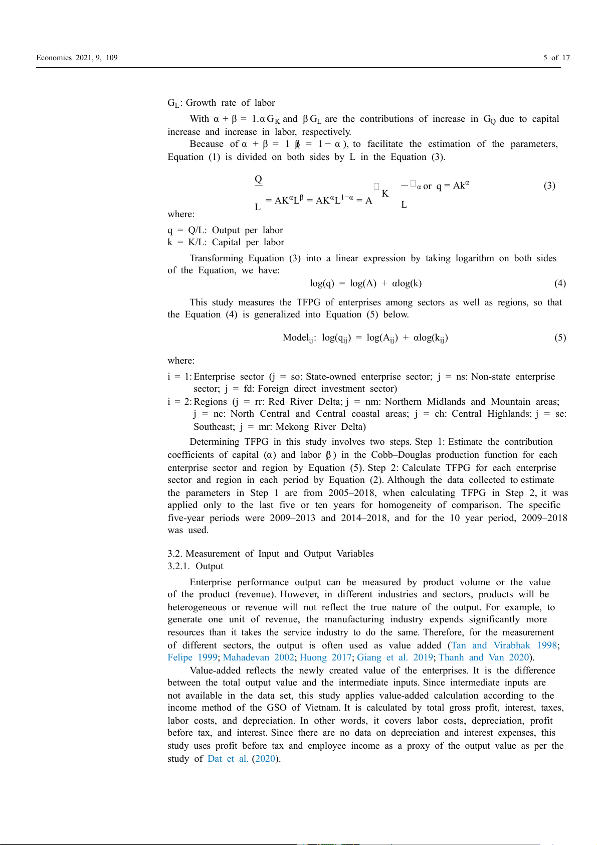
Equation (1) is divided on both sides by L in the Equation (3). Q α α or q = Ak (3) K = AKαLβ = AKαL1−α = A L L where: q = Q/L: Output per labor k = K/L: Capital per labor
Transforming Equation (3) into a linear expression by taking logarithm on both sides of the Equation, we have: log(q) = log(A) + αlog(k) (4)
This study measures the TFPG of enterprises among sectors as well as regions, so that
the Equation (4) is generalized into Equation (5) below.
Modelij: log(qij) = log(Aij) + αlog(kij) (5) where:
i = 1: Enterprise sector (j = so: State-owned enterprise sector; j = ns: Non-state enterprise
sector; j = fd: Foreign direct investment sector)
i = 2: Regions (j = rr: Red River Delta; j = nm: Northern Midlands and Mountain areas;
j = nc: North Central and Central coastal areas; j = ch: Central Highlands; j = se:
Southeast; j = mr: Mekong River Delta)
Determining TFPG in this study involves two steps. Step 1: Estimate the contribution
coefficients of capital (α) and labor (β ) in the Cobb–Douglas production function for each
enterprise sector and region by Equation (5). Step 2: Calculate TFPG for each enterprise
sector and region in each period by Equation (2). Although the data collected to estimate
the parameters in Step 1 are from 2005–2018, when calculating TFPG in Step 2, it was
applied only to the last five or ten years for homogeneity of comparison. The specific
five-year periods were 2009–2013 and 2014–2018, and for the 10 year period, 2009–2018 was used.
3.2. Measurement of Input and Output Variables 3.2.1. Output
Enterprise performance output can be measured by product volume or the value
of the product (revenue). However, in different industries and sectors, products will be
heterogeneous or revenue will not reflect the true nature of the output. For example, to
generate one unit of revenue, the manufacturing industry expends significantly more
resources than it takes the service industry to do the same. Therefore, for the measurement
of different sectors, the output is often used as value added (Tan and Virabhak 1998;
Felipe 1999; Mahadevan 2002; Huong 2017; Giang et al. 2019; Thanh and Van 2020).
Value-added reflects the newly created value of the enterprises. It is the difference
between the total output value and the intermediate inputs. Since intermediate inputs are
not available in the data set, this study applies value-added calculation according to the
income method of the GSO of Vietnam. It is calculated by total gross profit, interest, taxes,
labor costs, and depreciation. In other words, it covers labor costs, depreciation, profit
before tax, and interest. Since there are no data on depreciation and interest expenses, this
study uses profit before tax and employee income as a proxy of the output value as per the study of Dat et al. (2020). Economies 2021, 9, 109 6 of 17
3.2.2. Input Variable: The Volume of Capital
The data commonly used to represent capital are the total assets/ capital sources or
fixed assets. In addition, depending on the availability of data, stock capital is also used
for representation (See and Li 2015; See and Rashid 2016). Based on enterprise survey
data from the GSO of Vietnam, this study used the total annual capital of the enterprise to
represent the amount of capital. Therefore, it is the average of capital at the beginning and the end of the financial year.
3.2.3. Input Variable: The Amount of Labor
The data representing the amount of labor commonly used are the average number of
employees in the financial year (See and Li 2015; See and Rashid 2016;Giang et al. 2019;
Quang 2019) or labor costs (Tan and Virabhak 1998). Based on enterprise survey data
from the GSO of Vietnam, this study used the average number of employees per year to
represent the volume of labor. It is the average number of employees at the beginning and
the end of the year or the average number of employees at the end of two adjacent financial
years as in Equation (6) below. This average method has been implemented in research by
Vasigh and Fleming (2005) or Quang (2019).
Labor at the end of year t − 1 + Labor at the end of year t The average labor in year t = (6) 2 3.3. Research Data
Data from the GSO of Vietnam’s annual report (namely, the “Enterprise, Cooperative
and Non-farm individual business establishment” section) were used by this study to
collate annual data on average capital within the year, the number of employees at the end
of the year, profit before tax, and the income of employees.
The years collected are 2005 and the years 2008–2018. These years were selected as
these are the only years for which the GSO of Vietnam has a full range of official data. The
statistical data relates to all active enterprises as of 31 December of each year. Due to a
change in the division of the state-owned enterprise sector, the data for central enterprises
and local enterprises were collected for 2005 and 2008–2015. Meanwhile, the data for
enterprises with 100% state capital and enterprises where the state holds more than 50% of
charter capital were collected for the year 2010 and during 2013–2018. The annual number
of employees was collected a year ago to calculate the average number of employees. To
ensure the study’s data stability, enterprises with negative or very modest gross profit
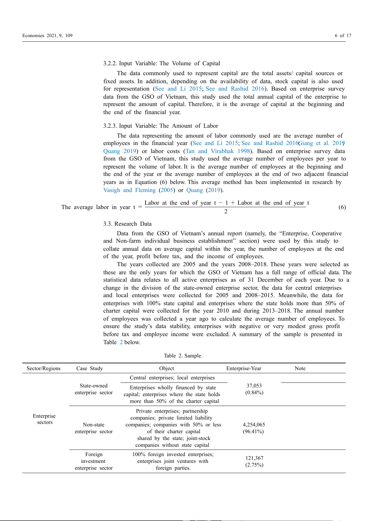
before tax and employee income were excluded. A summary of the sample is presented in Table 2 below. Table 2. Sample. Sector/Regions Case Study Object Enterprise-Year Note
Central enterprises; local enterprises State-owned 37,053
Enterprises wholly financed by state enterprise sector (0.84%)
capital; enterprises where the state holds
more than 50% of the charter capital
Private enterprises; partnership Enterprise
companies; private limited liability sectors Non-state
companies; companies with 50% or less 4,254,065 enterprise sector of their charter capital (96.41%)
shared by the state; joint-stock
companies without state capital Foreign
100% foreign invested enterprises; 121,367 investment
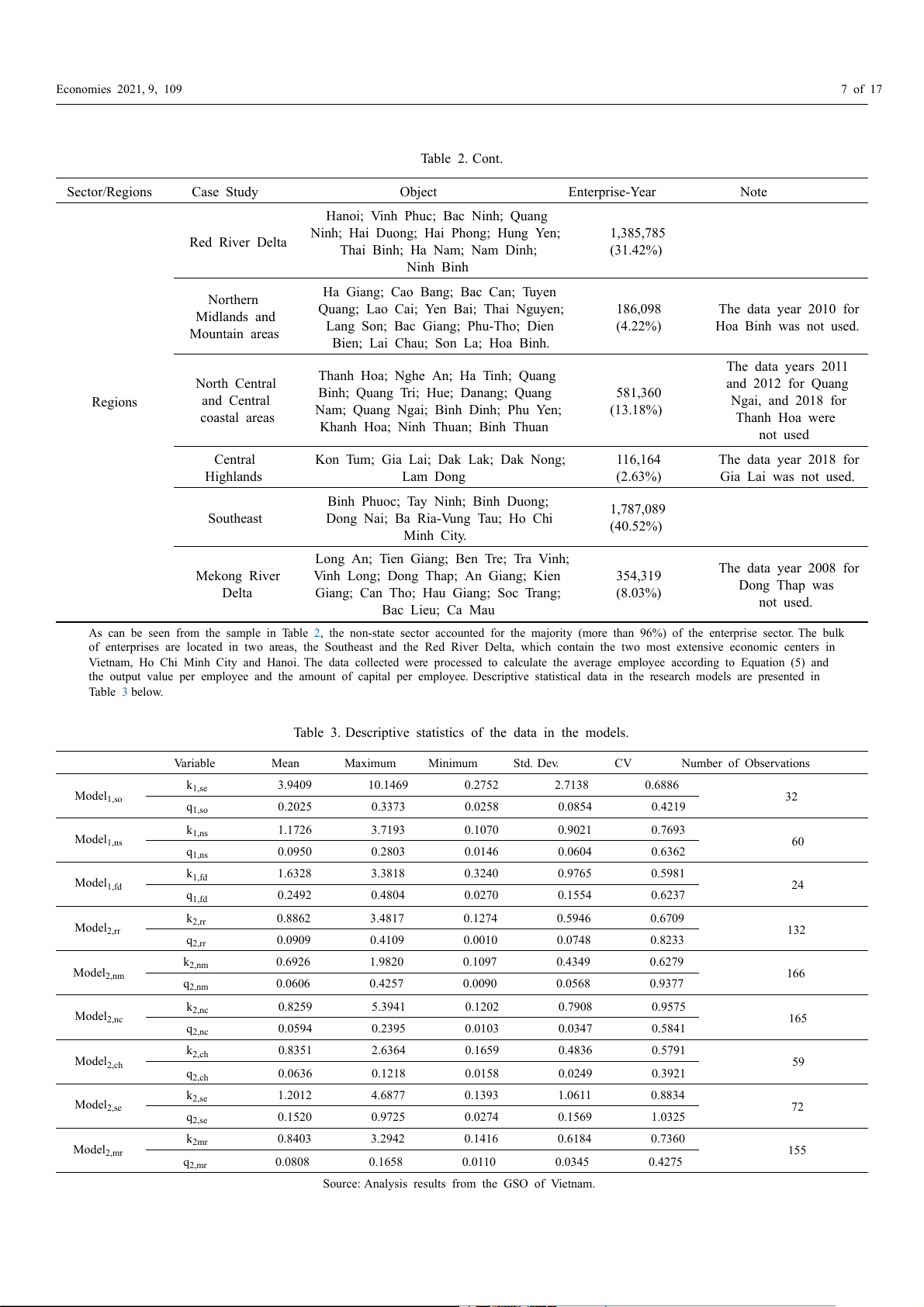
enterprises joint ventures with (2.75%) enterprise sector foreign parties. Economies 2021, 9, 109 7 of 17 Table 2. Cont. Sector/Regions Case Study Object Enterprise-Year Note
Hanoi; Vinh Phuc; Bac Ninh; Quang
Ninh; Hai Duong; Hai Phong; Hung Yen; 1,385,785 Red River Delta Thai Binh; Ha Nam; Nam Dinh; (31.42%) Ninh Binh
Ha Giang; Cao Bang; Bac Can; Tuyen Northern
Quang; Lao Cai; Yen Bai; Thai Nguyen; 186,098 The data year 2010 for Midlands and
Lang Son; Bac Giang; Phu-Tho; Dien (4.22%) Hoa Binh was not used. Mountain areas
Bien; Lai Chau; Son La; Hoa Binh. The data years 2011
Thanh Hoa; Nghe An; Ha Tinh; Quang North Central and 2012 for Quang
Binh; Quang Tri; Hue; Danang; Quang 581,360 Regions and Central Ngai, and 2018 for
Nam; Quang Ngai; Bình Dinh; Phu Yen; (13.18%) coastal areas Thanh Hoa were
Khanh Hoa; Ninh Thuan; Binh Thuan not used Central
Kon Tum; Gia Lai; Dak Lak; Dak Nong; 116,164 The data year 2018 for Highlands Lam Dong (2.63%) Gia Lai was not used.
Binh Phuoc; Tay Ninh; Binh Duong; 1,787,089 Southeast
Dong Nai; Ba Ria-Vung Tau; Ho Chi (40.52%) Minh City.
Long An; Tien Giang; Ben Tre; Tra Vinh; The data year 2008 for Mekong River
Vinh Long; Dong Thap; An Giang; Kien 354,319 Dong Thap was Delta
Giang; Can Tho; Hau Giang; Soc Trang; (8.03%) not used. Bac Lieu; Ca Mau
As can be seen from the sample in Table 2, the non-state sector accounted for the majority (more than 96%) of the enterprise sector. The bulk
of enterprises are located in two areas, the Southeast and the Red River Delta, which contain the two most extensive economic centers in
Vietnam, Ho Chi Minh City and Hanoi. The data collected were processed to calculate the average employee according to Equation (5) and
the output value per employee and the amount of capital per employee. Descriptive statistical data in the research models are presented in Table 3 below.
Table 3. Descriptive statistics of the data in the models. Variable Mean Maximum Minimum Std. Dev. CV Number of Observations k1,se 3.9409 10.1469 0.2752 2.7138 0.6886 Model1,so 32 q1,so 0.2025 0.3373 0.0258 0.0854 0.4219 k Model 1,ns 1.1726 3.7193 0.1070 0.9021 0.7693 1,ns 60 q1,ns 0.0950 0.2803 0.0146 0.0604 0.6362 k Model 1,fd 1.6328 3.3818 0.3240 0.9765 0.5981 1,fd 24 q1,fd 0.2492 0.4804 0.0270 0.1554 0.6237 k Model 2,rr 0.8862 3.4817 0.1274 0.5946 0.6709 2,rr 132 q2,rr 0.0909 0.4109 0.0010 0.0748 0.8233 k2,nm 0.6926 1.9820 0.1097 0.4349 0.6279 Model2,nm 166 q2,nm 0.0606 0.4257 0.0090 0.0568 0.9377 k Model 2,nc 0.8259 5.3941 0.1202 0.7908 0.9575 2,nc 165 q2,nc 0.0594 0.2395 0.0103 0.0347 0.5841 k2,ch 0.8351 2.6364 0.1659 0.4836 0.5791 Model2,ch 59 q2,ch 0.0636 0.1218 0.0158 0.0249 0.3921 k Model 2,se 1.2012 4.6877 0.1393 1.0611 0.8834 2,se 72 q2,se 0.1520 0.9725 0.0274 0.1569 1.0325 k2mr 0.8403 3.2942 0.1416 0.6184 0.7360 Model2,mr 155 q2,mr 0.0808 0.1658 0.0110 0.0345 0.4275
Source: Analysis results from the GSO of Vietnam. Economies 2021, 9, 109 8 of 17
4. Research Results and Discussion
4.1. Unit Root Test and Cointegration Test
Panel unit root tests were conducted for all three patterns. These included a trend and
an intercept exists, only an intercept exists, or neither exists using the testing methods of
Im, Pesaran and Shin (IPS), Fisher type test using Augmented Dickey–Fuller (ADF), and
the Philips Perron (PP) test. These unit root tests are appropriate methods for unbalanced
panel data. The lag length was automatically chosen by the Schwarz Information Criterion
(SIC) with Newey–West automatic bandwidth selection and Bartlett kernel. The panel unit
root test results are represented in the Appendix A. According to the results of the unit root
test, the series are stationary at different level for each test of each pattern, but there is at
least one series that is not stationary at level, so that OLS estimation might be a spurious
regression (Granger and Newbold 1974). Under these circumstances, a cointegration test
was conducted to evaluate the long-term relationship among variables. According to
Pedroni (1999), there are seven test statistics to analyze the cointegration relation among
the variables in a panel data model where the null hypothesis of no cointegration has
been formulated. Additionally, the Kao test (developed by Kao 1999), which has the null
hypothesis of no cointegration, was utilized to assess the cointegration relation. The results
of the panel cointegration test for each model are presented in the Appendix A. The first
test performed was the Pedroni test. The results for at least 4/7 tests were statistically
significant at either 0.05 or 0.01 level in both “Individual Intercept” and “Individual
Intercept and Individual trend” for most models, except for model 1,ns , model1,fd , and
model 2,se. In other words, most of the tests achieve statistical significance at the 0.01 or
0.05 level for these models. Model1,ns and model 1,fd produced the most test results (at
least 4/7), which were statistically significant at 0.01 or 0.05 level for “Individual Intercept”
but for “Individual Intercept and Individual trend”, they do not meet this requirement.
By contrast, in model2,se , although 5/7 tests that are statistically significant at 0.01 or 0.05
level for the case of “Individual Intercept and Individual trend”, there are only 2/7 tests
statistically significant at the 0.01 or 0.05 level for “Individual Intercept”. Therefore, the
Pedroni test cannot reject the null hypothesis for models 1,ns, models 1,fd , and models2,se,
where the Kao test was conducted.
The Kao test results for these models in the Appendix A all produce relatively large
t-Statistic values with significance at the 0.01 or 0.05 level. Thus, with the Pedroni test, as
supplemented by the Kao test, it is possible to accept alternative hypotheses for all models.
This means that the variables in all models are long-run associated.
4.2. The Results of the Parameter Estimation
Due to the cointegration relationship between the variables in the models, parameters
can be estimated by cointegrating regression for panel data, such as by fully modified
ordinary least squares (FMOLS) or dynamic ordinary least squares (DOLS). This study
chose the FMOLS method because there is a large variation in the long-term coefficients of
variance among the objects of the panel data (type of enterprise in sectors or enterprise in
provinces within regions). The estimated results of the parameters in the models where the
FMOLS method was applied are presented in Table 4 below.
Table 4 above shows a greater than 50% adjusted R2 for all models. As the standard
errors are quite small, the regression models are appropriate and accepted. The estimated
parameters ( α ) in all models have quite large T-statistic values with statistical significance
at the 1% level, except for model2,mr at 5% level, so the parameters are accepted. Thus, the
estimated values of the parameters are in the range of 0 to 1. According to the estimation
results, the role of capital is higher than that of labor in all enterprise sectors. The greatest
leverage is the foreign investment enterprise sector, followed by the non-state enterprise
sector and finally, the state-owned enterprise sector. For regions, the role of capital is
substantially greater than that of labor, except for region 3 (North Central and Central
Coastal areas). The most prominent is region 1 (Red River Delta), the next is region 5 Economies 2021, 9, 109 9 of 17
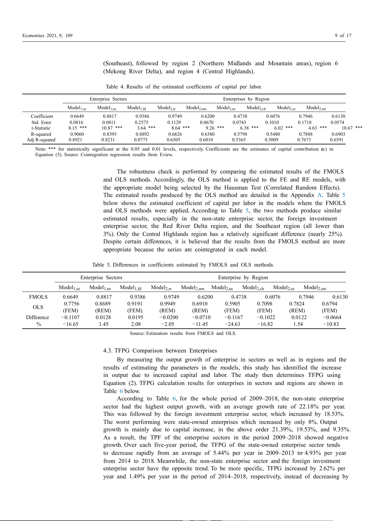
(Southeast), followed by region 2 (Northern Midlands and Mountain areas), region 6
(Mekong River Delta), and region 4 (Central Highlands).
Table 4. Results of the estimated coefficients of capital per labor. Enterprise Sectors Enterprises by Region Model1,se Model1,ns Model1,fd Model2,rr Model2,nm Model2,nc Model2,ch Model2,se Model2,mr Coefficient 0.6649 0.8817 0.9386 0.9749 0.6200 0.4738 0.6076 0.7946 0.6130 Std. Error 0.0816 0.0811 0.2575 0.1129 0.0670 0.0743 0.1010 0.1718 0.0574 t-Statistic 8.15 *** 10.87 *** 3.64 *** 8.64 *** 9.26 *** 6.38 *** 6.02 *** 4.63 *** 10.67 *** R-squared 0.9060 0.8395 0.8892 0.6826 0.6380 0.5798 0.5480 0.7888 0.6903 Adj R-squared 0.8921 0.8231 0.8775 0.6505 0.6010 0.5365 0.5009 0.7673 0.6591
Note: *** for statistically significant at the 0.05 and 0.01 levels, respectively. Coefficients are the estimates of capital contribution (α) in
Equation (5). Source: Cointegration regression results from Eview.
The robustness check is performed by comparing the estimated results of the FMOLS
and OLS methods. Accordingly, the OLS method is applied to the FE and RE models, with
the appropriate model being selected by the Hausman Test (Correlated Random Effects).
The estimated results produced by the OLS method are detailed in the Appendix A. Table 5
below shows the estimated coefficient of capital per labor in the models where the FMOLS
and OLS methods were applied. According to Table 5, the two methods produce similar
estimated results, especially in the non-state enterprise sector, the foreign investment
enterprise sector, the Red River Delta region, and the Southeast region (all lower than
3%). Only the Central Highlands region has a relatively significant difference (nearly 25%).
Despite certain differences, it is believed that the results from the FMOLS method are more
appropriate because the series are cointegrated in each model.
Table 5. Differences in coefficients estimated by FMOLS and OLS methods. Enterprise Sectors Enterprise by Region Model1,se Model1,ns Model1,fd Model2,rr Model2,nm Model2,nc Model2,ch Model2,se Model2,mr FMOLS 0.6649 0.8817 0.9386 0.9749 0.6200 0.4738 0.6076 0.7946 0.6130 0.7756 0.8689 0.9191 0.9949 0.6910 0.5905 0.7098 0.7824 0.6794 OLS (FEM) (REM) (FEM) (REM) (REM) (FEM) (FEM) (REM) (FEM) Difference −0.1107 0.0128 0.0195 −0.0200 −0.0710 −0.1167 −0.1022 0.0122 −0.0664 % −16.65 1.45 2.08 −2.05 −11.45 −24.63 −16.82 1.54 −10.83
Source: Estimation results from FMOLS and OLS.
4.3. TFPG Comparison between Enterprises
By measuring the output growth of enterprise in sectors as well as in regions and the
results of estimating the parameters in the models, this study has identified the increase
in output due to increased capital and labor. The study then determines TFPG using
Equation (2). TFPG calculation results for enterprises in sectors and regions are shown in Table 6 below.
According to Table 6, for the whole period of 2009–2018, the non-state enterprise
sector had the highest output growth, with an average growth rate of 22.18% per year.
This was followed by the foreign investment enterprise sector, which increased by 18.53%.
The worst performing were state-owned enterprises which increased by only 8%. Output
growth is mainly due to capital increase, in the above order 21.39%, 19.53%, and 9.35%.
As a result, the TPF of the enterprise sectors in the period 2009–2018 showed negative
growth. Over each five-year period, the TFPG of the state-owned enterprise sector tends
to decrease rapidly from an average of 5.44% per year in 2009–2013 to− 4.93% per year
from 2014 to 2018. Meanwhile, the non-state enterprise sector and the foreign investment
enterprise sector have the opposite trend. To be more specific, TFPG increased by 2.62% per
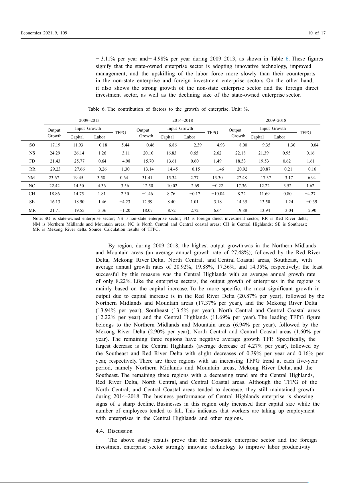
year and 1.49% per year in the period of 2014–2018, respectively, instead of decreasing by Economies 2021, 9, 109 10 of 17
− 3.11% per year and− 4.98% per year during 2009–2013, as shown in Table 6. These figures
signify that the state-owned enterprise sector is adopting innovative technology, improved
management, and the upskilling of the labor force more slowly than their counterparts
in the non-state enterprise and foreign investment enterprise sectors. On the other hand,
it also shows the strong growth of the non-state enterprise sector and the foreign direct
investment sector, as well as the declining size of the state-owned enterprise sector.
Table 6. The contribution of factors to the growth of enterprise. Unit: %. 2009–2013 2014–2018 2009–2018 Output Input Growth Output Input Growth Output Input Growth TFPG TFPG TFPG Growth Growth Growth Capital Labor Capital Labor Capital Labor SO 17.19 11.93 −0.18 5.44 −0.46 6.86 −2.39 −4.93 8.00 9.35 −1.30 −0.04 NS 24.29 26.14 1.26 −3.11 20.10 16.83 0.65 2.62 22.18 21.39 0.95 −0.16 FD 21.43 25.77 0.64 −4.98 15.70 13.61 0.60 1.49 18.53 19.53 0.62 −1.61 RR 29.23 27.66 0.26 1.30 13.14 14.45 0.15 −1.46 20.92 20.87 0.21 −0.16 NM 23.67 19.45 3.58 0.64 31.41 15.34 2.77 13.30 27.48 17.37 3.17 6.94 NC 22.42 14.50 4.36 3.56 12.50 10.02 2.69 −0.22 17.36 12.22 3.52 1.62 CH 18.86 14.75 1.81 2.30 −1.46 8.76 −0.17 −10.04 8.22 11.69 0.80 −4.27 SE 16.13 18.90 1.46 −4.23 12.59 8.40 1.01 3.18 14.35 13.50 1.24 −0.39 MR 21.71 19.55 3.36 −1.20 18.07 8.72 2.72 6.64 19.88 13.94 3.04 2.90
Note: SO is state-owned enterprise sector; NS is non-state enterprise sector; FD is foreign direct investment sector; RR is Red River delta;
NM is Northern Midlands and Mountain areas; NC is North Central and Central coastal areas; CH is Central Highlands; SE is Southeast;
MR is Mekong River delta. Source: Calculation results of TFPG.
By region, during 2009–2018, the highest output growth was in the Northern Midlands
and Mountain areas (an average annual growth rate of 27.48%); followed by the Red River
Delta, Mekong River Delta, North Central, and Central Coastal areas, Southeast, with
average annual growth rates of 20.92%, 19.88%, 17.36%, and 14.35%, respectively; the least
successful by this measure was the Central Highlands with an average annual growth rate
of only 8.22%. Like the enterprise sectors, the output growth of enterprises in the regions is
mainly based on the capital increase. To be more specific, the most significant growth in
output due to capital increase is in the Red River Delta (20.87% per year), followed by the
Northern Midlands and Mountain areas (17.37% per year), and the Mekong River Delta
(13.94% per year), Southeast (13.5% per year), North Central and Central Coastal areas
(12.22% per year) and the Central Highlands (11.69% per year). The leading TFPG figure
belongs to the Northern Midlands and Mountain areas (6.94% per year), followed by the
Mekong River Delta (2.90% per year), North Central and Central Coastal areas (1.60% per
year). The remaining three regions have negative average growth TFP. Specifically, the
largest decrease is the Central Highlands (average decrease of 4.27% per year), followed by
the Southeast and Red River Delta with slight decreases of 0.39% per year and 0.16% per
year, respectively. There are three regions with an increasing TFPG trend at each five-year
period, namely Northern Midlands and Mountain areas, Mekong River Delta, and the
Southeast. The remaining three regions with a decreasing trend are the Central Highlands,
Red River Delta, North Central, and Central Coastal areas. Although the TFPG of the
North Central, and Central Coastal areas tended to decrease, they still maintained growth
during 2014–2018. The business performance of Central Highlands enterprise is showing
signs of a sharp decline. Businesses in this region only increased their capital size while the
number of employees tended to fall. This indicates that workers are taking up employment
with enterprises in the Central Highlands and other regions. 4.4. Discussion
The above study results prove that the non-state enterprise sector and the foreign
investment enterprise sector strongly innovate technology to improve labor productivity Economies 2021, 9, 109 11 of 17
more than the state-owned enterprise sector. These results are consistent with some
recent studies demonstrating that foreign direct investment enterprises in Vietnam have
an expanding role in TFP (Hien et al. 2019); and negative TFP growth of state-owned
enterprises in China (Ozyurt 2009). The results also support the outcome of the study
by Le et al. (2021), which argues that state ownership is negatively associated with TFP.
The decline in TFPG is because enterprises in the state-owned sector remain inefficient,
have fewer incentives to change and change management. In addition, the study by
Le et al. (2021)also shows that corruption control hinders TFP. It should be noted that
during the last three decades of reforms, state-owned enterprises have been reformed, many
privileges of the state-owned enterprises have been removed and the least efficient were
merged or equitized. However, the results of this study cast doubt about the effectiveness
of state-own enterprise reform measures in Vietnam.
The relatively stable TFPG of the non-state enterprise sector during 2009–2018 found
in this study is evidence that lends support to the view that the private sector is increasingly
effective and plays an important role in the economic development of Vietnam. One of
these reasons was studied by Le et al. (2021). They indicated that transparency promotes
the TFP of private enterprises more than that of state-owned enterprises. In addition, in
Vietnam, small and medium-sized enterprises are mainly in the non-state sector (between
2005 and 2018, the non-state enterprise sector accounted for 96.41% of the number of
enterprises but only 59.13% of the labor and 50.83% of the capital). Hence, the TFPG of the
non-state sector partly reflects the efficiency of small and medium-sized enterprises. The
TFPG of the non-state sector found in this study is also consistent with the research results
of Hue et al. (2019), which indicated that innovation has a positive impact on the TFP of
small and medium-sized enterprises in Vietnam.
TFPG differences between regions of any country are apparent, but this study has
shown specific differences between six regions in Vietnam by analyzing data up to 2018.
It is believed that no previous studies have conducted this type of analysis. To be more
specific, the Northern Midlands and Mountain areas and the Mekong River Delta are
developing well as these regions increased their TFPG during 2009–2018 as well as in
2014–2018 and 2009–2013. This could be a sign of their emerging status as economic zones.
North Central and Central Coastal areas, and the Southeast, although still maintaining
TFPG growth, are experiencing slower growth rates. Meanwhile, the TFPG of the Red
River Delta and the Central Highlands has ceased growth and is now dipping downwards.
This trend is especially marked in the Central Highlands, where workers move away to
find employment in other regions. Despite efforts to combat the outward labor migration
and increase agricultural employment, negative growth persists. The reason for this
phenomenon is because most provinces in this region are slow to develop, have poor
transportation infrastructure, have few industrial zones, and the pace of industrialization
and urbanization is relative slow. These findings, therefore, illustrate the unbalanced
development of TFP among the regions of Vietnam.
The growth models indicate the vital role of capital in the foreign direct investment
enterprise, non-state enterprise sectors as well as enterprises in the region of the Red River
Delta and the Southeast. Vietnamese enterprises have seen output value growth in recent
years, mainly thanks to capital increase. This is especially the case in the non-state sector,
the foreign investment sector as well as the Red River Delta, and Northern Midlands and
Mountain areas. Two main factors can explain this. First, it is derived from the roles of
capital and labor as in the model estimates above. Second, increasing labor will be limited
at the macro level because human social resources are limited and hampered by slow
growth, while raising capital will face fewer obstacles.
5. Conclusions and Implications
This study has identified and compared TFPG among enterprise sectors and enter-
prises in different regions in Vietnam by using the parametric approach with two input
variables, capital and labor. Based on cointegrating regression analysis techniques for panel Economies 2021, 9, 109 12 of 17
data, the study has found evidence of the different roles of capital and labor in the output
of the enterprise sectors as well as individual enterprises within different regions. The
role of capital to output growth in the foreign investment sector is the most prominent,
followed by the non-state enterprise sector and finally, the state-owned enterprise sector.
The foremost capital beneficiary is the Red River Delta, then the Southeast, the Northern
Midlands and Mountain areas, followed by the Mekong River Delta, Central Highlands,
and the North Central and Central Coastal areas. On the other hand, the contribution of
labor toward the output growth rate of enterprise sectors and enterprises in regions is the
opposite of capital contribution. In the period 2009–2018, the growth of output value (profit
before tax and income of employees) of Vietnamese enterprises was mainly attributed to
the capital increase, especially in the non-state enterprise sector and the Red River Delta.
Indeed, the growth of the state-owned enterprise sector was entirely funded by capital
during 2009–2018, and this is also found to hold in the Central Highlands during the period 2014–2018.
Besides the role of capital and labor, which indicate an enterprise’s efficiency and
productivity, this study also shows that TFP plays a key role in increasing the output
volume of Vietnamese enterprises. From 2009 to 2018, there was a stark contrast in TFPG in
terms of value and changing trends between enterprise sectors and individual enterprises
within regions. In the five years 2014–2018, only the non-state enterprise sector and the
foreign direct investment sector had TFP growth, but the state-owned enterprise sector
fell sharply. The TFP of the Northern Midlands and Mountain areas, the Mekong River
Delta, and the Southeast also trended toward growth. Meanwhile, the TFP of the Central
Highlands and the Red River Delta tended to decrease and grow negatively in the period
2009–2018, especially in the Central Highlands. Although tending to decrease slightly, the
TFP of the North Central and Central Coastal areas still maintained a positive growth rate
during 2009–2018. These findings demonstrate the weakness of the state-owned enterprise
sector and the increasing efficiency of the non-state enterprise sector and the foreign direct
investment enterprise sector. The unbalanced development of TFPG among regions found
in this study is indicative of the growing economic gap among regions. This is a scenario
not usually expected internationally but for Vietnam is a case in point.
The results of this study imply that the government should continue to push ahead
with reforms to improve the efficiency of state-owned enterprises. Although the state-
owned sector accounts for only 0.84% of enterprises, they provide 14.01% of labor and
31.33% of capital in active enterprises. Therefore, they still play an important role in
maintaining the state-owned sector and remain necessary. However, the state only needs
to hold key areas to ensure social cohesion that other sectors do not want to participate in,
such as reducing state ownership and loosening administrative controls. In addition, the
state continues to create mechanisms to promote the non-state enterprise sector and foreign
direct investment enterprise sector, creating a level playing field for all types of enterprises.
In order to reduce the economic gap between regions, the state also needs to have policies
to support underdeveloped enterprise areas, declining TFPG, especially in the Central
Highlands, such as infrastructure development, policies to support capital and training,
and so on. Addressing these issues would help the regions create advantageous conditions
for production and business, innovation management, and technology to improve TFP. On
their side, enterprises need to focus on increasing capital for growth and development,
especially innovating and improving technology and management methods to promote
TFPG. Capital increases will be more favorable than labor growth because, from a social
perspective, the ability to increase labor will be limited. However, innovation in technology
and management to increase TFP is the central issue to improve the efficiency of enterprises.
The contribution of this study can be considered in two ways. First, academically, this
study enriches the method of estimating capital and labor contribution coefficients by
cointegration regression analysis for panel data. Second, in practical terms, this study shows
the different roles of capital, labor, and TFPG in increasing the output of the enterprise
sectors and enterprises in different regions of Vietnam. Furthermore, the study’s findings on Economies 2021, 9, 109 13 of 17
unbalanced development within sectors and regions form the basis to build an appropriate policy mix.
Although this study has obtained some valuable results, some limitations should
be noted. Firstly, due to data limitations, this study only explores TFPG from a macro
perspective, such as among sectors and regions, without analyzing the internal perfor-
mance of each specific industry. Secondly, due to the macro perspective, this study only
considers two inputs when studying each specific industry, so the input factors need to be
supplemented accordingly. Nevertheless, these issues may still provide opportunities for further study.
Funding: This research was funded by University of Economics and Law, Vietnam National Univer-
sity, Ho Chi Minh, Vietnam, under grant number 2-2021.
Institutional Review Board Statement: Not applicable.
Informed Consent Statement: Not applicable. Data Availability Statement:
Data are available in the GSO statistical yearbooks, accessible from:
http://thongke.gov.vn/default.aspx?tabid=512&idmid=5&ItemID=11973; http://thongke.gov.vn/
default.aspx?tabid=512&idmid=5&ItemID=12574; http://thongke.gov.vn/default.aspx?tabid=512&
idmid=5&ItemID=13760; http://thongke.gov.vn/default.aspx?tabid=512&idmid=5&ItemID=14080;
http://thongke.gov.vn/default.aspx?tabid=512&idmid=5&ItemID=15161; http://thongke.gov.vn/
default.aspx?tabid=512&idmid=5&ItemID=16051; http://thongke.gov.vn/default.aspx?tabid=512&
idmid=5&ItemID=18531; http://thongke.gov.vn/default.aspx?tabid=512&idmid=5&ItemID=18940;
http://thongke.gov.vn/default.aspx?tabid=512&idmid=5&ItemID=19298. Acknowledgments:
The author is grateful to the four anonymous reviewers and Academic Editor
whose comments have contributed to improving the quality of this paper.
Conflicts of Interest: The authors declare no conflict of interest. Appendix A Appendix A.1. Unit Root Test
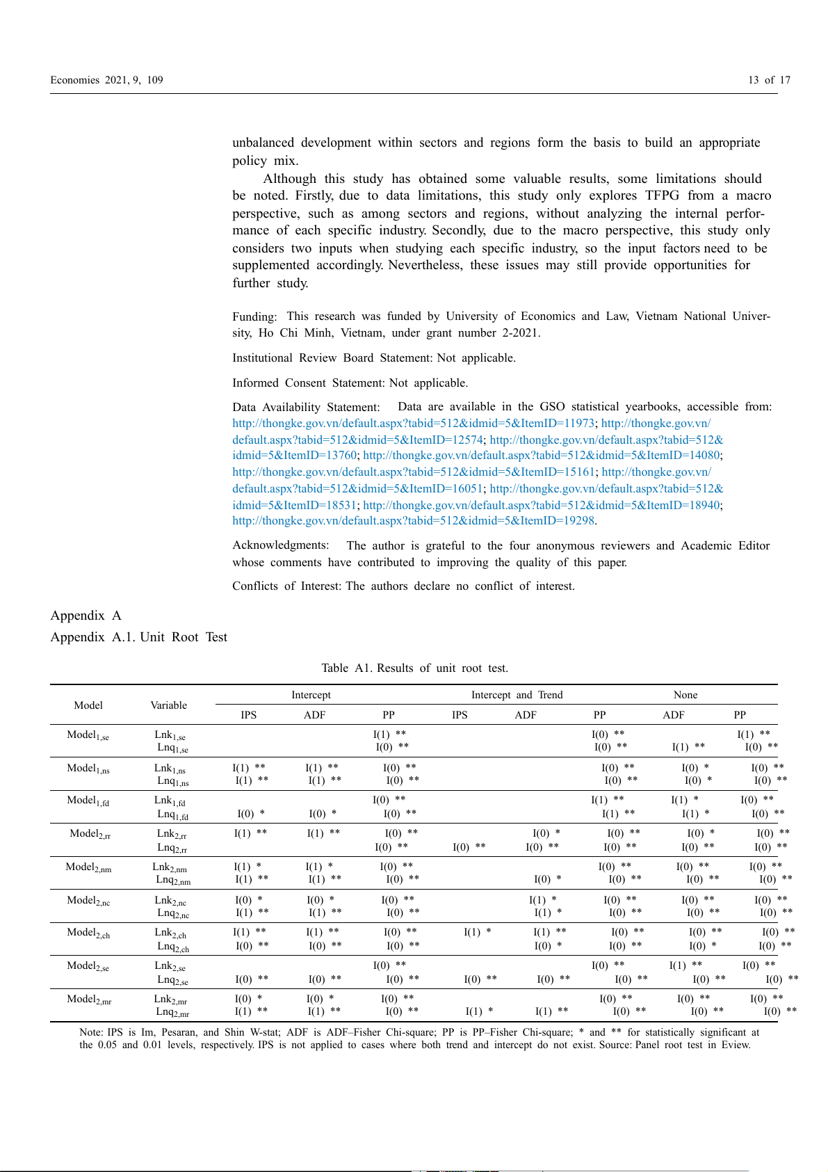
Table A1. Results of unit root test. Intercept Intercept and Trend None Model Variable IPS ADF PP IPS ADF PP ADF PP Model1,se Lnk1,se I(1) ** I(0) ** I(1) ** Lnq1,se I(0) ** I(0) ** I(1) ** I(0) ** Model1,ns Lnk1,ns I(1) ** I(1) ** I(0) ** I(0) ** I(0) * I(0) ** Lnq1,ns I(1) ** I(1) ** I(0) ** I(0) ** I(0) * I(0) ** Model1,fd Lnk1,fd I(0) ** I(1) ** I(1) * I(0) ** Lnq1,fd I(0) * I(0) * I(0) ** I(1) ** I(1) * I(0) ** Model2,rr Lnk2,rr I(1) ** I(1) ** I(0) ** I(0) * I(0) ** I(0) * I(0) ** Lnq2,rr I(0) ** I(0) ** I(0) ** I(0) ** I(0) ** I(0) ** Model2,nm Lnk2,nm I(1) * I(1) * I(0) ** I(0) ** I(0) ** I(0) ** Lnq2,nm I(1) ** I(1) ** I(0) ** I(0) * I(0) ** I(0) ** I(0) ** Model2,nc Lnk2,nc I(0) * I(0) * I(0) ** I(1) * I(0) ** I(0) ** I(0) ** Lnq2,nc I(1) ** I(1) ** I(0) ** I(1) * I(0) ** I(0) ** I(0) ** Model2,ch Lnk2,ch I(1) ** I(1) ** I(0) ** I(1) * I(1) ** I(0) ** I(0) ** I(0) ** Lnq2,ch I(0) ** I(0) ** I(0) ** I(0) * I(0) ** I(0) * I(0) ** Model2,se Lnk2,se I(0) ** I(0) ** I(1) ** I(0) ** Lnq2,se I(0) ** I(0) ** I(0) ** I(0) ** I(0) ** I(0) ** I(0) ** I(0) ** Model2,mr Lnk2,mr I(0) * I(0) * I(0) ** I(0) ** I(0) ** I(0) ** Lnq2,mr I(1) ** I(1) ** I(0) ** I(1) * I(1) ** I(0) ** I(0) ** I(0) **
Note: IPS is Im, Pesaran, and Shin W-stat; ADF is ADF–Fisher Chi-square; PP is PP–Fisher Chi-square; * and ** for statistically significant at
the 0.05 and 0.01 levels, respectively. IPS is not applied to cases where both trend and intercept do not exist. Source: Panel root test in Eview. Economies 2021, 9, 109 14 of 17
Appendix A.2. Panel Cointegration Analysis
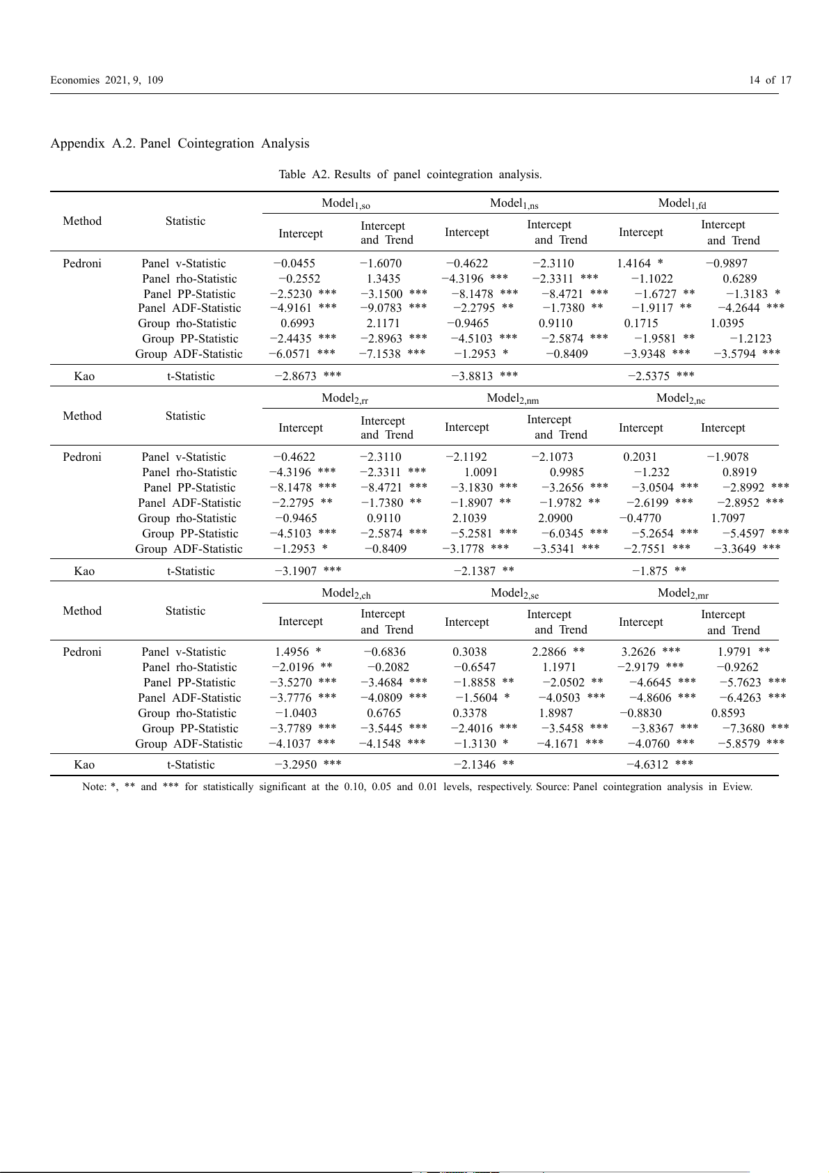
Table A2. Results of panel cointegration analysis. Model1,so Model1,ns Model1,fd Method Statistic Intercept Intercept Intercept Intercept Intercept Intercept and Trend and Trend and Trend Pedroni Panel v-Statistic −0.0455 −1.6070 −0.4622 −2.3110 1.4164 * −0.9897 Panel rho-Statistic −0.2552 1.3435 −4.3196 *** −2.3311 *** −1.1022 0.6289 Panel PP-Statistic −2.5230 *** −3.1500 *** −8.1478 *** −8.4721 *** −1.6727 ** −1.3183 * Panel ADF-Statistic −4.9161 *** −9.0783 *** −2.2795 ** −1.7380 ** −1.9117 ** −4.2644 *** Group rho-Statistic 0.6993 2.1171 −0.9465 0.9110 0.1715 1.0395 Group PP-Statistic −2.4435 *** −2.8963 *** −4.5103 *** −2.5874 *** −1.9581 ** −1.2123 Group ADF-Statistic −6.0571 *** −7.1538 *** −1.2953 * −0.8409 −3.9348 *** −3.5794 *** Kao t-Statistic −2.8673 *** −3.8813 *** −2.5375 *** Model2,rr Model2,nm Model2,nc Method Statistic Intercept Intercept Intercept Intercept Intercept Intercept and Trend and Trend Pedroni Panel v-Statistic −0.4622 −2.3110 −2.1192 −2.1073 0.2031 −1.9078 Panel rho-Statistic −4.3196 *** −2.3311 *** 1.0091 0.9985 −1.232 0.8919 Panel PP-Statistic −8.1478 *** −8.4721 *** −3.1830 *** −3.2656 *** −3.0504 *** −2.8992 *** Panel ADF-Statistic −2.2795 ** −1.7380 ** −1.8907 ** −1.9782 ** −2.6199 *** −2.8952 *** Group rho-Statistic −0.9465 0.9110 2.1039 2.0900 −0.4770 1.7097 Group PP-Statistic −4.5103 *** −2.5874 *** −5.2581 *** −6.0345 *** −5.2654 *** −5.4597 *** Group ADF-Statistic −1.2953 * −0.8409 −3.1778 *** −3.5341 *** −2.7551 *** −3.3649 *** Kao t-Statistic −3.1907 *** −2.1387 ** −1.875 ** Model2,ch Model2,se Model2,mr Method Statistic Intercept Intercept Intercept Intercept Intercept Intercept and Trend and Trend and Trend Pedroni Panel v-Statistic 1.4956 * −0.6836 0.3038 2.2866 ** 3.2626 *** 1.9791 ** Panel rho-Statistic −2.0196 ** −0.2082 −0.6547 1.1971 −2.9179 *** −0.9262 Panel PP-Statistic −3.5270 *** −3.4684 *** −1.8858 ** −2.0502 ** −4.6645 *** −5.7623 *** Panel ADF-Statistic −3.7776 *** −4.0809 *** −1.5604 * −4.0503 *** −4.8606 *** −6.4263 *** Group rho-Statistic −1.0403 0.6765 0.3378 1.8987 −0.8830 0.8593 Group PP-Statistic −3.7789 *** −3.5445 *** −2.4016 *** −3.5458 *** −3.8367 *** −7.3680 *** Group ADF-Statistic −4.1037 *** −4.1548 *** −1.3130 * −4.1671 *** −4.0760 *** −5.8579 *** Kao t-Statistic −3.2950 *** −2.1346 ** −4.6312 ***
Note: *, ** and *** for statistically significant at the 0.10, 0.05 and 0.01 levels, respectively. Source: Panel cointegration analysis in Eview. Economies 2021, 9, 109 15 of 17
Appendix A.3. Estimation by OLS Method
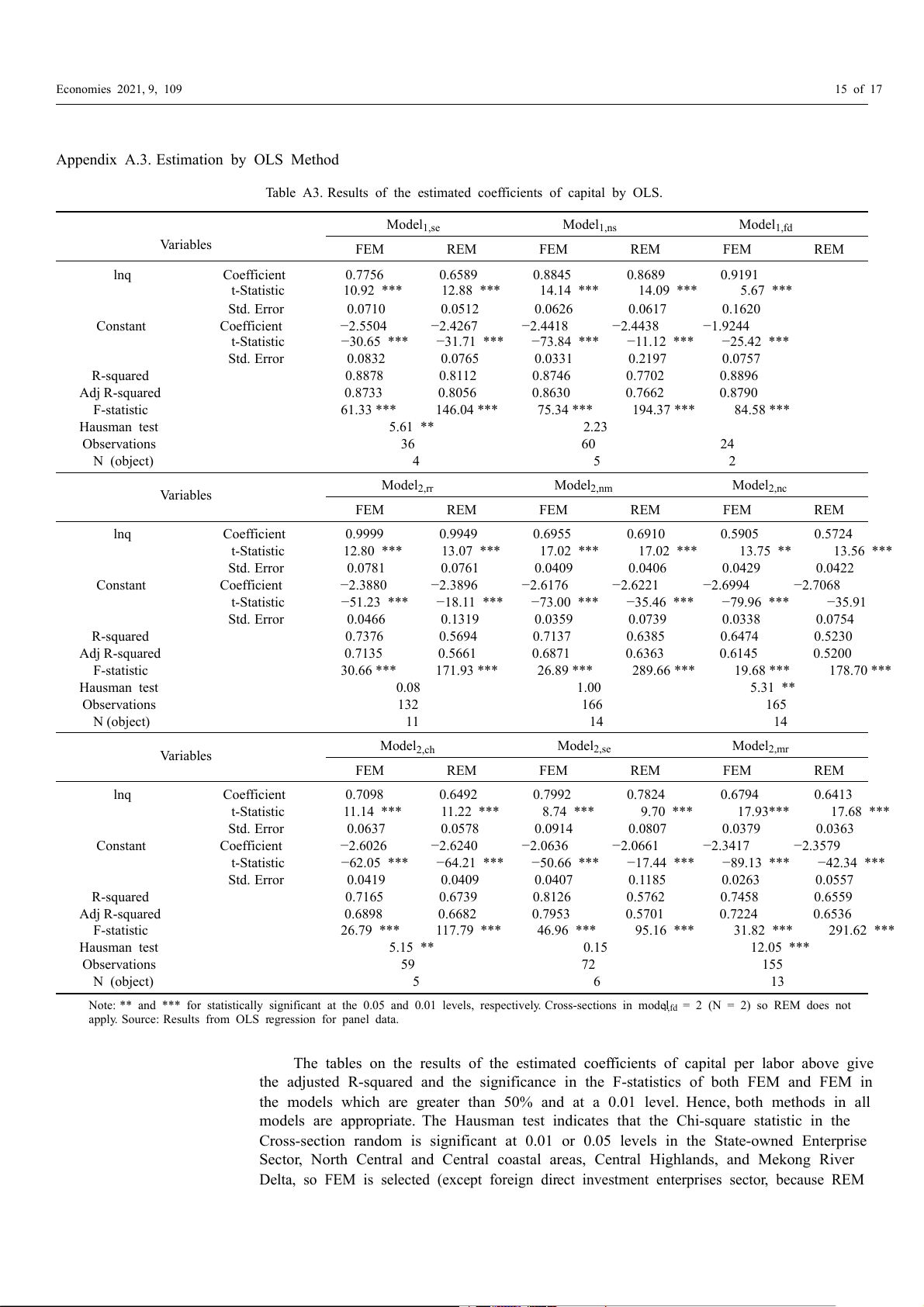
Table A3. Results of the estimated coefficients of capital by OLS. Model1,se Model1,ns Model1,fd Variables FEM REM FEM REM FEM REM lnq Coefficient 0.7756 0.6589 0.8845 0.8689 0.9191 t-Statistic 10.92 *** 12.88 *** 14.14 *** 14.09 *** 5.67 *** Std. Error 0.0710 0.0512 0.0626 0.0617 0.1620 Constant Coefficient −2.5504 −2.4267 −2.4418 −2.4438 −1.9244 t-Statistic −30.65 *** −31.71 *** −73.84 *** −11.12 *** −25.42 *** Std. Error 0.0832 0.0765 0.0331 0.2197 0.0757 R-squared 0.8878 0.8112 0.8746 0.7702 0.8896 Adj R-squared 0.8733 0.8056 0.8630 0.7662 0.8790 F-statistic 61.33 *** 146.04 *** 75.34 *** 194.37 *** 84.58 *** Hausman test 5.61 ** 2.23 Observations 36 60 24 N (object) 4 5 2 Model Variables 2,rr Model2,nm Model2,nc FEM REM FEM REM FEM REM lnq Coefficient 0.9999 0.9949 0.6955 0.6910 0.5905 0.5724 t-Statistic 12.80 *** 13.07 *** 17.02 *** 17.02 *** 13.75 ** 13.56 *** Std. Error 0.0781 0.0761 0.0409 0.0406 0.0429 0.0422 Constant Coefficient −2.3880 −2.3896 −2.6176 −2.6221 −2.6994 −2.7068 t-Statistic −51.23 *** −18.11 *** −73.00 *** −35.46 *** −79.96 *** −35.91 Std. Error 0.0466 0.1319 0.0359 0.0739 0.0338 0.0754 R-squared 0.7376 0.5694 0.7137 0.6385 0.6474 0.5230 Adj R-squared 0.7135 0.5661 0.6871 0.6363 0.6145 0.5200 F-statistic 30.66 *** 171.93 *** 26.89 *** 289.66 *** 19.68 *** 178.70 *** Hausman test 0.08 1.00 5.31 ** Observations 132 166 165 N (object) 11 14 14 Model Variables 2,ch Model2,se Model2,mr FEM REM FEM REM FEM REM lnq Coefficient 0.7098 0.6492 0.7992 0.7824 0.6794 0.6413 t-Statistic 11.14 *** 11.22 *** 8.74 *** 9.70 *** 17.93*** 17.68 *** Std. Error 0.0637 0.0578 0.0914 0.0807 0.0379 0.0363 Constant Coefficient −2.6026 −2.6240 −2.0636 −2.0661 −2.3417 −2.3579 t-Statistic −62.05 *** −64.21 *** −50.66 *** −17.44 *** −89.13 *** −42.34 *** Std. Error 0.0419 0.0409 0.0407 0.1185 0.0263 0.0557 R-squared 0.7165 0.6739 0.8126 0.5762 0.7458 0.6559 Adj R-squared 0.6898 0.6682 0.7953 0.5701 0.7224 0.6536 F-statistic 26.79 *** 117.79 *** 46.96 *** 95.16 *** 31.82 *** 291.62 *** Hausman test 5.15 ** 0.15 12.05 *** Observations 59 72 155 N (object) 5 6 13
Note: ** and *** for statistically significant at the 0.05 and 0.01 levels, respectively. Cross-sections in model1,fd = 2 (N = 2) so REM does not
apply. Source: Results from OLS regression for panel data.
The tables on the results of the estimated coefficients of capital per labor above give
the adjusted R-squared and the significance in the F-statistics of both FEM and FEM in
the models which are greater than 50% and at a 0.01 level. Hence, both methods in all
models are appropriate. The Hausman test indicates that the Chi-square statistic in the
Cross-section random is significant at 0.01 or 0.05 levels in the State-owned Enterprise
Sector, North Central and Central coastal areas, Central Highlands, and Mekong River
Delta, so FEM is selected (except foreign direct investment enterprises sector, because REM Economies 2021, 9, 109 16 of 17
does not apply in this case). In the remaining cases, the Chi-square statistic is not significant
at a 0.05 level, so REM is more appropriate and selected. References
Ackerberg, Daniel, Kevin Caves, and Garth Frazer. 2006. Structural Identification of Production Functions. MPRA Paper 38349. Munich,
Germany: University Library of Munich, Available online: https://mpra.ub.uni-muenchen.de/38349/1/MPRA_paper_38349.pdf (accessed on 8 July 2021).
Avila, Antonio Flavio Dias, and Robert E. Evenson. 2010. Chapter 72 Total Factor Productivity Growth in Agriculture: The Role of
Technological Capital. Handbook of Agricultural Economics 4: 3769–822. [CrossRef]
Bao, Ho Dinh. 2014. Provincial Total Factor Productivity in Vietnamese Agriculture and Its Determinant. Journal of Economics and
Development 6: 5–20. [CrossRef]
Botri´c, Valerija, Ljiljana Boži´c, and Tanja Broz. 2017. Explaining firm-level total factor productivity in post-transition: Manufacturing vs.
services sector. Journal of International Studies 10: 77–90. [CrossRef]
Coelli, Tim J., and D. S. Prasada Rao. 2005. Total Factor Productivity Growth in Agriculture: A Malmquist Index Analysis of 93
Countries, 1980–2000. Agricultural Economics 32: 115–34. [CrossRef]
Dat, Tran Tho, To Trung Thanh, Vu Sy Cuong, Nguyen Anh Duong Duong, Nguyen Hoang Ha, Nnguyen Thi Thanh Huyen, Dinh
Tuan Minh, Pham Xuan Nam, Tran Anh Ngoc, Luu Thi Phuong, and et al. 2020. Annual Vietnam Economic Review 2019-Improving
Labor Productivity in the Digital Economy Context. Hanoi: National Economics University.
Farrell, Mary Jane. 1957. The Measurement of Productive Efficiency. Journal of the Royal Statistical Society. Series A 120: 253–290. [CrossRef]
Felipe, Jesus. 1999. Total factor productivity growth in East Asia: A critical survey. The Journal of Development Studies 35: 1–41. [CrossRef]
Felipe, Jesus, and J. S. L. McCombie. 2004. To measure or not to measure TFP growth? A reply to Mahadevan. Oxford Development
Studies 32: 321–27. [CrossRef]
General Statistics Office of Vietnam. 2020. Statistical Yearbook of Vietnam 2019. Available online: http://thongke.gov.vn/default.aspx?
tabid=512&idmid=5&ItemID=19689 (accessed on 9 October 2020).
Giang, Mai Huong, Tran Dang Xuan, Bui Huy Trung, and Mai Thanh Que. 2019. Total Factor Productivity of Agricultural Firms in
Vietnam and Its Relevant Determinants. Economies 7: 4. [CrossRef]
Giang, Mai Huong, Tran Dang Xuan, Bui Huy Trung, Mai Thanh Que, and Yuichro Yoshida. 2018. Impact of Investment Climate on
Total Factor Productivity of Manufacturing Firms in Vietnam. Sustainability 10: 4815. [CrossRef]
Granger, Clive W. J., and Paul Newbold. 1974. Spurious regressions in econometrics. Journal of Econometrics 2: 111–20. [CrossRef]
Hien, Vu Thi, Ke Chung Peng, Ha Quang Trung, and Nguyen Thi Giang. 2019. Evaluation of Total Factor Productivity of foreign direct
investment enterprises in Vietnam: An application of malmquist productivity index. International Journal of Economics, Business
and Management Research 3: 59–66. Available online: http://www.ijebmr.com/uploads/pdf/archivepdf/2020/IJEBMR_426.pdf (accessed on 8 July 2021).
Hue, Hoang Thi, Tran Huy Phuong, Vu Hoang Ngan, and Nguyen Thi Hai Hanh. 2019. The impact of innovation on total factor
productivity of small and medium enterprises in Vietnam. International Journal of Education Humanities and Social Science 2: 107–14.
Available online: https://ijehss.com/uploads2019/EHS_2_54.pdf (accessed on 8 July 2021).
Huong, Nguyen Quynh. 2017. Business reforms and total factor productivity in Vietnamese manufacturing. Journal of Asian Economic 51: 33–42. [CrossRef]
Kao, Chihwa. 1999. Spurious regression and residual-based tests for cointegration in panel data. Journal of Econometrics 90: 1–44. [CrossRef]
Kinda, Tidiane, Patrick Plane, and Marie-Ange Véganzonès-Varoudakis. 2011. Firm productivity and investment climate in developing
country: How does Middle East and North Africa manufacturing form? The Developing Economies 49: 429–62. [CrossRef]
Kong, Nancy Y. C., and Jose Tongzon. 2006. Estimating total factor productivity growth in Singapore at sectoral level using data
envelopment analysis. Applied Economics 38: 2299–314. [CrossRef]
Kong, Xiang, Robert. E. Marks, and Guang Hua Wan. 1999. Technical Efficiency, Technological Change and Total Factor Productivity
Growth in Chinese State-Owned Enterprises in the Early 1990s. Asian Economic Journal 13: 267–82. [CrossRef]
Le, Quang Canh, Thi Phuong Thu Nguyen, and Tuyet Nhung Do. 2021. State ownership, quality of sub-national governance, and total
factor productivity of firms in Vietnam. Post-Communist Economies 33: 133–46. [CrossRef]
Levinsohn, James, and Amil Petrin. 2003. Estimating production functions using inputs to control for unobservables. The Review of
Economic Studies 70: 317–41. [CrossRef]
Long, Cao Hoang. 2020. Application of the dynamic array data model of total factor productivity to analyze the contribution of TFO to
labor productivity growth in food industry in Vietnam. Journal Science and Technology Policies and Management 9: 21–38. Available
online: https://vietnamstijournal.net/index.php/JSTPM/article/view/344 (accessed on 8 July 2021).
Mahadevan, Renuka. 2002. A frontier approach to measuring total factor productivity growth in Singapore’s services sector. Journal of
Economic Study 29: 48–58. [CrossRef]
Mahadevan, Renuka. 2003. To Measure or Not To Measure Total Factor Productivity Growth? Oxford Development Studies 31: 365–78. [CrossRef] Economies 2021, 9, 109 17 of 17
Oanh, Nguyen Thi Hoang. 2019. Determinants of firms’ total factor productivity in manufacturing industry in Vietnam. Journal of
Asian Business and Economic Studies 26: 4–28. [CrossRef]
Olley, G. Steven, and Ariel Pakes. 1996. The Dynamics of Productivity in the Telecommunications Equipment Industry. Econometrica 64: 1263–98. [CrossRef]
Ozyurt, Selin. 2009. Total Factor Productivity Growth in Chinese Industry: 1952–2005. Oxford Development Studies 37: 1–17. [CrossRef]
Pedroni, Peter. 1999. Critical Values for Cointegration Tests in Heterogeneous Panels with Multiple Regressors. Oxford Bulletin of
Economics and Statistics 61: 653–70. [CrossRef]
Phuong, Vu Hung. 2018. Total Factor Productivity Growth, Technical Progress & Efficiency Change in Vietnam Coal Industry—
Nonparametric Approach. E3S Web of Conferences 35: 01009. [CrossRef]
Quang, Nguyen Hai. 2017. The Contribution of Total Factor Productivity in the Air Transport of Vietnam. International Journal of
Mechanical Engineering and Applications 5: 20–25. [CrossRef]
Quang, Nguyen Hai. 2019. Comparing Total factor productivity growth rate among modes of transport in Vietnam-Measured by
Cobb–Douglas production function. Asian Economic and Business Research Journal 30: 5–19. Available online: http://www.jabes.
ueh.edu.vn/Content/ArticleFiles/7ffe014d-4de3-458c-b2d4-178a42152ec8/JABES-2020-1-V4.pdf (accessed on 8 July 2021).
See, Kok Fong, and Azan Abdul Rashid. 2016. Total factor productivity analysis of Malaysia Airlines: Lessons from the past and
directions for the future. Research in Transportation Economics 56: 42–49. [CrossRef]
See, Kok Fong, and Fei Li. 2015. Total factor productivity analysis of the UK airport industry: A Hicks Moorsteen index method.
Journal of Air Transport Management 43: 1–10. [CrossRef]
Tan, Lin-Yeok, and Suchin Virabhak. 1998. Total factor productivity growth in Singapore’s service industries. Journal of Economic Studies 25: 392–409. [CrossRef]
Thanh, Nguyen Quang, and Tran Quan Van. 2020. Firm heterogeneity and total factor productivity: New panel-data evidence from
Vietnamese manufacturing firms. Management Science Letters 10: 1505–12. [CrossRef]
Thanh, Nguyen Quang, Tran Quang Van, Nuyen Tien Dung, and Nguyen Trung Thanh. 2020. How Heterogeneous Are the
Determinants of Total Factor Productivity in Manufacturing Sectors? Panel-Data Evidence from Vietnam. Economies 8: 57. [CrossRef]
Trung, Tran Quang, and Tran Huu Cuong. 2010. The impact of the investment climate on total factor productivity (TFP) in the
agricultural sector: The case of Hanoi, Vietnam. Journal of the International Society for Southeast Asian Agricultural Sciences 16: 87–97.
Van Biesebroeck, Johannes. 2007. Robustness of Productivity Estimate. The Journal of Industrial Economics 55: 529–69. [CrossRef]
Vasigh, Bijan, and Kenneth Fleming. 2005. A total factor productivity-based structure for tactical cluster assessment: Empirical
investigation in the airline industry. Journal of Air Transportation 10: 3–19.
Wooldridge, Jeffrey M. 2009. On estimating firm-level production functions using proxy variables to control for unobservables.
Economics Letters 104: 112–14. [CrossRef]
Wu, Yannui. 2011. Total factor productivity growth in China: A review. Journal of Chinese Economic and Business Studies 9: 111–26. [CrossRef]
Tài liệu liên quan:
-

Tự Luận Vimo: Phân Tích Cung, Cầu và Thị Trường Cạnh Tranh| Microeconomics | Trường Đại học Quốc tế, Đại học Quốc gia Thành phố Hồ Chí Minh
5 3 -
Review Questions: Thinking Like an Economist | Microeconomics | Trường Đại học Quốc tế, Đại học Quốc gia Thành phố Hồ Chí Minh
5 3 -
Final Exam Quizlet Questions & Answers | Microeconomics | Trường Đại học Quốc tế, Đại học Quốc gia Thành phố Hồ Chí Minh
5 3 -

Đề thi giữa kỳ II | Microeconomics | Trường Đại học Quốc tế, Đại học Quốc gia Thành phố Hồ Chí Minh
5 3 -
Final Group Project_ The Beer Industry | Microeconomics | Trường Đại học Quốc tế, Đại học Quốc gia Thành phố Hồ Chí Minh
4 2