Bài Tập Chương 2: Phân Tích Đạo Hàm và Các Định Lý | Toán cao cấp 1 (TCC1) | Đại học Tôn Đức Thắng
10. Sketch the graph of a function that is continuous on the closed interval [−2, 1] and has a global maximum and a global minimum in the interior of the interval. 11. Sketch the graph of a function that is continuous on the open interval (0, 1) and has a global maximum but does not have a global minimum. Tài liệu được sưu tầm và soạn thảo dưới dạng file PDF để gửi tới các bạn cùng tham khảo, ôn tập đầy đủ kiến thức, chuẩn bị cho các buổi học thật tốt. Mời bạn đọc đón xem!
Môn: Toán cao cấp 1 (TCC1) 26 tài liệu
Trường: Trường Đại học Tôn Đức Thắng 4.5 K tài liệu
Tác giả:
Preview text:
5.1 Extrema and the Mean-Value Theorem 223
10. Sketch the graph of a function that is continuous on the
(c) If r = 2 and K = 100, show that f (N) = 0 if N is equal
closed interval [−2, 1] and has a global maximum and a global
to the fastest growing population size, (you calculated the size in
minimum in the interior of the interval. part (a)).
11. Sketch the graph of a function that is continuous on the open
34. Population Growth Suppose that the size of a population at
interval (0, 1) and has a global maximum but does not have a
time t is N(t) and its growth rate is given by the logistic growth global minimum. model
12. Sketch the graph of a function that is continuous on the dN N = rN 1 − , t ≥ 0
closed interval [0, 4], except at x = 2, and has neither a global dt K
maximum nor a global minimum in its domain.
where r and K are positive constants. For a population whose size
changes with time, we can define a per capita reproductive rate 5.1.2
R(N) by: R(N) = 1 dN N dt
In Problems 13–18, use a graphing calculator or spreadsheet to (a) Show that
plot the function and determine all local and global extrema. N
R(N) = r 1 −
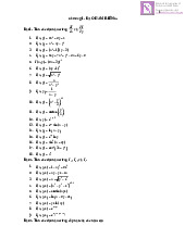
13. f (x) = 4 − x, x ∈ [−1, 4) K
14. f (x) = 3x − 5, x ∈ (−2, 1)
(b) Graph R(N) as a function of N for N ≥ 0 when r = 2 and
15. f (x) = x2 − 2, x ∈ [−1, 1]
K = 100, and find the population size for which the reproductive rate is maximal.
16. f (x) = (x − 2)2, x ∈ [0, 3]
17. f (x) = x ln x, x ∈ [1, 5] 5.1.3
18. f (x) = x2 − x, x ∈ [0, 1]
35. Suppose f (x) = x3, x ∈ [0, 1].
In Problems 19–26, find c such that f (c) = 0 and determine
(a) Find the slope of the secant line connecting the points
whether f (x) has a local extremum at x = c.
(x, y) = (0, 0) and (1, 1).
19. f (x) = x2
20. f (x) = (x − 4)2
(b) Find a number c ∈ (0, 1) such that f (c) is equal to the slope
21. f (x) = −x2
22. f (x) = e−x2
of the secant line you computed in (a), and explain why such a number must exist in (0, 1).
23. f (x) = x3
24. f (x) = ex3
36. Suppose f (x) 25. f (x)
= ex, x ∈ [0, 1]. = (x + 1)2
26. f (x) = (x + 1)3
(a) Find the slope of the secant line connecting the points
27. Show that f (x) = |x| has a local minimum at x = 0 but f (x) (x, y)
is not differentiable at x = (0, 1) and (1, e). = 0.
(b) Find a number c
28. Show that f (x)
∈ (0, 1) such that f (c) is equal to the slope
= |x − 1| has a local minimum at x = 1 but
of the secant line you computed in (a), and explain why such a
f (x) is not differentiable at x = 1. number must exist in (0, 1).
29. Show that f (x) = −|x2 − 4| has local maxima at x = 2 and
37. Suppose that f (x) , 1]. x
= x2, x ∈ [−1
= −2 but f (x) is not differentiable at x = 2 or x = −2.
(a) Find the slope of the secant line connecting the points
30. Show that f (x) = |x2 − 1| has local minima at x = 1 and
(x, y) = (−1, 1) and (1, 1).
x = −1 but f (x) is not differentiable at x = 1 or x = −1.
(b) Find a number c ∈ (−1, 1) such that f (c) is equal to the slope 31. Graph
of the secant line you computed in (a), and explain why such a
f (x) = (1 − |x|)2, −1 ≤ x ≤ 2
number must exist in (−1, 1).
38. Suppose that f (x) = ln x, x ∈ [1, e].
and determine all local and global extrema on [−1, 2].
(a) Find the slope of the secant line connecting the points 32. Graph
(x, y) = (1, 0) and (e, 1).
f (x) = (|x| − 2)3, −3 ≤ x ≤ 3
(b) Find a number c ∈ (1, e) such that f (c) is equal to the slope
of the secant line you computed in (a), and explain why such a
and determine all local and global extrema on [−3, 3].
number must exist in (1, e).
33. Population Growth Suppose the size of a population at time t
39. Suppose that f (x)
is N(t) and its growth rate is given by the logistic growth model
= −x2 + 2. Explain why there exists a
point c in the interval (−1, 2) such that f (c) = −1. dN N
40. Suppose that f (x) c = rN 1 − , t ≥ 0
= x3. Explain why there exists a point in dt K
the interval (−1, 1) such that f (c) = 1.
where r and K are positive constants.
41. Suppose that f (x) = x(2 − x). Explain why there exists a
point c in the interval (0, 2) such that f (c) = 0.
(a) Graph the growth rate of the population dN as a function of dt
population size, N, assuming that r
42. Suppose that f (x)
= 2 and K = 100, and find
= x4(5 − x). Explain why there exists a
the population size for which the growth rate is maximal.
point c in the interval (0, 5) such that f (c) = 0.
(b) Show that whatever the value of the parameters ]. N and K,
43. Suppose that f (x) = x2, x ∈ [a, b
f (N) = rN(1 − N/K), N ≥ 0, is differentiable for N > 0, and
(a) Compute the slope of the secant line through the points
compute f (N).
(a, f (a)) and (b, f (b)).
224 Chapter 5 Applications of Differentiation
(b) Find the point c ∈ (a, b) such that the slope of the tangent
MVT why the total distance that Prof. Roper and Molly travel is
line to the graph of f at (c, f (c)) is equal to the slope of the se-
somewhere between 1.5 miles and 12 miles.
cant line determined in (a). How do you know that such a point
51. Denote the size of a population at time t by N(t), and assume
exists? Show that c is the midpoint of the interval (a, b); that is,
that N(0) = 50 and |dN/dt| ≤ 20 for all t ∈ [0, 5]. What can you
show that c = (a + b)/2.
say about N(5)? [Hint: Remember also that it is impossible for
44. Assume that f is continuous on [a, b] and differentiable on
the number of organisms to become negative].
(a, b). Show that if f (a) < f (b), then f is positive at some point
52. Denote the total biomass in a given area of soil at time t by between a and b.
B(t), and assume that B(0) = 3 and |dB/dt| ≤ 1 for all t ∈ [0, 3].
45. Assume that f is continuous on [a, b] and differentiable on
What can you say about B(3)?
(a, b). Show that if f (x) > 0 for all x ∈ (a, b), then f (a) < f (b).
53. Suppose that f is differentiable for all x ∈ R and, further-
46. Assume that f is continuous on [0, 1] and differentiable on
more, that f satisfies f (0) = 0 and 1 ≤ f (x) ≤ 2 for all x > 0.
(0, 1). Assume that f (1/2) = 0, show by sketching the graph of
(a) Use Corollary 1 of the MVT to show that
a function f (x) that satisfies all of these conditions (you do not
need to write down the equation of the function) that it is not
x ≤ f (x) ≤ 2x
necessary that f (0) = f (1). for all x ≥ 0.
47. A car moves in a straight line. At time t (measured in sec-
(b) Use your result in (a) to explain why f (1) cannot be equal
onds), its position (measured in meters) is to 3. 1
(c) Find an upper and a lower bound for the value of f (1). s(t) =
t2, 0 ≤ t ≤ 10 10
54. Suppose that f is differentiable for all x ∈ R with f (2) = 3
(a) Find its average velocity between t = 0 and t = 10.
and f (x) = 0 for all x ∈ R. Find f (x).
(b) Find its instantaneous velocity for t ∈ (0, 10).
55. Suppose that f (x) = e−|x|, x ∈ [−2, 2].
(c) At what time is the instantaneous velocity of the car equal to
(a) Show that f (−2) = f (2). its average velocity?
(b) Compute f (x), where defined.
48. A car moves in a straight line. At time t (measured in sec-
(c) Show that there is no number c ∈ (−2, 2) such that f (c) = 0.
onds), its position (measured in meters) is
(d) Explain why your results in (a) and (c) do not contradict 1 Rolle’s theorem. s(t) =
t3, 0 ≤ t ≤ 10 100
(e) Use a graphing calculator to sketch the graph of f (x).
(a) Find its average velocity between t = 0 and t = 10.
56. Population Growth In Chapter 4 we learned that
(b) Find its instantaneous velocity for t ∈ (0, 10).
f (x) = erx
(c) At what time is the instantaneous velocity of the car equal to
satisfies the differential equation its average velocity? df
49. Prof. Roper drives to work in stop-and-go traffic. His speed = r f (x)
measured in miles per hour (mph) is given by the following func- dx
tion of time, t, measured in minutes
with f (0) = 1. This exercise will show that f (x) is in fact the only
solution. Suppose that r is a constant and f is a differentiable
v(t ) = 30 + 20 sin(t/5 . ) function satisfying
The total journey time is 1 hour. Explain using the MVT why the
df = rf(x) (5.4)
total distance that he travels in this hour is somewhere between dx 10 and 50 miles.
for all x ∈ R, and f (0) = 1. The following steps will show that
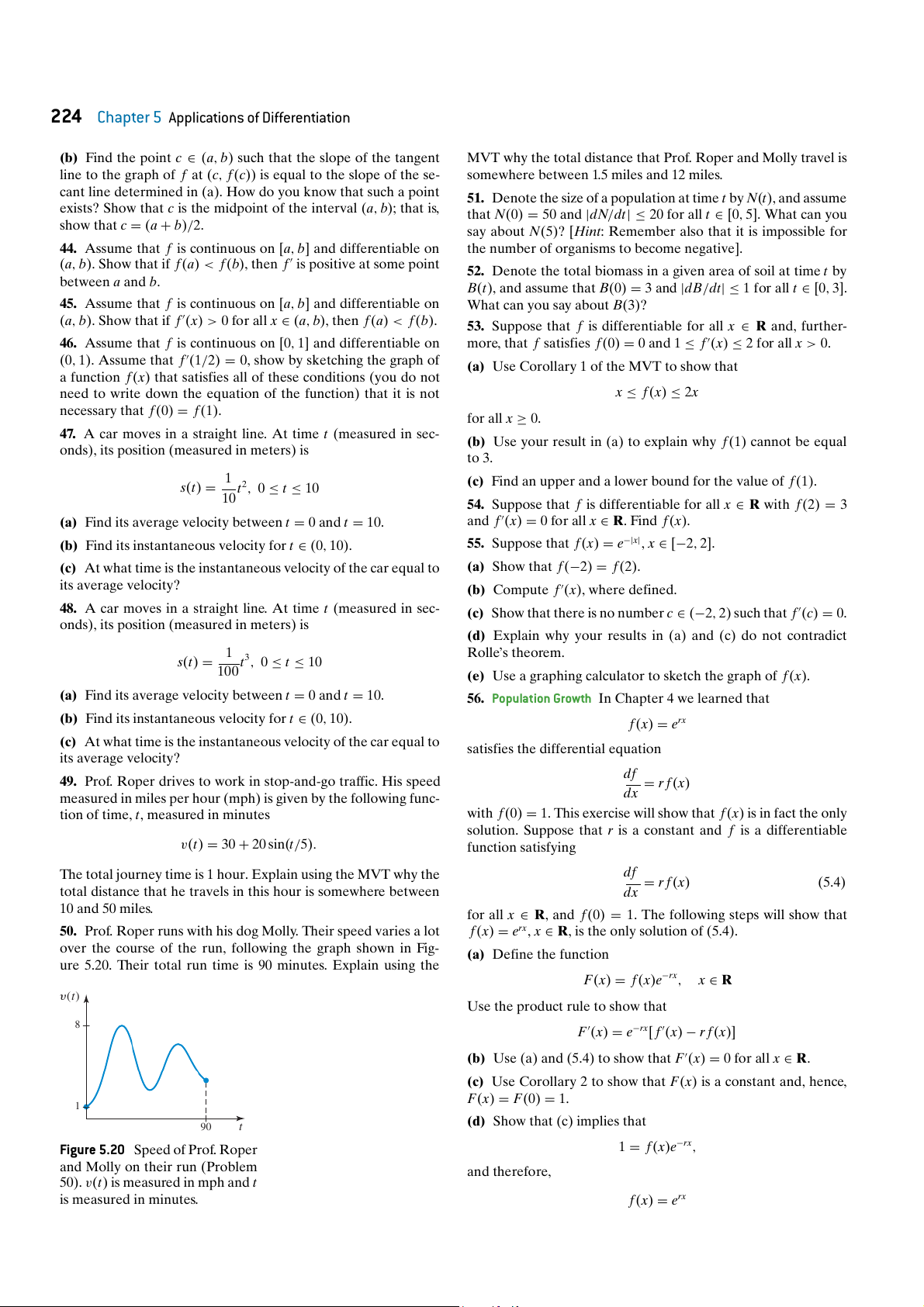
50. Prof. Roper runs with his dog Molly. Their speed varies a lot
f (x) = erx, x ∈ R, is the only solution of (5.4).
over the course of the run, following the graph shown in Fig- (a) Define the function
ure 5.20. Their total run time is 90 minutes. Explain using the
F (x) = f (x)e−rx, x ∈ R y(t)
Use the product rule to show that 8
F (x) = e−rx[ f (x) − r f (x)]
(b) Use (a) and (5.4) to show that F (x) = 0 for all x ∈ R.
(c) Use Corollary 2 to show that F (x) is a constant and, hence,
F (x) = F (0) = 1. 1
(d) Show that (c) implies that 90 t
Figure 5.20 Speed of Prof. Roper
1 = f (x)e−rx,
and Molly on their run (Problem and therefore,
50). v(t) is measured in mph and t is measured in minutes.
f (x) = erx
5.3 Extrema and Inflection Points 241 EXAMPLE 4 Show that the function 1 3
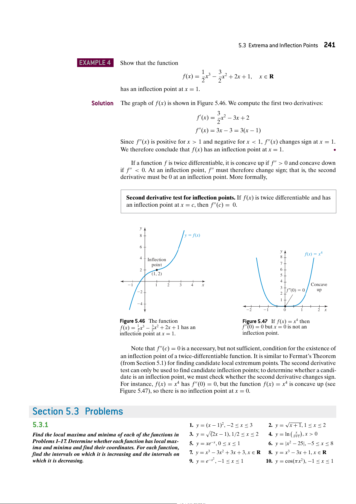
f (x) = x3 − x2 + 2x + 1, x ∈ R 2 2
has an inflection point at x = 1. Solution
The graph of f (x) is shown in Figure 5.46. We compute the first two derivatives: 3
f (x) = x2 − 3x + 2 2
f (x) = 3x − 3 = 3(x − 1)
Since f (x) is positive for x > 1 and negative for x < 1, f (x) changes sign at x = 1.
We therefore conclude that f (x) has an inflection point at x = 1. r
If a function f is twice differentiable, it is concave up if f > 0 and concave down
if f < 0. At an inflection point, f must therefore change sign; that is, the second
derivative must be 0 at an inflection point. More formally,
Second derivative test for inflection points. If f (x) is twice differentiable and has
an inflection point at x = c, then f (c) = 0. y 8 y 5 f (x) 6 y
f (x) 5 x4 4 8 Inflection poin t 7 2 6 (1, 2) 5 4 21 1 2 3 4 x Concave 3 f 0 up 22 (0) 5 0 2 1 24 22 21 0 1 2 x
Figure 5.46 The function
Figure 5.47 If f (x) = x4 then
f (x) = 1 x3
x2 + 2x + 1 has an
f (0) = 0 but x = 0 is not an 2 − 32
inflection point at x = 1. inflection point.
Note that f (c) = 0 is a necessary, but not sufficient, condition for the existence of
an inflection point of a twice-differentiable function. It is similar to Fermat’s Theorem
(from Section 5.1) for finding candidate local extremum points. The second derivative
test can only be used to find candidate inflection points; to determine whether a candi-
date is an inflection point, we must check whether the second derivative changes sign.
For instance, f (x) = x4 has f (0) = 0, but the function f (x) = x4 is concave up (see
Figure 5.47), so there is no inflection point at x = 0. Section 5.3 Problems 5.3.1 √
1. y = (x − 1)2, −2 ≤ x ≤ 3
2. y = x + 1, 1 ≤ x ≤ 2
Find the local maxima and minima of each of the functions in
3. y = (2x − 1), 1/2 ≤ x ≤ 2
4. y = ln x , x > 0 x+1
Problems 1–17. Determine whether each function has local max-
5. y = xe−x, 0 ≤ x ≤ 1
6. y = |x2 − 25|, −5 ≤ x ≤ 8
ima and minima and find their coordinates. For each function,
find the intervals on which it is increasing and the intervals on
7. y = x3 − 3x2 + 3x + 3, x ∈ R
8. y = x3 − 3x + 1, x ∈ R
which it is decreasing.
9. y = e−x2, −1 ≤ x ≤ 1
10. y = cos(πx2), −1 ≤ x ≤ 1
242 Chapter 5 Applications of Differentiation
11. y = e−|x|, x ∈ R
12. y = sin 2πx, 0 ≤ x ≤ 1 (c) Show that
13. y = 1 x3
x2 + 2, x ∈ R lim 3 + 12 N(t) = 100 t→∞
14. y = 1 x3 x 1, x 3 − x2 + + ∈ R
(d) Show that N(t) has an inflection point when N(t) = 50—that
15. y = x2(1 − x), x ∈ R
is, when the size of the population is at half its maximum value. √
16. y = (x − 1)1/3, x ≥ 1
17. y = 1 + x2, x ∈ R
32. Hill’s Function for Hemoglobin Binding Hill’s equation for the
18. [This problem illustrates the fact that f (c) = 0 is not a suffi-
oxygen saturation of blood states that the level of oxygen satura-
cient condition for the existence of a local extremum of a differ-
tion (fraction of hemoglobin molecules that are bound to oxygen)
entiable function.] Show that the function f (x) = x3 has a hor-
in blood can be represented by a function:
izontal tangent at x = 0; that is, show that f (0) = 0, but f (x) Pn f (P)
does not change sign at x =
= 0 and, hence, f (x) does not have a Pn + 30n
local extremum at x = 0.
where P is the oxygen concentration around the blood (P ≥ 0)
19. Explain the first-derivative criterion for local extrema lo-
and n is a parameter that varies between different species.
cated at the right endpoint of the domain of a function. That is, if
(a) Assume that n = 1. Show that f (P) is an increasing function
f (x) is defined on a domain [a, b], and is differentiable on some
of P and that f (P) → 1 as P → ∞.
interval containing x = b, show that x = b is a local maximum
point if f (b) > 0 and a local minimum point if f (b) < 0.
(b) Assuming that n = 1 show that f (P) has no inflection points.
Is it concave up or concave down everywhere?
20. Suppose that f (x) is differentiable on R, with f (x) > 0 for
x ∈ R. Show that if f (x) has a local maximum at x = c, then
(c) Knowing that f (P) has no inflection points, could you deduce
g(x) = ln f (x) also has a local maximum at x = c.
which way the curve bends (whether it is concave up or concave
down) without calculating f (P)?
21. Suppose that f (x) is differentiable on R. Show that if f (x)
has a local maximum at x = c, then g(x) = ef(x) also has a local
(d) For most mammals n is close to 3. Assuming that n = 3 show
maximum at x = c.
that f (P) is an increasing function of P and that f (P) → 1 as P → ∞. 5.3.2
(e) Assuming that n = 3, show that f (P) has an inflection point,
In Problems 22–27, determine all inflection points.
and that it goes from concave up to concave down at this inflec- tion point.
22. f (x) = x3 − 2, x ∈ R
23. f (x) = (x − 3)5, x ∈ R
(f) Using a graphing calculator plot f (P) for n = 1 and n = 3.
24. f (x) = e−x2, x ≥ 0
25. f (x) = xe−x, x ≥ 0
How do the two curves look different?
26. f (x) = x , x ≥ 0
27. f (x) = x2 x+1 x2+1
33. Drug Absorption A two-compartment model of how drugs are π π
absorbed into the body predicts that the amount of drug in the
28. f (x) = tan x, − < x < 2 2
blood will vary with time according to the following function:
29. f (x) = x ln x, x > 0
M(t) = a(e−kt − e−3kt), t ≥ 0
30. [This problem illustrates the fact that f (c) = 0 is not a suf-
where a > 0 and k > 0 are parameters that vary depending on
ficient condition for an inflection point of a twice-differentiable
the patient and the type of drug being administered. For parts
function.] Show that the function f (x) = x4 has f (0) = 0 but
(a)–(c) of this question you should assume that a = 1.
that f (x) does not change sign at x = 0 and, hence, f (x) does
not have an inflection point at x = 0.
(a) Show that M(t) → 0 as t → ∞.
31. Logistic Equation Suppose that the size of a population at
(b) Show that the function M(t) has a single local maximum, and
time t is denoted by N(t) and satisf ies
find the maximum concentration of drug in the patient’s blood. 100
(c) Show that the M(t) has a single inflection point (which you
N(t) = 1 + 3e−2t
should find). Does the function go from concave up to concave for t ≥ 0.
down at this inflection point or vice versa?
(a) Show that N(0) = 25.
(d) Would any of your answers to (a)–(c) be changed if a were
(b) Show that N(t) is strictly increasing. not equal to 1. Which answers? 5.4 Optimization
In Sections 5.1 and 5.3 we showed how calculus can be used to find the extrema of
functions. Calculating extrema is often useful: For example if the function represents
how the crop yield in a field depends on the amount of fertilizer that is added, then
the global maximum of the function tells us how much fertilizer needs to be added to
maximize yields. These kinds of problems are called optimization problems: by maxi-
mizing the yield function we find the optimal amount of fertilizer to add. Optimization
can be used to design experiments of treatments, for example, by predicting the opti-
mal amount of drug to give to a patient. Optimization can also be used to understand 5.5 L’Hˆ opital’s Rule 253
(d) Show that when x = ˆx, the right-hand side of Equation (5.18)
transport and maintenance, show that the xylem vessel radii are can be simplified so that:
related by Murray’s law for plants: d2 w f ( ˆx) R2 = R = r21 + r22 dx2 x ˆ =ˆ x x
29. Evaluating Different Maintenance Cost Functions in Murray’s
So for any function f (x) that is concave down at ˆx, w( ˆx) < 0,
Law When we derived Murray’s law in Examples 4 and 5, we as-
which means that w(x) has a local maximum at ˆx.
sumed that the cost of building and maintaining a blood vessel
28. Murray’s Law for Plants This problem is based on McCulloh et
is proportional to the volume of the vessel (that is, we defined a
al. (2003). The plant xylem is a transport network within plants
quantity b, to be the cost of building and maintaining 1 cm3 of
that forms a network like the blood vessels of animals. The xylem
blood vessel). But this is not the only possibility. Another possi-
transports water from the roots, up the plant stem to its leaves.
bility is that the cost of building a vessel will be proportional to
Unlike blood vessels, in some plants the xylem vessels are not
its surface area, and not to its volume. The idea here is that a wall
single tubes, but are made up of bundles of smaller tubes. Larger
needs to be built around the vessel, and the cost of building the
xylem vessels contain more tubes, smaller vessels contain fewer
vessel wall is much higher than the cost of filling it with blood.
tubes. Because vessels are made of smaller tubes, the way that
Under this assumption, the cost of building and maintaining a
transport costs depend on vessel radius is different for the xylem
vessel of radius r and length is:
than for the blood vessels of an animal. Specifically, it can be
M(r) = 2πcr
shown that the cost of transporting water at a flow rate f (mea-
sured in milliliters/s) in a xylem vessel of radius r and length
where c is the cost of maintaining a 1 cm2 area of vessel wall.
(both measured in cm) is given by the function
(Hint: 2π r is the surface area, not including end-caps for a cylin- f 2
der of length and radius r.)
T (r) = 0.071 r2 r2
(a) Using the same function for the cost of transport within the T where r
vessel as was given in Example 4:
T is the radius of one of the tubes within the xylem vessel
(you may assume that rT = 5 × 10⁻² cm). f 2 T (r) = 0.071
(a) Assume that the cost of building the xylem vessel is still pro- r4 portional to its volume:
and assuming that the organism controls vessel radius to min-
M(r) = bπr2
imize the total cost of transport and maintenance T (r) + M(r),
where b is the metabolic cost of building and maintaining 1 cm3
derive a formula relating blood vessel radius r to flow rate f . Your
of xylem vessel. If the plant controls xylem vessel radius to min-
formula will include c as an unknown coefficient.
imize the total cost T (r) + M(r), derive a formula relating xylem
(b) If a blood vessel of radius R branches into two smaller ves-
radius r to flow rate f . Your formula will include b as an unknown
sels of radii r1 and r2, and all vessels minimize the total cost of coefficient.
transport and maintenance, show that the blood vessel radii are
related by a modified form of Murray’s law:
(b) If a xylem vessel of radius R branches into two smaller ves- sels of radii r / /
1 and r2, and all vessels minimize the total cost of R5/2 = r5 2 1 + r5 2 2 5.5 L’Hˆopital’s Rule
L’H ˆopital’s rule gives us a way to calculate the limits of fractions in which both the
numerator and the denominator tend to 0. (l’H ˆopital is pronounced lop-it-al.) The rule
also works when both the numerator and the denominator tend to infinity. Sometimes
we can use algebraic or trigonometric manipulations to find the limit—for instance: x2 − 9 lim = lim (x + 3) = 6
Factorize x2 − 9 = (x + 3)(x − 3) and cancel (x − 3) x→3 x − 3 x→3 x 1 lim = lim = 1
Divide numerator and denominator by x y x→∞ 1
f (x) 5 ex 2 1 + x x→∞ 1 + 1 x 2
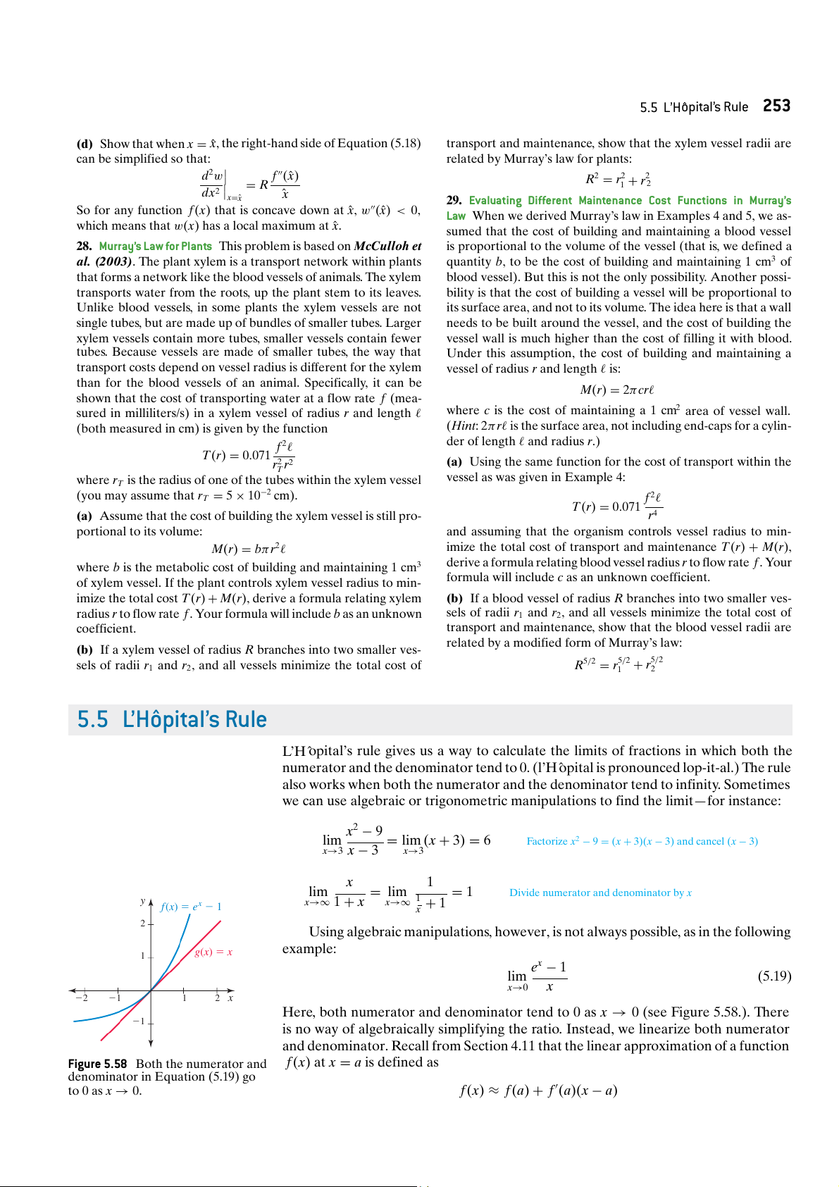
Using algebraic manipulations, however, is not always possible, as in the following g(x) 5 x example: 1 ex − 1 lim (5.19) x→0 x 2 2 2 1 1 2 x
Here, both numerator and denominator tend to 0 as x → 0 (see Figure 5.58.). There 21
is no way of algebraically simplifying the ratio. Instead, we linearize both numerator
and denominator. Recall from Section 4.11 that the linear approximation of a function
Figure 5.58 Both the numerator and
f (x) at x = a is defined as
denominator in Equation (5.19) go to 0 as x → 0.
f (x) ≈ f (a) + f (a)(x − a)
254 Chapter 5 Applications of Differentiation y
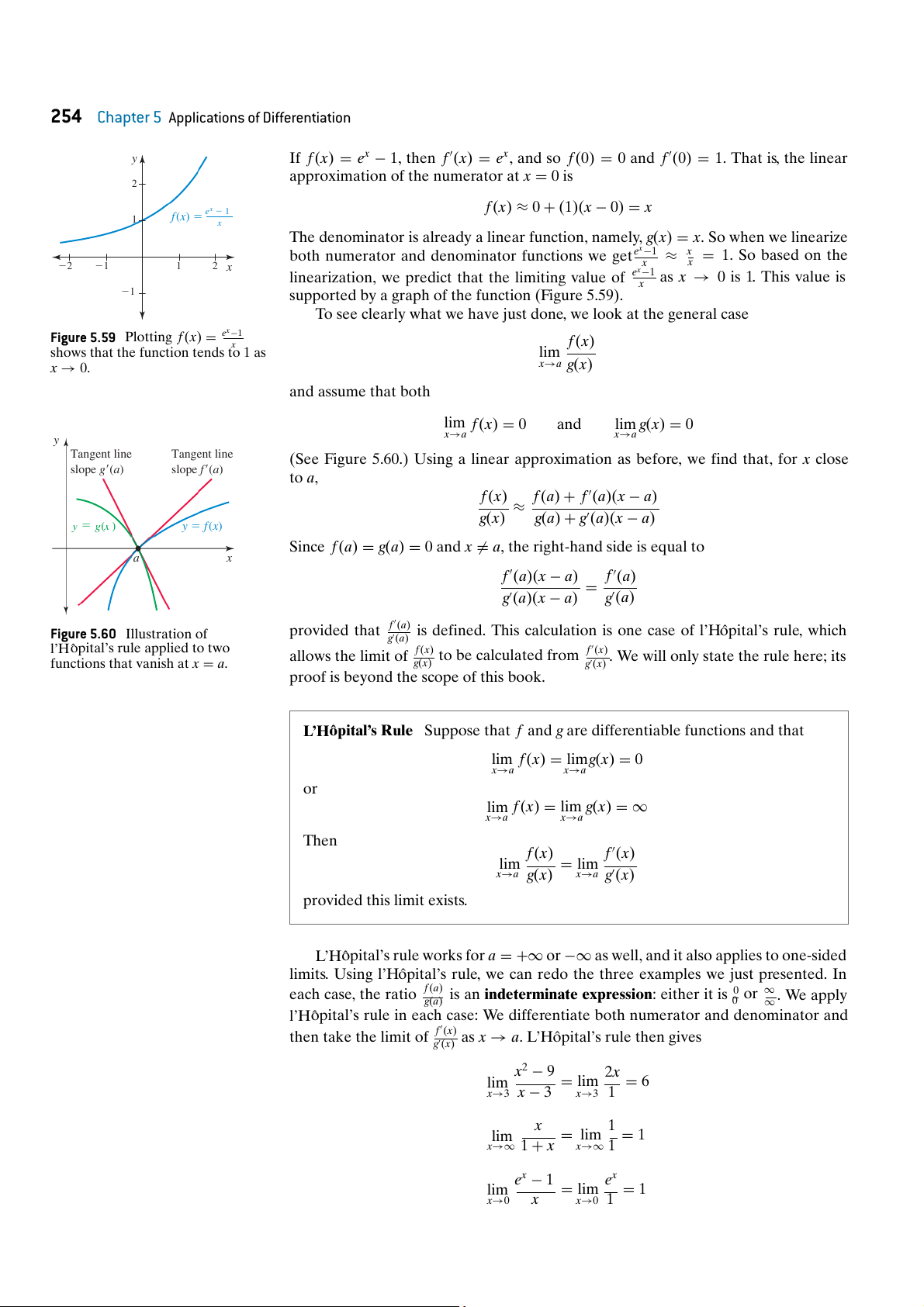
If f (x) = ex − 1, then f (x) = ex, and so f (0) = 0 and f (0) = 1. That is, the linear
approximation of the numerator at x = 0 is 2 ex 2 1
f (x) ≈ 0 + (1)(x − 0) = x 1 f (x) 5 x
The denominator is already a linear function, namely, g(x) = x. So when we linearize
both numerator and denominator functions we getex−1 ≈ x = 1. So based on the 2 2 x x 2 1 1 2 x
linearization, we predict that the limiting value of ex−1 as x → 0 is 1. This value is x 21
supported by a graph of the function (Figure 5.59).
To see clearly what we have just done, we look at the general case
Figure 5.59 Plotting f (x) = ex−1 x f (x)
shows that the function tends to 1 as lim x → 0.
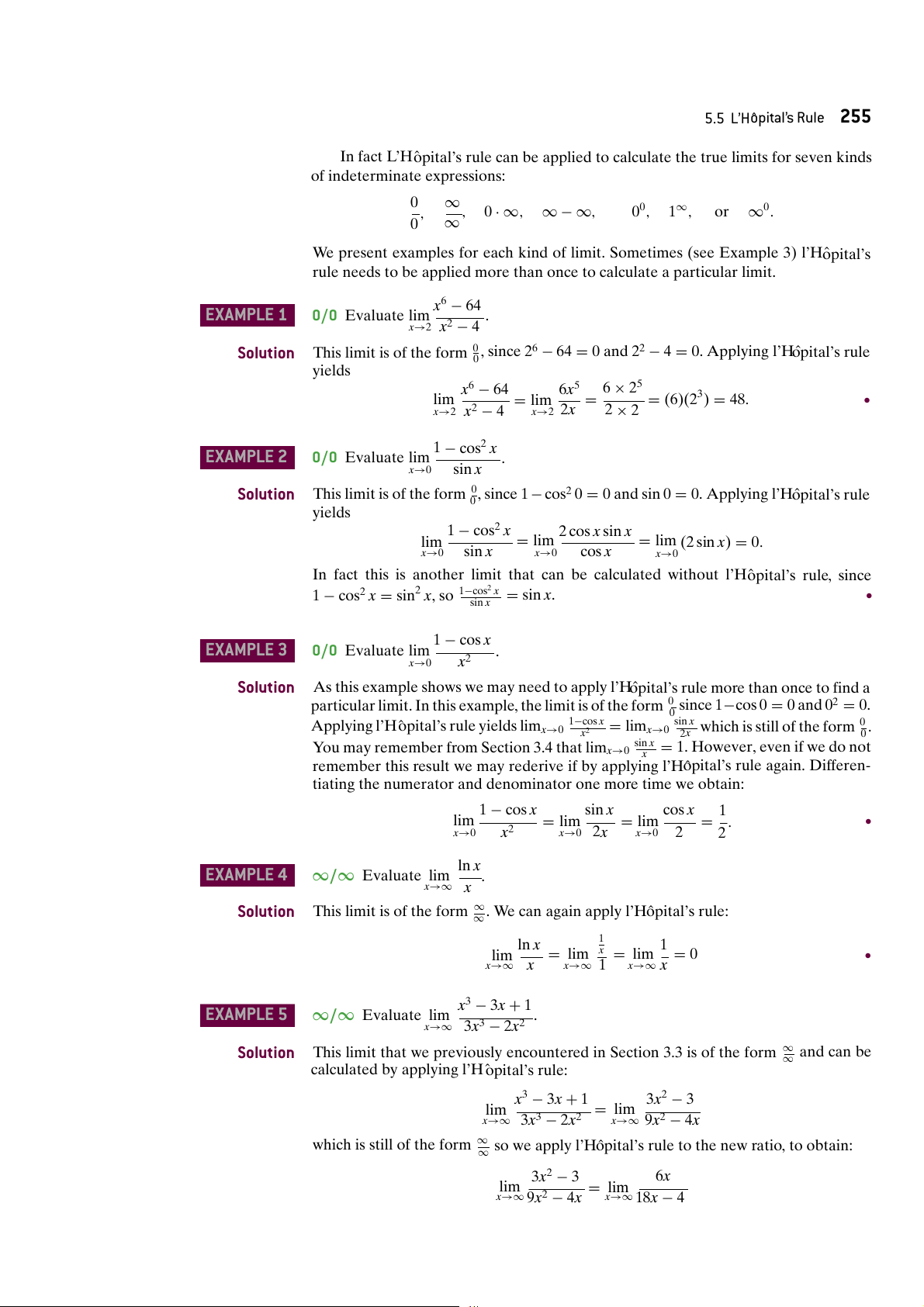
x→a g(x) and assume that both lim f (x) = 0 and lim g(x) = 0 y x→a x→a Tangent line Tangent line
(See Figure 5.60.) Using a linear approximation as before, we find that, for x close slope g9(a) slope f9(a) to a, f (x)
f (a) + f (a)(x − a) ≈ g(x) g(a) y 5 g
+ g(a)(x − a) (x ) y 5 f (x)
Since f (a) = g(a) = 0 and x = a, the right-hand side is equal to a x
f (a)(x − a) f (a) =
g(a)(x − a) g(a) a
Figure 5.60 Illustration of
provided that f( ) is defined. This calculation is one case of l’H ˆopital’s rule, which g(a)
l’H ˆopital’s rule applied to two
allows the limit of f(x) to be calculated from f(x). We will only state the rule here; its
functions that vanish at x = a. g(x) g(x)
proof is beyond the scope of this book.
L’H ˆopital’s Rule Suppose that f and g are differentiable functions and that
lim f (x) = limg(x) = 0 x→a x→a or
lim f (x) = lim g(x) = ∞ x→a x→a Then f (x) f (x) lim = lim
x→a g(x)
x→a g(x) provided this limit exists.
L’H ˆopital’s rule works for a = +∞ or −∞ as well, and it also applies to one-sided
limits. Using l’H ˆopital’s rule, we can redo the three examples we just presented. In
each case, the ratio f(a) is an indeterminate expression: either it is 0 or ∞ . We apply g(a) 0 ∞
l’H ˆopital’s rule in each case: We differentiate both numerator and denominator and
then take the limit of f(x) as x → a. L’H ˆopital’s rule then gives g(x) x2 − 9 2x lim = lim = 6 x→3 x − 3 x→3 1 x 1 lim = lim = 1 x→∞ 1 + x x→∞ 1 ex − 1 ex lim = lim = 1 x→0 x x→0 1 5.5 L’Hˆ opital’s Rule 255
In fact L’H ˆopital’s rule can be applied to calculate the true limits for seven kinds of indeterminate expressions: 0 ∞ , , 0 · ∞, ∞ − ∞, 00, 1∞, or ∞0. 0 ∞
We present examples for each kind of limit. Sometimes (see Example 3) l’H ˆopital’s
rule needs to be applied more than once to calculate a particular limit. EXAMPLE 1 x6 − 64 0/0 Evaluate lim . x→2 x2 − 4 Solution
This limit is of the form 0 , since 26 0
− 64 = 0 and 22 − 4 = 0. Applying l’H ˆ opital’s rule yields x6 − 64 6x5 6 × 25 lim = lim = = (6)(23) = 48. r x→2 x2 − 4 x→2 2x 2 × 2 EXAMPLE 2 1 − cos2 x 0/0 Evaluate lim . x→0 sin x Solution
This limit is of the form 0, since 1 0 and sin 0
0. Applying l’H ˆopital’s rule 0 − cos2 0 = = yields 1 − cos2 x 2 cos x sin x lim = lim = lim (2 sin x) = 0. x→0 sin x x→0 cos x x→0
In fact this is another limit that can be calculated without l’H ˆopital’s rule, since
1 − cos2 x = sin2 x, so 1−cos2 x sin = sin x. r x 1 EXAMPLE 3 − cos x 0/0 Evaluate lim . x→0 x2 Solution
As this example shows we may need to apply l’Hˆ
opital’s rule more than once to find a
particular limit. In this example, the limit is of the form 0 since 1 0 −cos 0 = 0 and 02 = 0.
Applying l’H ˆopital’s rule yields lim 1−cos x sin x x→0 which is still of the form 0 . x2 = limx→0 2x 0
You may remember from Section 3.4 that lim sin x x→0
= 1. However, even if we do not x
remember this result we may rederive if by applying l’H ˆopital’s rule again. Differen-
tiating the numerator and denominator one more time we obtain: 1 − cos x sin x cos x 1 lim = lim = lim = . r x→0 x2 x→0 2x x→0 2 2 ln x EXAMPLE 4 ∞/∞ Evaluate lim . x→∞ x Solution
This limit is of the form ∞. We can again apply l’H ˆopital’s rule: ∞ ln x 1 1 lim = lim x = lim = 0 r x→∞ x x→∞ 1 x→∞ x EXAMPLE 5 x3 − 3x + 1 ∞/∞ Evaluate lim .
x→∞ 3x3 − 2x2 Solution
This limit that we previously encountered in Section 3.3 is of the form ∞ and can be ∞
calculated by applying l’H ˆopital’s rule: x3 − 3x + 1 3x2 − 3 lim = lim
x→∞ 3x3 − 2x2
x→∞ 9x2 − 4x
which is still of the form ∞ so we apply l’H ˆopital’s rule to the new ratio, to obtain: ∞ 3x2 − 3 6x lim = lim
x→∞ 9x2 − 4x
x→∞ 18x − 4
256 Chapter 5 Applications of Differentiation
Since this is still of the form ∞, we can apply l’H ˆopital’s rule yet again. We now find ∞ that 6x 6 1 lim = lim =
x→∞ 18x − 4 x→∞ 18 3
In fact we could have found the answer without using l’H ˆ
opital’s rule by following the
rules in Section 3.3. Divide both numerator and denominator by x3 to obtain: x3 − 3x + 1 (1 − 3 ) 1 lim = lim x2 + 1 x3 = ,
x→∞ 3x3 − 2x2 x→∞ (3 − 2) 3 x
because terms 3 , 1 , etc., all → 0. r x2 x3 EXAMPLE 6 ex ∞/∞ Evaluate lim . x→∞ x Solution
This limit is of the form ∞ . The example will show that l’H ˆopital’s rule has no problems ∞
detecting when a limit is infinite. ex ex lim = lim = ∞ (limit does not exist) r x→∞ x x→∞ 1
0 · ∞ L’H ˆopital’s rule can sometimes be applied to limits of the form
lim f (x)g(x) x→a where lim f (x) = 0 and lim g(x) = ∞. x→a x→a
To apply l’H ˆopital’s rule to these limits write them in one of the two forms: f (x) g(x)
lim f (x)g(x) = lim = lim . x→a x→a 1 x→a 1 g(x) f (x)
In the first case, the ratio is 0, while in the second case the ratio is ∞ . Usually only 0 ∞
one of the two methods for rewriting the expression actually makes the limit easier to
evaluate, as the following example shows: EXAMPLE 7
0 ·∞ Evaluate limx . →0+ x ln x Solution
This is a one-sided limit, but l’H ˆ
opital’s rule still applies. ln x is not defined for x ≤ 0
so we must approach x = 0 from the right. The limit is of the form (0)(− ) ∞ . We apply
l’H ˆopital’s rule after rewriting it in the form ∞: ∞ ln x 1 lim x ln x = lim = lim x x→0+ x→0+ 1 x→0+ − 1 x x2 1 x2 = lim − = lim (−x) = 0 x→0+ x 1 x→0+
If we had written the limit in the form x lim x→0+ 1 ln x and then applied l’H ˆ
opital’s rule, we would have obtained x 1 lim = lim
= lim −x(ln x)2 x→0+ 1 x x→0+ ln →0+ ( x
−1)(ln x)−2 1x
which is more complicated than the initial expression. In general you may need to try
both ways of rewriting expressions of the form 0 · ∞ to find an expression you can evaluate. r 5.5 L’Hˆ opital’s Rule 257 EXAMPLE 8
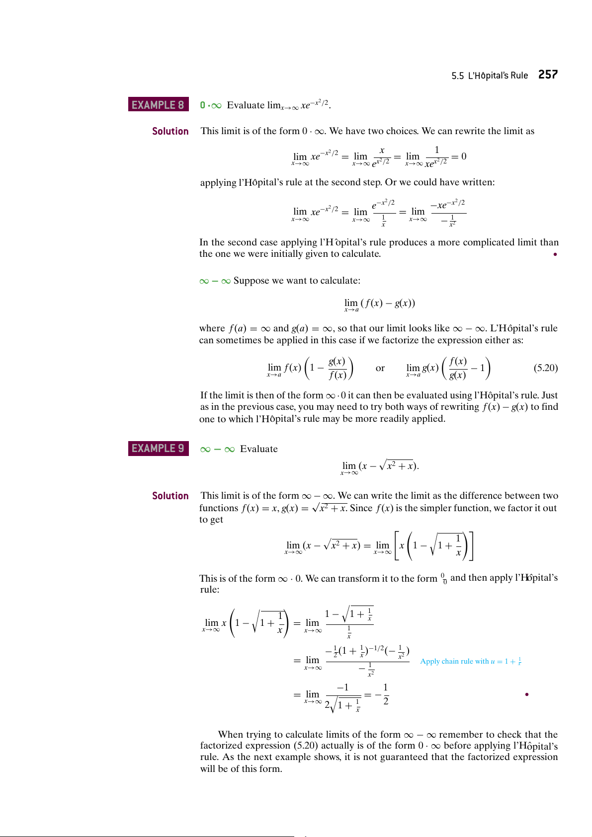
0 ·∞ Evaluate limx→∞ xe−x2/2. Solution
This limit is of the form 0 · ∞. We have two choices. We can rewrite the limit as x 1
lim xe−x2/2 = lim = lim = 0 x→∞ x→∞ ex2/2 x→∞ xex2/2
applying l’H ˆopital’s rule at the second step. Or we could have written: e−x2/2 −xe−x2/2
lim xe−x2/2 = lim = lim x→∞ x→∞ 1 x→∞ x − 1x2
In the second case applying l’H ˆopital’s rule produces a more complicated limit than
the one we were initially given to calculate. r
∞ − ∞ Suppose we want to calculate:
lim ( f (x) − g(x)) x→a
where f (a) = ∞ and g(a) = ∞, so that our limit looks like ∞ − ∞. L’H ˆopital’s rule
can sometimes be applied in this case if we factorize the expression either as: g(x) f (x) lim f (x) 1 − or lim g(x) − 1 (5.20) x→a f (x) x→a g(x)
If the limit is then of the form ∞ · 0 it can then be evaluated using l’H ˆopital’s rule. Just
as in the previous case, you may need to try both ways of rewriting f (x) − g(x) to find
one to which l’H ˆopital’s rule may be more readily applied. EXAMPLE 9 ∞ − ∞ Evaluate
lim (x − x2 + x). x→∞ Solution
This limit is of the form ∞ − ∞. We can write the limit as the difference between two √
functions f (x) = x, g(x) = x2 + x. Since f (x) is the simpler function, we factor it out to get 1
lim (x − x2 + x) = lim x 1 − 1 + x→∞ x→∞ x
This is of the form ∞ · 0. We can transform it to the form 0 and then apply l’H ˆ opital’s 0 rule: 1 1 − 1 + 1 lim x 1 x − 1 + = lim x→∞ x x→∞ 1 x − 1 (1 )−1/2( ) 2 + 1x − 1 = lim x2
Apply chain rule with u = 1 + 1x x→∞ − 1x2 −1 1 = lim = − r x→∞ 2 1 + 1 2 x
When trying to calculate limits of the form ∞ − ∞ remember to check that the
factorized expression (5.20) actually is of the form 0 · ∞ before applying l’H ˆopital’s
rule. As the next example shows, it is not guaranteed that the factorized expression will be of this form.
258 Chapter 5 Applications of Differentiation EXAMPLE 10
∞ − ∞ Evaluate limx→+∞ (x − ln x). Solution
Our limit takes the form of the difference between the functions f (x) = x and g(x) =
ln x. Since x is the simpler function we factorize it out to obtain: ln x
lim (x − ln x) = lim x 1 − x→+∞ x→+∞ x
The first factor has limit ∞. However, the limit of the second factor is actually 1, since: ln x ln x lim 1 − = 1 − lim = 1 − 0 = 1 lim ln x x→+∞ x x x = 0, from Example 4 →+∞ x x→∞
So the product of the two factors has a limit of the form ∞·1. The limit is therefore ∞ or undefined.
00, 1∞, ∞0 Suppose we want to evaluate
lim [ f (x)]g(x) x→a
when ( f (a), g(a)) = (0, 0), (1, ∞), or (∞, 0). The key to solving such limits is to rewrite them as exponentials:
lim [ f (x)]g(x) = lim exp ln [ f (x)]g(x) x→a x→a y
= lim exp [g(x) · ln f (x)] x→a 3
= exp lim (g(x) · ln f (x)) x→a y 5 x x 2
The last step, in which we interchanged lim and exp, uses the fact that the exponential
function is continuous. Rewriting the limit in this way transforms 1 00 into exp [0 · (−∞)] ∞0 into exp [0 · ∞] 0 0 1 2 x 1∞ into
exp [∞ · ln 1] = exp [∞ · 0]
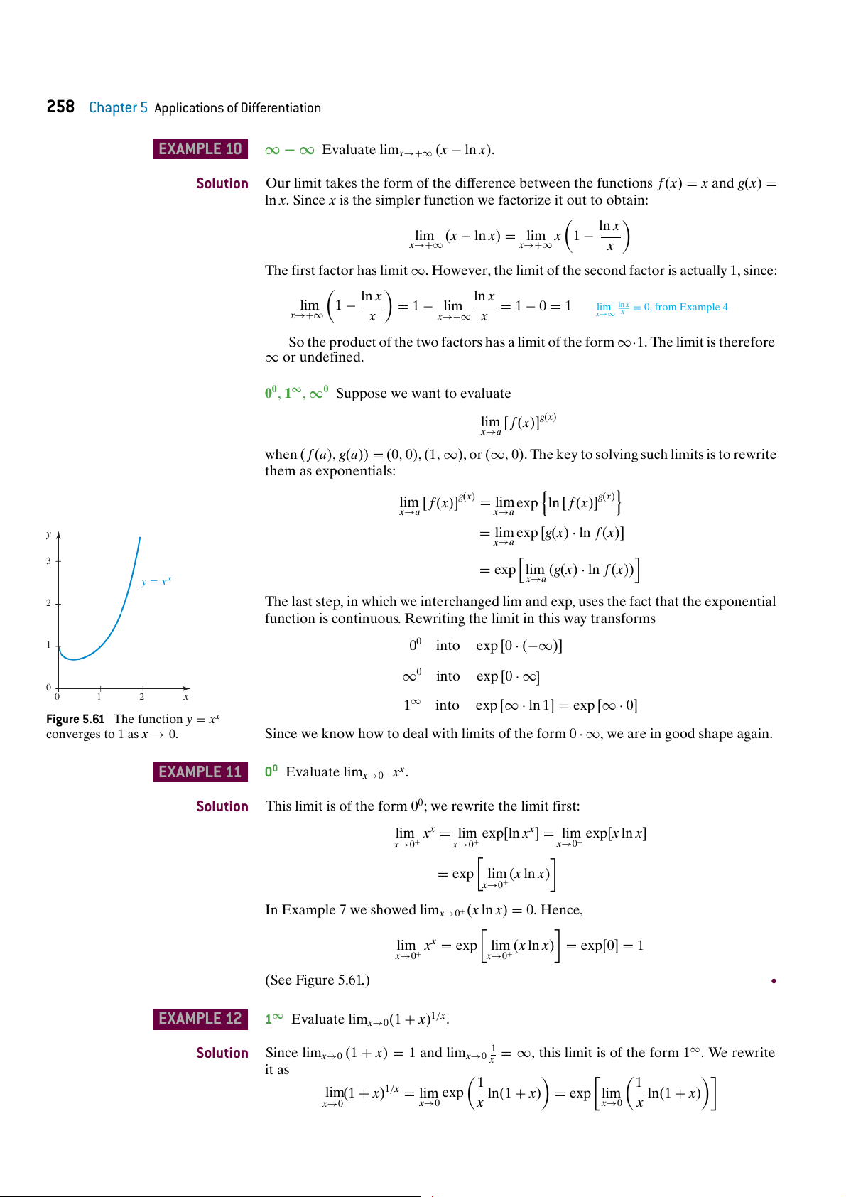
Figure 5.61 The function y = xx
converges to 1 as x → 0.
Since we know how to deal with limits of the form 0 · ∞, we are in good shape again. EXAMPLE 11
00 Evaluate limx→0+ xx. Solution
This limit is of the form 00; we rewrite the limit first:
lim xx = lim exp[ln xx] = lim exp[x ln x] x→0+ x→0+ x→0+
= exp lim (x ln x) x→0+
In Example 7 we showed limx→0+(x ln x) = 0. Hence,
lim xx = exp lim (x ln x) = exp[0] = 1 x→0+ x→0+ (See Figure 5.61.) r EXAMPLE 12 1∞ Evaluate lim 1/x x→0(1 + x) . Solution Since lim 1
x→0 (1 + x) = 1 and limx→0
= ∞, this limit is of the form 1∞. We rewrite x it as 1 1
lim(1 + x)1/x = lim exp ln(1 + x) = exp lim ln(1 + x) x→0 x→0 x x→0 x 5.5 L’Hˆ opital’s Rule 259
The exponentiated function is of the form ∞ · 0 (since ln 1 = 0). We evaluate the limit
of this function by writing it in the form 0 and then applying l’H ˆopital’s rule: 0 ln(1 1 + x) lim = lim 1+x = 1. x→0 x x→0 1
Therefore, limx→0(1 + x)1/x = exp(1) = e. r Section 5.5 Problems √
Find the limits in Problems 1–60; not all limits require use of 1 1
x2 + x4 − x 39. lim 40. lim
l’H ˆopital’s rule. − x→0+ sin x x x→0 x x2 − 25 x − 2 1. lim 2. lim
41. lim x2x 42. lim xx2 x x →5 x − 5 x→2 x2 − 4 x→0+ →0+ 3x2 + 5x − 2 x + 1
43. lim x1/x
44. lim (1 + ex)1/x 3. lim 4. lim x→∞ x→∞ x→−2 x + 2
x→−1 x2 − 2x − 3 3x 5x √ √ 45. lim 1 + 46. lim 1 + 3 − 2x + 9 2x + 4 − 2 x→∞ x x→∞ x 5. lim 6. lim x x x→0 2x x→0 x 2 3 47. lim 1 − 48. lim 1 + ln x x→∞ x x→∞ x2
7. lim x2 ln x 8. lim x→0 x→∞ x2 x x √ √ √ 49. lim
50. lim (1 + x)1/x
9. lim ln x − x 10. lim x − x + 3 x→∞ 1 + x x→∞ x→∞ x→∞ √ ex x ln x 51. lim xex 52. lim 11. lim 12. lim √ x→0 x→0+ x x→0+ ln(x + 1) x→∞ x 1 sin x
53. lim (ln(1 − x) − ) 54. lim ln(ln x) ln(ln x) x→1− x − 1
x→(π/2)− cos x 13. lim 14. lim x→∞ x x→∞ ln x x2 − 1 1 − cos x 55. lim 56. lim 5x − 1 2x − 1 x→1 x + 1 x→0 x 15. lim 16. lim x→0 7x − 1 x→0 3x − 1 1 1 57. lim xex 58. lim − √ x→−∞ x x 3−x x − 1 2−x − 1 →0+ 17. lim 18. lim √x x x x→0 2x − 1 x→0 5x − 1 + 1 + 1 59. lim √ 60. lim x→+∞ x x→∞ x + 2 ex − 1 − x ex − 1 19. lim 20. lim
61. Use l’H ˆopital’s rule to find x→∞ ex − x2
x→0 3e2x − x ax − 1 (ln x)2 x7 lim 21. lim 22. lim x→0 bx − 1 x→∞ x2 x→∞ ex
where a, b > 0. sin x sin x 23. lim 24. lim
62. Use l’H ˆopital’s rule to find x→0 x x→0 x2 c x lim 1 +
25. lim xe−x
26. lim x2e−x x→∞ x x→∞ x→∞ where c is a constant.
27. lim x5e−x
28. lim xne−x, n ∈ N
63. For p > 0, determine the values of p for which the following x→∞ x→∞
limit is either 1 or ∞ or a constant that is neither 1 nor ∞: √ 29. lim x ln x
30. lim xα ln x, α > 0 is any x x→0+ x→0+ 1 positive constant lim 1 + x→∞ xp ln x ln x 31. lim 32. lim , α > 0 is any
64. Cell Division Time The Gamma distribution is used as a model x→+∞ x1/2 x→+∞ xα positive constant
for the amount of time taken for a cell to undergo a certain
number of divisions. According to the Gamma distribution the
33. lim ex − x3
34. lim (ex − xn), n ∈ N
likelihood that it takes t hours for the cell to complete all of its x→+∞ x→+∞ divisions is proportional to: √ 1 1 35. lim x sin 36. lim x2 sin
f (t) = t pe−t x→∞ x x→∞ x2
where p > −1 is a constant that depends on the number of 1
37. lim (ex − )
38. lim (x − x2 + 1)
cells that are dividing, and on the conditions that the cells are x→0+ x x→∞ growing in.
260 Chapter 5 Applications of Differentiation
(a) Show that for all values of p, f (t) → 0 as t → ∞.
different species of animals, and they are present in the propor-
(b) For what values of p does f (t) converge to a finite value as
tions p and 1 − p respectively, then the Shannon diversity index t
for the population is given by the formula: → 0?
65. Lifespan Modeling The Weibull distribution is used to model
H(p) = −p ln p − (1 − p) ln(1 − p) , 0 < p < 1
the lifespan of organisms. According to the Weibull distribution,
the likelihood that an animal dies at the age of t is proportional
(a) Show that if H(0) = 0 and H(1) = 0, then the function H(p) to:
is continuous at p = 0 and p = 1. (Hint: This is equivalent to showing that lim = 0 and lim
f (t) = tk−1 exp −tk , t ≥ 0
p→0+ H( p) p )
→1− H( p = 0.)
(b) Show that the global maximum diversity over the interval
where k > 0 is a constant that depends on the type of organism
0 ≤ p ≤ 1 occurs when p = 1/2.
being studied, and on the environment that it is living in.
68. The height y in feet of a tree as a function of the tree’s age x
(a) Show that for all values of k, f (t) → 0 as t → ∞. in years is given by
(b) For what values of k does f (t) converge to a finite value as t → 0?
y = 121e−17/x for x > 0 66. Show that ln x
(a) Determine (1) the rate of growth when x lim → 0+ and (2) the = 0 x→∞ xp
limit of the height as x → ∞.
for any number p > 0. This shows that the logarithmic function
(b) Find the age at which the growth rate is maximal.
grows more slowly than any positive power of x as x → ∞.
(c) Show that the height of the tree is an increasing function of
67. Species Diversity Chapter 3 introduced the Shannon diversity
age. At what age is the height increasing at an accelerating rate
index for the diversity of a habitat. If a population contains two
and at what age at a decelerating rate? 5.6 Graphing and Asymptotes
Calculus tools can be used to draw the graph of a function. Being able to graph a
function may feel like a redundant skill since graphing calculators or spreadsheets can
be used to plot any function. But there are many cases where the function that we y
are interested in has one (or more) unknown constants. For example, some insects 12,000
(e.g., locusts and cicadas) undergo explosive population growth and then decay. One 10,000
possible mathematical model for the population growth and decay is 8000 20.1t 6000
y 5 100t 2e
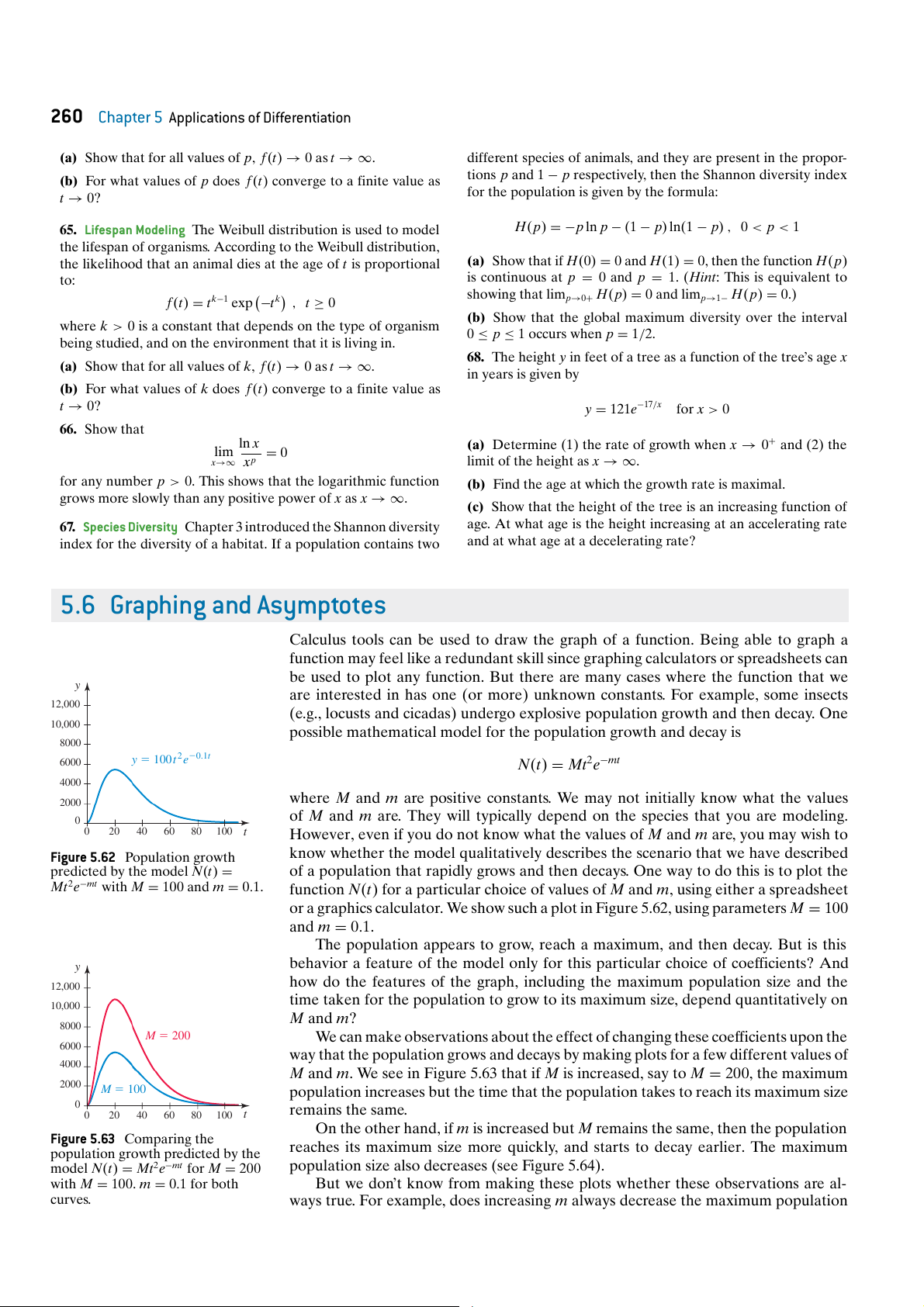
N(t) = Mt2e−mt 4000 2000
where M and m are positive constants. We may not initially know what the values 0
of M and m are. They will typically depend on the species that you are modeling. 0 20 40 60 80 100 t
However, even if you do not know what the values of M and m are, you may wish to
know whether the model qualitatively describes the scenario that we have described
Figure 5.62 Population growth
predicted by the model N(t) =
of a population that rapidly grows and then decays. One way to do this is to plot the
Mt2e−mt with M = 100 and m = 0.1.
function N(t) for a particular choice of values of M and m, using either a spreadsheet
or a graphics calculator. We show such a plot in Figure 5.62, using parameters M = 100 and m = 0.1.
The population appears to grow, reach a maximum, and then decay. But is this y
behavior a feature of the model only for this particular choice of coefficients? And 12,000
how do the features of the graph, including the maximum population size and the
time taken for the population to grow to its maximum size, depend quantitatively on 10,000 M and m? 8000 M 5 200
We can make observations about the effect of changing these coefficients upon the 6000
way that the population grows and decays by making plots for a few different values of 4000
M and m. We see in Figure 5.63 that if M is increased, say to M = 200, the maximum 2000 M 5 100
population increases but the time that the population takes to reach its maximum size 0 0 20 40 60 80 100 t remains the same.
On the other hand, if m is increased but M remains the same, then the population
Figure 5.63 Comparing the
population growth predicted by the
reaches its maximum size more quickly, and starts to decay earlier. The maximum
model N(t) = Mt2e−mt for M = 200
population size also decreases (see Figure 5.64).
with M = 100. m = 0.1 for both
But we don’t know from making these plots whether these observations are al- curves.
ways true. For example, does increasing m always decrease the maximum population
Tài liệu liên quan:
-
Bài tập Toán cao cấp 1 | Trường Đại học Tôn Đức Thắng
49 25 -
Bài tập môn Toán cao cấp 1 | Trường Đại học Tôn Đức Thắng
37 19 -
Bài tập môn Toán cao cấp 1 | Trường Đại học Tôn Đức Thắng
40 20 -
Giới thiệu Đại số tuyến tính môn Toán cao cấp | Trường Đại học Tôn Đức Thắng
41 21 -
Giới Hạn Trong Giải Tích | Toán cao cấp 1 | Đại học Tôn Đức Thắng
167 84