Bài tập ôn tập tuần 8 | Microeconomics | Trường Đại học Quốc tế, Đại học Quốc gia Thành phố Hồ Chí Minh

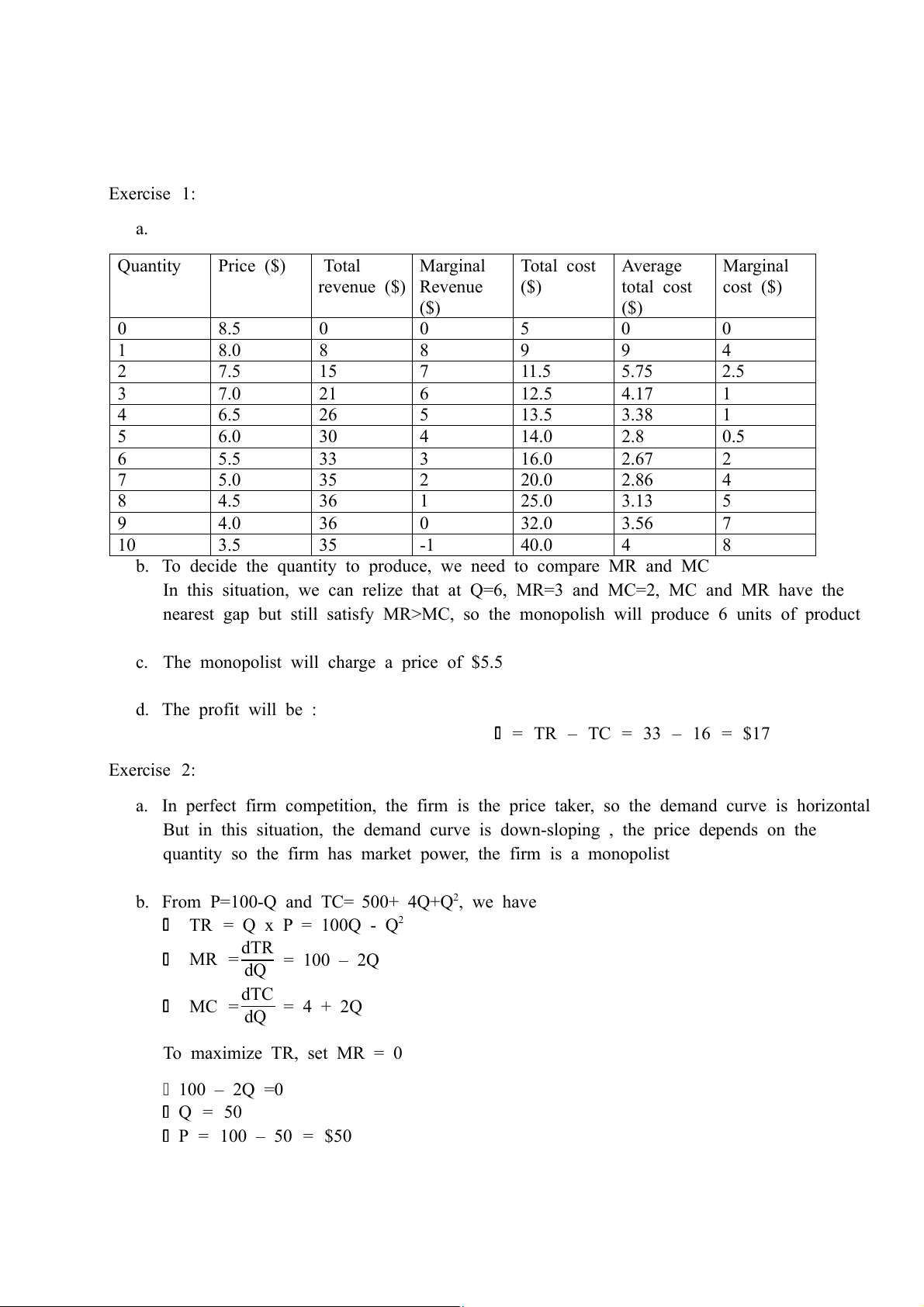
Exercise 1: a. Quantity Price ($) Total Marginal Total cost Average Marginal revenue ($) Revenue ($) total cost cost ($) ($) ($) 0 8.5 0 0 5 0 0 1 8.0 8 8 9 9 4 2 7.5 15 7 11.5 5.75 2.5 3 7.0 21 6 12.5 4.17 1 4 6.5 26 5 13.5 3.38 1 5 6.0 30 4 14.0 2.8 0.5 6 5.5 33 3 16.0 2.67 2 7 5.0 35 2 20.0 2.86 4 8 4.5 36 1 25.0 3.13 5 9 4.0 36 0 32.0 3.56 7 10 3.5 35 -1 40.0 4 8
b. To decide the quantity to produce, we need to compare MR and MC
In this situation, we can relize that at Q=6, MR=3 and MC=2, MC and MR have the
nearest gap but still satisfy MR>MC, so the monopolish will produce 6 units of product
c. The monopolist will charge a price of $5.5 d. The profit will be :
= TR – TC = 33 – 16 = $17 Exercise 2:
a. In perfect firm competition, the firm is the price taker, so the demand curve is horizontal
But in this situation, the demand curve is down-sloping , the price depends on the
quantity so the firm has market power, the firm is a monopolist b. From P=100-Q and TC= 500+ 4Q+Q , 2 we have TR = Q x P = 100Q - Q2 dTR MR = dQ = 100 – 2Q dTC MC = dQ = 4 + 2Q To maximize TR, set MR = 0 100 – 2Q =0 Q = 50
P = 100 – 50 = $50 TR = 100 x 50 - 50 2 = $2500
c. To decide the quantity of product to maximize profit, we find Q* through MR=MC equation
100 – 2Q = 4 + 2Q => Q* = 24
P = 100 -24 = $76
= TR – TC = [(100 x 24) - 24 2 ] - [500+ (4 x 24) +24 ] 2 =$652
d. After tax, the new total cost is
TC =500+ 4Q+Q2+8Q = 500+ 12Q+Q2 MC = 12 + 2Q
To decide the quantity of product to maximize profit, we find Q* through MR=MC equation
100 – 2Q = 12 + 2Q => Q* = 22 P = $ 78
= TR – TC =[(100 x 22) - 22 2 ] - [500+ (12 x 22) +22 ] 2 = $468
e. After fixed tax, only TC increases by $100, MC remains unchanged. Thus, the condition
MR=MC is unchanged from (c), we have Q* = 24, P = $76
But there is a decrease of $100 in the profit because of the fixed tax: = 653–100 = $553 Exercise 3:
a. From P= 15-Q and TC= 7Q, we have: TR = P x Q = 15Q – Q2 dTC MC = =7 dQ dTR MR = dQ = 15 – 2Q
To decide the quantity of product to maximize profit, we find Q* through MR=MC equation:
15 – 2Q = 7 => Q* = 4
P = 15 – 4 = 11
= TR – TC = (15x4 – 42) – 7x4= $16 P−MC 11−7 4 We have : L= = = P 11 11
b. In competitiveperfect market: P = MC = 7
P = 15-Q => Q = 15 – P = 8
We have DWL = (P-MC) x ( Qcompetitve – Qmonopoly) x 0.5 = (11-7) x ( 8-4) = $8 Exercise 4:
a. From P= 100-Q; AVC= Q+4; FC=200, we have VC = AVC x Q = Q2 + 4Q
TC = VC + FC = Q2 + 4Q + 200 TR = P x Q = 100Q - Q2 dTC MC = dQ = 2Q + 4 dTR MR = dQ =100 - 2Q
To decide the quantity of product to maximize profit, we find Q* through MR=MC
equation: 2Q +4 = 100 - 2Q => Q*= 24
= TR – TC = (100x24 - 24 ) 2 – (24 2 + 4x24 + 200) = $952
b. +) CS is the acreage of the triangle under demand curve and above the price 1 1
CS = (highest price – P) x Q* x =288
2 = ( 100 – 76) x 24 x 2
+) To find DWL, we need to find the optimal output (Qpm)in perfect competitive market where P=MC
100- Qpm =2 Qpm +4 => Qpm =32 1 1 DWL = x ¿ x (76−52) x(32−24)=96 2
(Qpm – Q*) = 2
c. When firm applies perfect price discrimination, they will produce until the price is equal to marginal cost (P=MC)
100-Q = 2Q + 4 => Qppd= 32
Variable profit is actually the producer surplus and is the whole area between the demand curve and MC curve 1 1 PS = x x 2 [P(0) – MC(0)] X Qppd = 2 (100 – 4) x 32 = 1536 d. *Before PD CS = 288 DWL = 96 1 1 PS = x( 76−52+76−4 ) x 24=1152
2 x [ P(Q*) – MC(Q*) + P(Q*) – MC(0) ] x Q* = 2 *After PD 1 1 PSppd = x x 2 [P(0) – MC(0)] X Qppd = 2 (100 – 4) x 32 = 1536
So, after applying perfect price discrimination, the firm successfully raise PS from 1152
to 1536 by capturing CS and DWL into extra producer surplus