Chapter 5 Eco Solutions: Addressing Methodological Challenges in Regression Analysis | Môn Econometrics with Financial Application - Trường Đại học Quốc tế, Đại học Quốc gia Thành phố Hồ Chí Minh

lOMoAR cPSD| 58583460
Solutions to the Review Questions at the End of Chapter 4 1.
In the same way as we make assumptions about the true value of beta and not
theestimated values, we make assumptions about the true unobservable disturbance
terms rather than their estimated counterparts, the residuals.
We know the exact value of the residuals, since they are defined by . So we
do not need to make any assumptions about the residuals since we already know their
value. We make assumptions about the unobservable error terms since it is always the
true value of the population disturbances that we are really interested in, although we
never actually know what these are. 2.
We would like to see no pattern in the residual plot! If there is a pattern in
theresidual plot, this is an indication that there is still some “action” or variability left
in yt that has not been explained by our model. This indicates that potentially it may be
possible to form a better model, perhaps using additional or completely different
explanatory variables, or by using lags of either the dependent or of one or more of the
explanatory variables. Recall that the two plots shown on pages 157 and 159, where the
residuals followed a cyclical pattern, and when they followed an alternating pattern are
used as indications that the residuals are positively and negatively autocorrelated respectively.
Another problem if there is a “pattern” in the residuals is that, if it does indicate the
presence of autocorrelation, then this may suggest that our standard error estimates for
the coefficients could be wrong and hence any inferences we make about the
coefficients could be misleading. 3.
The t-ratios for the coefficients in this model are given in the third row after the
standard errors. They are calculated by dividing the individual coefficients by their standard errors.
= 0.638 + 0.402 x2t - 0.891 x3t
(0.436) (0.291) (0.763) t-ratios 1.46 1.38 -1.17
The problem appears to be that the regression parameters are all individually
insignificant (i.e. not significantly different from zero), although the value of R2 and its
adjusted version are both very high, so that the regression taken as a whole seems to
indicate a good fit. This looks like a classic example of what we term near
multicollinearity. This is where the individual regressors are very closely related, so
that it becomes difficult to disentangle the effect of each individual variable upon the dependent variable.
The solution to near multicollinearity that is usually suggested is that since the problem
is really one of insufficient information in the sample to determine each of the
coefficients, then one should go out and get more data. In other words, we should switch lOMoAR cPSD| 58583460
to a higher frequency of data for analysis (e.g. weekly instead of monthly, monthly
instead of quarterly etc.). An alternative is also to get more data by using a longer
sample period (i.e. one going further back in time), or to combine the two independent
variables in a ratio (e.g. x2t / x3t ).
Other, more ad hoc methods for dealing with the possible existence of near
multicollinearity were discussed in Chapter 4:
- Ignore it: if the model is otherwise adequate, i.e. statistically and in terms of each
coefficient being of a plausible magnitude and having an appropriate sign.
Sometimes, the existence of multicollinearity does not reduce the t-ratios on
variables that would have been significant without the multicollinearity sufficiently
to make them insignificant. It is worth stating that the presence of near
multicollinearity does not affect the BLUE properties of the OLS estimator –
i.e. it will still be consistent, unbiased and efficient since the presence of near
multicollinearity does not violate any of the CLRM assumptions 1-4. However, in
the presence of near multicollinearity, it will be hard to obtain small standard errors.
This will not matter if the aim of the model-building exercise is to produce forecasts
from the estimated model, since the forecasts will be unaffected by the presence of
near multicollinearity so long as this relationship between the explanatory variables
continues to hold over the forecasted sample.
- Drop one of the collinear variables - so that the problem disappears. However, this
may be unacceptable to the researcher if there were strong a priori theoretical
reasons for including both variables in the model. Also, if the removed variable was
relevant in the data generating process for y, an omitted variable bias would result.
- Transform the highly correlated variables into a ratio and include only the ratio and
not the individual variables in the regression. Again, this may be unacceptable if
financial theory suggests that changes in the dependent variable should occur
following changes in the individual explanatory variables, and not a ratio of them.
4. (a) The assumption of homoscedasticity is that the variance of the errors is constant
and finite over time. Technically, we write .
(b) The coefficient estimates would still be the “correct” ones (assuming that theother
assumptions required to demonstrate OLS optimality are satisfied), but the problem
would be that the standard errors could be wrong. Hence if we were trying to test
hypotheses about the true parameter values, we could end up drawing the wrong
conclusions. In fact, for all of the variables except the constant, the standard errors
would typically be too small, so that we would end up rejecting the null hypothesis too many times.
(c) There are a number of ways to proceed in practice, including lOMoAR cPSD| 58583460 -
Using heteroscedasticity robust standard errors which correct for the problem
byenlarging the standard errors relative to what they would have been for the situation
where the error variance is positively related to one of the explanatory variables. -
Transforming the data into logs, which has the effect of reducing the effect of
largeerrors relative to small ones.
5. (a) This is where there is a relationship between the ith and jth residuals. Recall that
one of the assumptions of the CLRM was that such a relationship did not exist. We want
our residuals to be random, and if there is evidence of autocorrelation in the residuals,
then it implies that we could predict the sign of the next residual and get the right answer
more than half the time on average! (b)
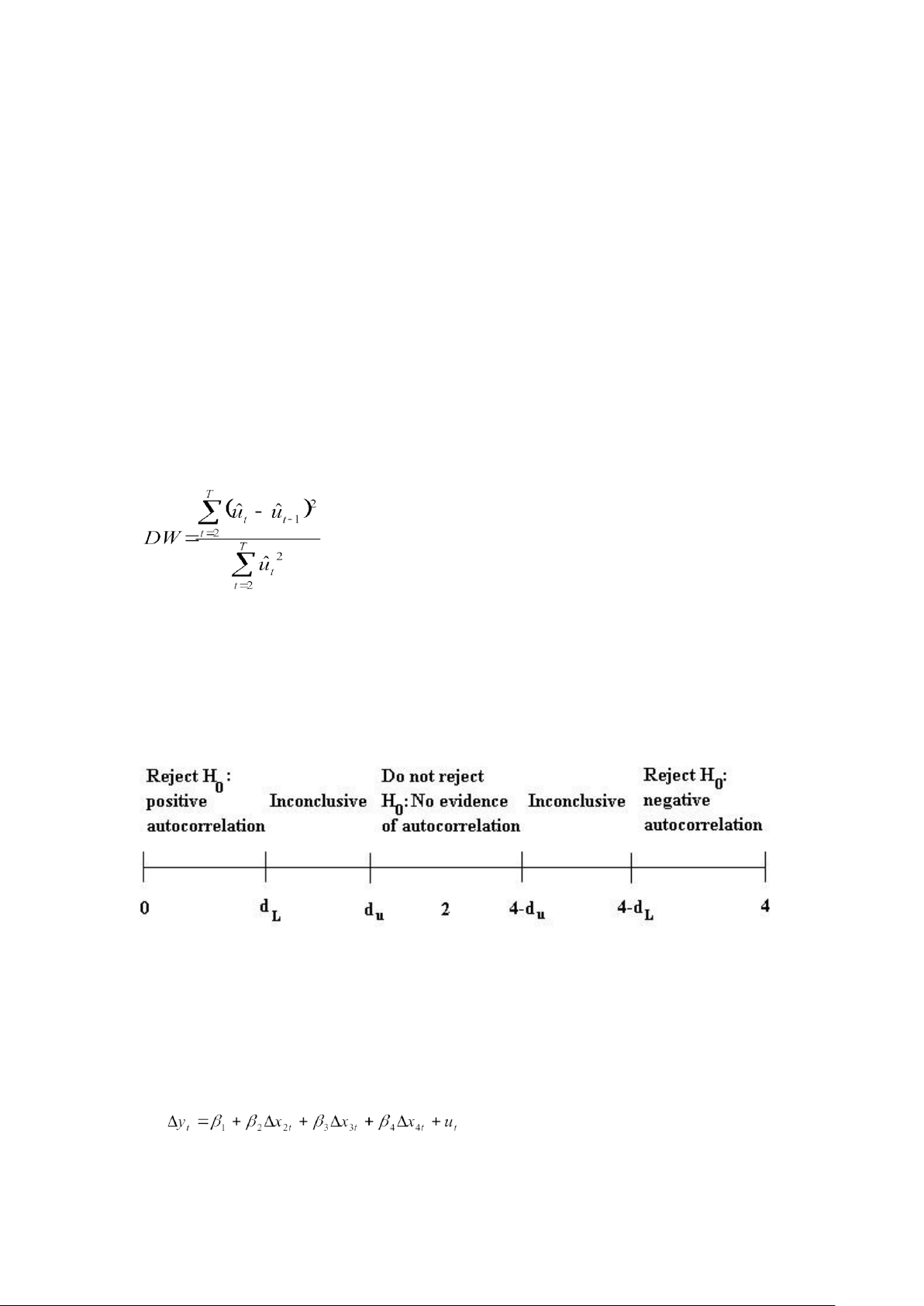
The Durbin Watson test is a test for first order autocorrelation. The test
iscalculated as follows. You would run whatever regression you were interested in, and
obtain the residuals. Then calculate the statistic
You would then need to look up the two critical values from the Durbin Watson tables,
and these would depend on how many variables and how many observations and how
many regressors (excluding the constant this time) you had in the model.
The rejection / non-rejection rule would be given by selecting the appropriate region from the following diagram: (c)
We have 60 observations, and the number of regressors excluding the
constantterm is 3. The appropriate lower and upper limits are 1.48 and 1.69
respectively, so the Durbin Watson is lower than the lower limit. It is thus clear that we
reject the null hypothesis of no autocorrelation. So it looks like the residuals are positively autocorrelated. (d) lOMoAR cPSD| 58583460
The problem with a model entirely in first differences, is that once we calculate the long
run solution, all the first difference terms drop out (as in the long run we assume that
the values of all variables have converged on their own long run values so that yt = yt-1
etc.) Thus when we try to calculate the long run solution to this model, we cannot do it because there isn’t a long run solution to this model! (e)
The answer is yes, there is no reason why we cannot use Durbin Watson in this case.
You may have said no here because there are lagged values of the regressors (the x
variables) variables in the regression. In fact this would be wrong since there are no
lags of the DEPENDENT (y) variable and hence DW can still be used. 6.
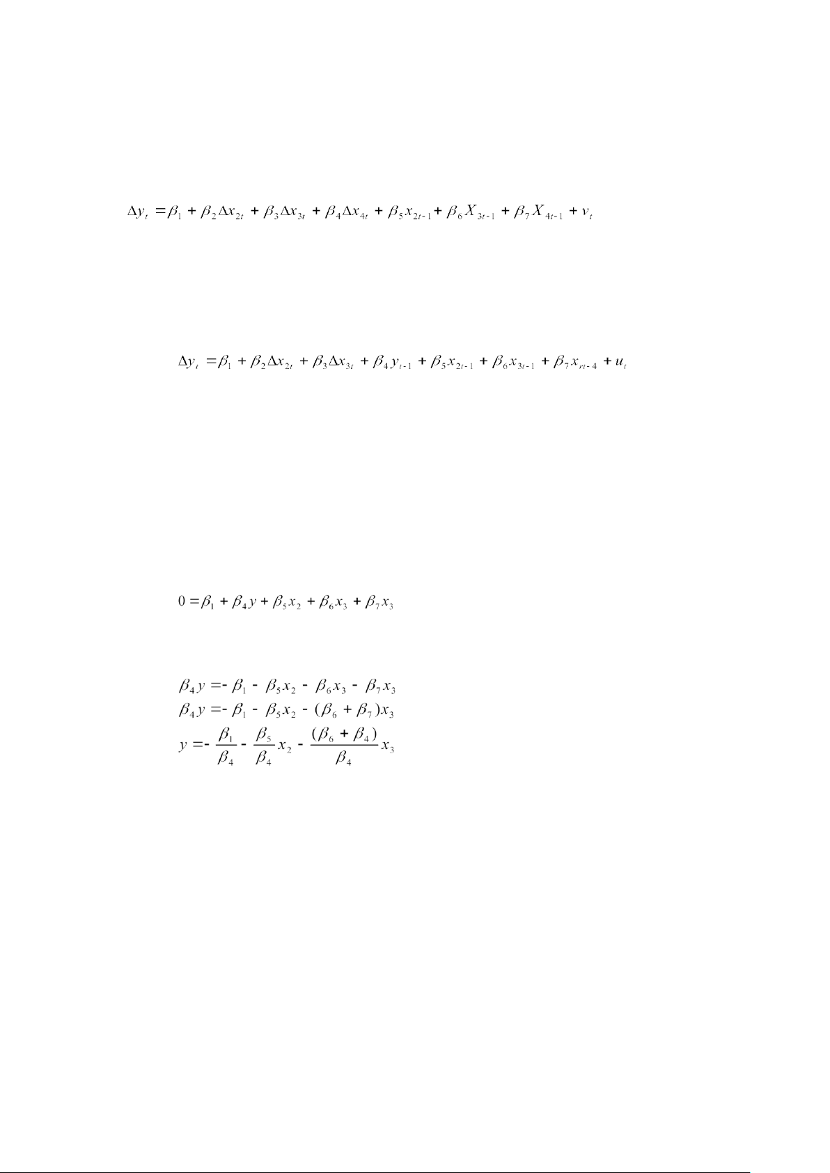
The major steps involved in calculating the long run solution are to
- set the disturbance term equal to its expected value of zero - drop the time subscripts
- remove all difference terms altogether since these will all be zero by the definitionof the long run in this context.
Following these steps, we obtain
We now want to rearrange this to have all the terms in x2 together and so that y is the subject of the formula:
The last equation above is the long run solution. 7.
Ramsey’s RESET test is a test of whether the functional form of the regression
isappropriate. In other words, we test whether the relationship between the dependent
variable and the independent variables really should be linear or whether a non-linear
form would be more appropriate. The test works by adding powers of the fitted values
from the regression into a second regression. If the appropriate model was a linear one,
then the powers of the fitted values would not be significant in this second regression.
If we fail Ramsey’s RESET test, then the easiest “solution” is probably to transform all
of the variables into logarithms. This has the effect of turning a multiplicative model into an additive one. lOMoAR cPSD| 58583460
If this still fails, then we really have to admit that the relationship between the dependent
variable and the independent variables was probably not linear after all so that we have
to either estimate a non-linear model for the data (which is beyond the scope of this
course) or we have to go back to the drawing board and run a different regression
containing different variables. 8.
(a) It is important to note that we did not need to assume normality in order
toderive the sample estimates of and or in calculating their standard errors. We
needed the normality assumption at the later stage when we come to test hypotheses
about the regression coefficients, either singly or jointly, so that the test statistics we
calculate would indeed have the distribution (t or F) that we said they would.
(b) One solution would be to use a technique for estimation and inference which did not
require normality. But these techniques are often highly complex and also their
properties are not so well understood, so we do not know with such certainty how well
the methods will perform in different circumstances.
One pragmatic approach to failing the normality test is to plot the estimated residuals
of the model, and look for one or more very extreme outliers. These would be residuals
that are much “bigger” (either very big and positive, or very big and negative) than the
rest. It is, fortunately for us, often the case that one or two very extreme outliers will
cause a violation of the normality assumption. The reason that one or two extreme
outliers can cause a violation of the normality assumption is that they would lead the
(absolute value of the) skewness and / or kurtosis estimates to be very large.
Once we spot a few extreme residuals, we should look at the dates when these outliers
occurred. If we have a good theoretical reason for doing so, we can add in separate
dummy variables for big outliers caused by, for example, wars, changes of government,
stock market crashes, changes in market microstructure (e.g. the “big bang” of 1986).
The effect of the dummy variable is exactly the same as if we had removed the
observation from the sample altogether and estimated the regression on the remainder.
If we only remove observations in this way, then we make sure that we do not lose any
useful pieces of information represented by sample points.
9. (a) Parameter structural stability refers to whether the coefficient estimates for a
regression equation are stable over time. If the regression is not structurally stable, it
implies that the coefficient estimates would be different for some sub-samples of the
data compared to others. This is clearly not what we want to find since when we
estimate a regression, we are implicitly assuming that the regression parameters are
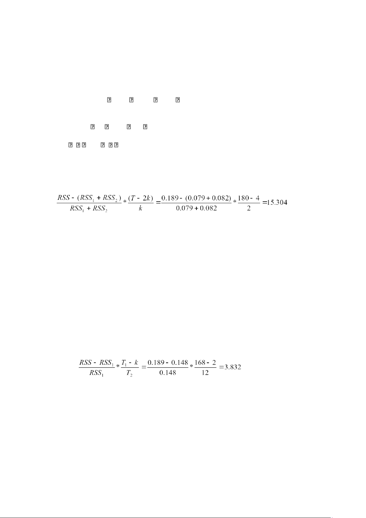
constant over the entire sample period under consideration. (b) 1981M1-1995M12
rt = 0.0215 + 1.491 rmt RSS=0.189 T=180 lOMoAR cPSD| 58583460 1981M1-1987M10
rt = 0.0163 + 1.308 rmt 1987M11- RSS=0.079 T=82 1995M12
rt = 0.0360 + 1.613 rmt RSS=0.082 T=98 (c)
If we define the coefficient estimates for the first and second halves of the
sampleas 1 and 1, and 2 and 2 respectively, then the null and alternative hypotheses are H0 : 1 = 2 and 1 = 2 and H1 : 1 2 or 1 2 (d)
The test statistic is calculated as Test stat. =
This follows an F distribution with (k,T-2k) degrees of freedom. F(2,176) = 3.05 at the
5% level. Clearly we reject the null hypothesis that the coefficients are equal in the two sub-periods.
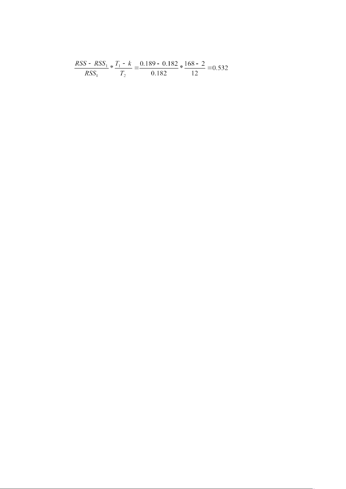
10. The data we have are 1981M1- 1995M12
rt = 0.0215 + 1.491 Rmt RSS=0.189 T=180 1981M1-1994M12
rt = 0.0212 + 1.478 Rmt RSS=0.148 T=168 1982M1-1995M12
rt = 0.0217 + 1.523 Rmt RSS=0.182 T=168
First, the forward predictive failure test - i.e. we are trying to see if the model for
1981M1-1994M12 can predict 1995M1-1995M12.
The test statistic is given by
Where T1 is the number of observations in the first period (i.e. the period that we
actually estimate the model over), and T2 is the number of observations we are trying
to “predict”. The test statistic follows an F-distribution with (T2, T1-k) degrees of
freedom. F(12, 166) = 1.81 at the 5% level. So we reject the null hypothesis that the
model can predict the observations for 1995. We would conclude that our model is no
use for predicting this period, and from a practical point of view, we would have to
consider whether this failure is a result of a-typical behaviour of the series out-ofsample
(i.e. during 1995), or whether it results from a genuine deficiency in the model. lOMoAR cPSD| 58583460
The backward predictive failure test is a little more difficult to understand, although no
more difficult to implement. The test statistic is given by
Now we need to be a little careful in our interpretation of what exactly are the “first”
and “second” sample periods. It would be possible to define T1 as always being the first
sample period. But I think it easier to say that T1 is always the sample over which we
estimate the model (even though it now comes after the hold-out-sample). Thus T2 is
still the sample that we are trying to predict, even though it comes first. You can use
either notation, but you need to be clear and consistent. If you wanted to choose the
other way to the one I suggest, then you would need to change the subscript 1
everywhere in the formula above so that it was 2, and change every 2 so that it was a 1.
Either way, we conclude that there is little evidence against the null hypothesis. Thus
our model is able to adequately back-cast the first 12 observations of the sample. 11.
By definition, variables having associated parameters that are not
significantlydifferent from zero are not, from a statistical perspective, helping to
explain variations in the dependent variable about its mean value. One could therefore
argue that empirically, they serve no purpose in the fitted regression model. But leaving
such variables in the model will use up valuable degrees of freedom, implying that the
standard errors on all of the other parameters in the regression model, will be
unnecessarily higher as a result. If the number of degrees of freedom is relatively small,
then saving a couple by deleting two variables with insignificant parameters could be
useful. On the other hand, if the number of degrees of freedom is already very large,
the impact of these additional irrelevant variables on the others is likely to be inconsequential. 12.
An outlier dummy variable will take the value one for one observation in
thesample and zero for all others. The Chow test involves splitting the sample into two
parts. If we then try to run the regression on both the sub-parts but the model contains
such an outlier dummy, then the observations on that dummy will be zero everywhere
for one of the regressions. For that sub-sample, the outlier dummy would show perfect
multicollinearity with the intercept and therefore the model could not be estimated.