Economics Chapters 1-9: Key Principles and Concepts Explained | Microeconomics | Trường Đại học Quốc tế, Đại học Quốc gia Thành phố Hồ Chí Minh

Chapter 1 Ten Principles of Economics Scarcity Economics 1. How people make decisions
1.1.1. Principle 1: People face Trade-offs Efficiency Equality
1.1.2. Principle 2: The Cost of something is what you Give up to Get it Opportunity cost
1.1.3. Principle 3: Rational People think at the Margin Rational people Marginal change o Marginal Cost (MC) o Marginal Benefit (MB)
People only make decisions if MB>MC Willingness to Pay
1.1.4. Principle 4: People Respond to Incentives Incentive 2. How people interact
1. Principle 5: Trade can make Everyone Better Off Comparative Advantage Absolute Advantage
2. Principle 6: Markets are Usually a Good Way to Organize Economic Activity Market Market Economy Invisible Hand by Adam Smith
3. Principle 7: Governments can Sometimes Improve Market Outcomes Property Rights Market failure o Externality o Market power
3. How the Economy as a Whole Works
1. Principle 8: A country’s Standard of Living Depends on its Ability to Produce Goods and Services Productivity
2. Principle 9: Prices Rise when the Government Prints Too Much Money Inflation
3. Principle 10: Society Faces a Short-run Trade-off between Inflation and Unemployment
Chapter 2 Thinking Like an Economist
1. The Economist as a Scientist The Scientific Method Assumptions Models o
First Model: Circular-Flow Diagram o
Second Model: The PPF (Production Possibilities Frontier)
Economic growth shifts PPF outward Shape of PPF
Straight: constant opportunity cost
Bowed outward: increasing opportunity cost Why bowed outward Workers have different skills Different opportunity costs
Microeconomics and Macroeconomics
2. The Economist as Policy Adviser Positive vs Normative 3. Why Economists Disagree
Chapter 3 Interdependence and the Gains from Trade
1. A Parable for the Modern Economy
3.1.1. Production Possibilities
3.1.2. Specialization and Trade 2. Comparative Advantage 3.2.1. Absolute Advantage Using fewer inputs
3.2.2. Opportunity Cost and Comparative Advantage Lower Opportunity cost
3.2.3. Comparative Advantage and Trade
Chapter 4 The Market Forces of Supply and Demand 1. Markets and Competition 1. What is a Market? 2. What is Competition?
Competitive Market: everyone has small impact on market price
Perfectly competitive market: no impact on market price 2. Demand
1. The Demand Curve: The relationship between Price and Quantity Demanded Quantity demanded Law of demand o
Price rises, quantity demanded falls o
Price falls, quantity demanded rises
2. Market Demand vs Individual Demand Market Demand 3. Shifts in the Demand Curve Demand Curve
o Shows how price affects Qd (quantity demanded), other things being equal Number of buyers
o Increase in number of buyers -> increase Qd -> shift D curve to right
o Decrease in number of buyers -> decrease Qd -> shift D curve to left Income
o Normal good: increase in income -> increase in demand
o Inferior good: increase in income -> decrease in demand Substitutes
o Two goods are substitutes if: increase in price of one -> increase in demand for other
o Ex: pizza and hamburger: increase in pizza price -> increase in demand for hamburger Complements
o Two goods are complements if: increase in price of one -> decrease in demand for other
o Ex: computer and software: price of comp rises -> people buy less comps -> less software
o Other exes: egg and bacon, college tuition and textbook, bagel and cream cheese, peanut butter and jelly Tastes
o A shift in tastes -> increase demand
o Ex: Atkin diet popular -> increase in demand for eggs Expectations about future
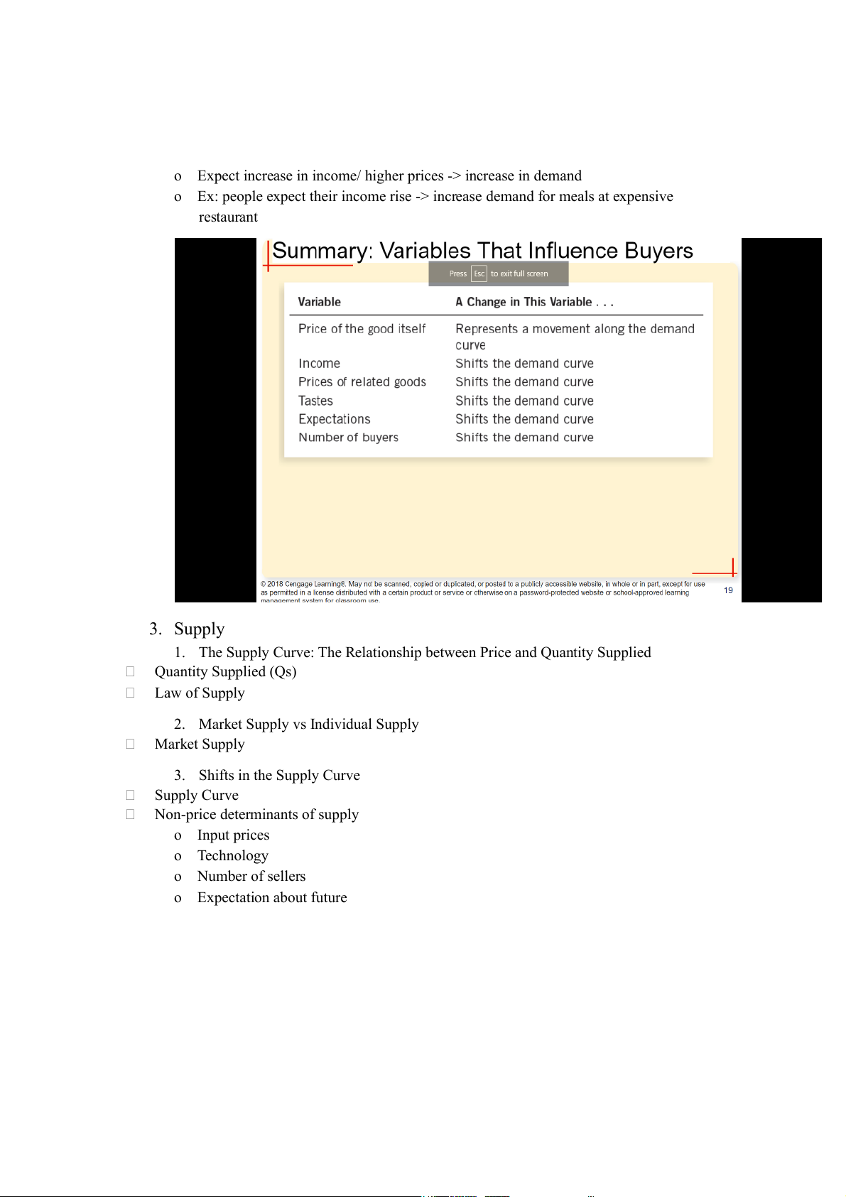
o Expect increase in income/ higher prices -> increase in demand
o Ex: people expect their income rise -> increase demand for meals at expensive restaurant 3. Supply
1. The Supply Curve: The Relationship between Price and Quantity Supplied Quantity Supplied (Qs) Law of Supply
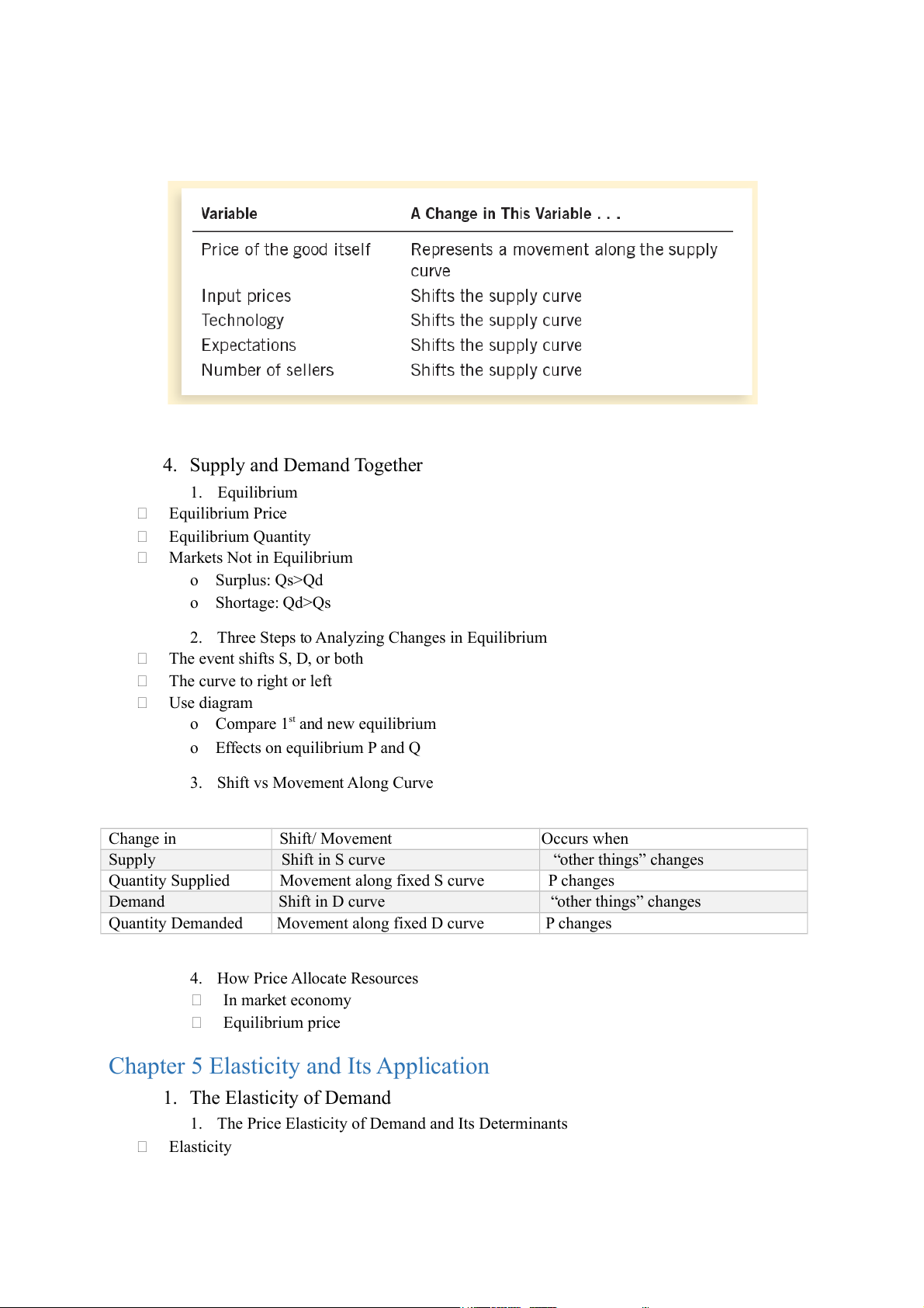
2. Market Supply vs Individual Supply Market Supply 3. Shifts in the Supply Curve Supply Curve
Non-price determinants of supply o Input prices o Technology o Number of sellers o Expectation about future 4. Supply and Demand Together 1. Equilibrium Equilibrium Price Equilibrium Quantity Markets Not in Equilibrium o Surplus: Qs>Qd o Shortage: Qd>Qs
2. Three Steps to Analyzing Changes in Equilibrium The event shifts S, D, or both The curve to right or left Use diagram
o Compare 1st and new equilibrium
o Effects on equilibrium P and Q
3. Shift vs Movement Along Curve Change in Shift/ Movement Occurs when Supply Shift in S curve “other things” changes Quantity Supplied Movement along fixed S curve P changes Demand Shift in D curve “other things” changes Quantity Demanded Movement along fixed D curve P changes
4. How Price Allocate Resources In market economy Equilibrium price
Chapter 5 Elasticity and Its Application 1. The Elasticity of Demand
1. The Price Elasticity of Demand and Its Determinants Elasticity Price Elasticity of Demand Determinants o Close substitutes o Narrowly defined o Luxury o Long Run
2. Computing the Price Elasticity of Demand Price Elasticity of Demand =
Calculating Percentage Change = x 100% 3. The Midpoint Method
Midpoint: number halfway between start and end value
4. The Variety of Demand Curves Elastic: Edp > 1 Inelastic: Edp < 1 Unit elastic: Edp = 1 Perfect inelastic: Edp = 0 Perfect elastic: Edp = ∞
Flatter D curve -> greater Edp
5. Total Revenue and the Price Elasticity of Demand Total Revenue = P x Q o Higher TR: Higher P o Lower TR: Lower Q
o Increase: if P increase, demand inelastic
o Decrease: if P increase, demand elastic
6. Elasticity and Total Revenue along a Linear Demand Curve
The slope of linear D curve is constant, but not its elasticity 7. Other Demand Elasticities Income elasticity of Demand
o Normal good: income elasticity > 0
o Inferior good: income elasticity < 0
Cross-price elasticity of Demand
o Substitutes: cross-price elasticity > 0
o Complements: cross-price elasticity < 0 2. The Elasticity of Supply
1. The Price Elasticity of Supply and Its Determinants Price Elasticity of Supply Determinants
o More easily sellers change quantity o Long run
2. Computing the Price Elasticity of Supply Price elasticity of Supply =
3. The Variety of Supply Curves Unit elastic: Esp = 1 Elastic: Esp > 1 Inelastic: Esp < 1 Perfectly inelastic: Esp = 0 Perfectly elastic: Esp = ∞
Flatter S curve -> greater Esp 3. Applications
Chapter 6 Supply, Demand and Government Policies 1. Control on Prices
1. How Price Ceilings Affect Market Outcomes
Price Ceiling (rent-control laws) Must be below equilibrium Create shortage
2. How Price Floors Affect Market Outcomes Price floor (minimum wage) Must be above equilibrium Create surplus 3. Evaluating Price Controls
Markets are usually a good way to organize economic activity
o Economists usually oppose price controls
Governments can sometimes improve market outcomes 2. Taxes
The Outcome is the Same in Both Cases: equilibrium quantity falls
1. How Taxes on Sellers Affect Market Outcomes Shift S curve up
2. How Taxes on Buyers Affect Market Outcomes Shift D curve down
3. Elasticity and Tax Incidence Tax incidence
Supply more elastic than demand: Buyers bear most of tax burden
Demand more elastic than supply: Sellers bear most of tax burden
Chapter 7 Consumers, Producers, and the Efficiency of Markets Welfare economics 1. Consumer Surplus Willingness to Pay Marginal buyer
Consumer surplus = Willingness to Pay – Price Consumer surplus o Under the D curve o Above P Higher price Reduces CS 2. Producer Surplus Cost Marginal seller
Producer Surplus = Price – Cost Producer Surplus o Above the S curve o Under P Lower Price reduces PS 3. Market Efficiency Total surplus = CS + PS
Total surplus = Value to buyers – Cost to sellers
o Consumer surplus = Value to buyers – Amount paid by buyers
o Produces Surplus = Amount received by sellers – Cost to sellers
Market’s Allocation of Resources o Decentralized
o Total surplus -> whether market’s allocation is efficient
o Efficient allocation of resources maximizes total surplus Invisible hand Free markets Market Failures o Market Power o Externality
Chapter 8 Application: The Costs of Taxation
1. The Deadweight Loss of Taxation
Tax reduces welfare of buyers and sellers
Welfare loss > the Tax Revenue (usually)
2. The Determinants of the Deadweight Loss
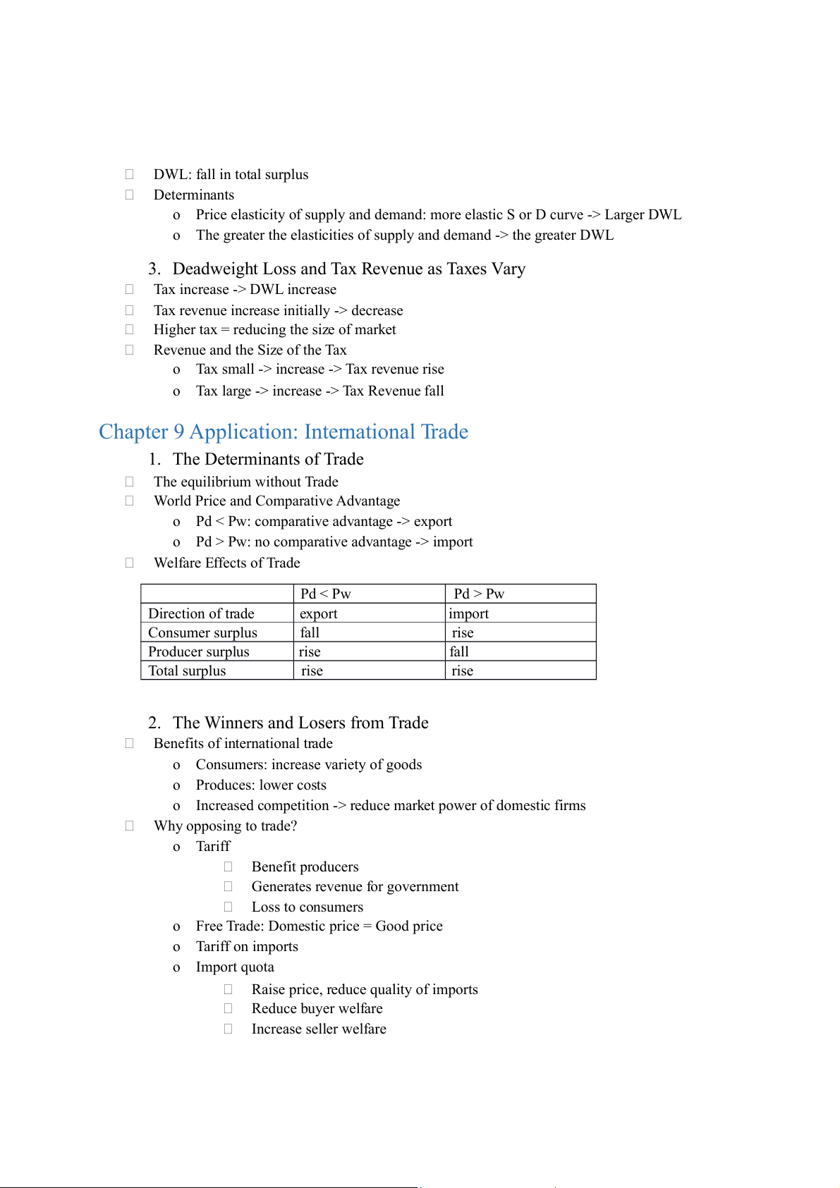
Revenue from Tax = Size of Tax x Quantity sold DWL: fall in total surplus Determinants
o Price elasticity of supply and demand: more elastic S or D curve -> Larger DWL
o The greater the elasticities of supply and demand -> the greater DWL
3. Deadweight Loss and Tax Revenue as Taxes Vary
Tax increase -> DWL increase
Tax revenue increase initially -> decrease
Higher tax = reducing the size of market
Revenue and the Size of the Tax
o Tax small -> increase -> Tax revenue rise
o Tax large -> increase -> Tax Revenue fall
Chapter 9 Application: International Trade 1. The Determinants of Trade The equilibrium without Trade
World Price and Comparative Advantage
o Pd < Pw: comparative advantage -> export
o Pd > Pw: no comparative advantage -> import Welfare Effects of Trade Pd < Pw Pd > Pw Direction of trade export import Consumer surplus fall rise Producer surplus rise fall Total surplus rise rise
2. The Winners and Losers from Trade
Benefits of international trade
o Consumers: increase variety of goods o Produces: lower costs
o Increased competition -> reduce market power of domestic firms Why opposing to trade? o Tariff Benefit producers
Generates revenue for government Loss to consumers
o Free Trade: Domestic price = Good price o Tariff on imports o Import quota
Raise price, reduce quality of imports Reduce buyer welfare Increase seller welfare
3. The Arguments for Restricting Trade Jobs argument National-security argument Infant-industry argument Unfair-competition argument
Protection-as-a-bargaining-chip argument