Elasticity Concepts and Examples | Microeconomics | Trường Đại học Quốc tế, Đại học Quốc gia Thành phố Hồ Chí Minh

E= ∆ X % ∆ Y %
+ E = 5: Y increases by 1% => X increases by 5%: X is very sensitive to changes in Y
+ E = -0.5: Y increases by 1% => X decreases by 0.5%: X is very insensitive to changes in Y
Price elasticity of demand (EDP) ∆ Q % E = D DP ∆ P %
Law of demand: P increases/decreases => QD decreases/increases => EDP < 0
+ EDP = - 5: P increases by 1% => QD decreases by 5%: Buyers are very sensitive to changes in price
+ EDP = -0.1: P increases by 1% => QD decreases by 0.1%: Buyers are
very insensitive to changes in price
Mid point method: A and B
(Q −Q ) (P +P )/2 E = 2 1 2 1 . DP
(P −P ) (Q +Q )/2 2 1 2 1 (8400 10600 − ) (600 4000 2 + )/ E = . =−0.58 DP (600−400) (8400+10600)/2 Point elasticity:
Points A and B approach each other -> AB can be considered as a point P E = dQ . DP dP Q P E =Q ' . DP P Q 1 P E = . DP P ' Q Q Demand function: D: QD = a – bP P E =−b . DP Q D: P = c – dQD 1 P E = . DP −d Q Ex1: D: QD = 100 – 10P
At point A (P = 5$, Q = 50 units) 5 E =−10. =−1 DP 50 Ex2:
At point A (P = 40$, Q = 10 units) EDP at point A = -0.5 What is demand function? D: P = a – bQD 1 P E = . DP −b Q 1 40 −0.5= . =¿ b=8 −b 10 D : P = a – 8QD 40 = a – 8.10 => a = 120 D: P = 120 – 8QD D: QD = 15 – 0.125P ∆ Q % E = D DP ∆ P %
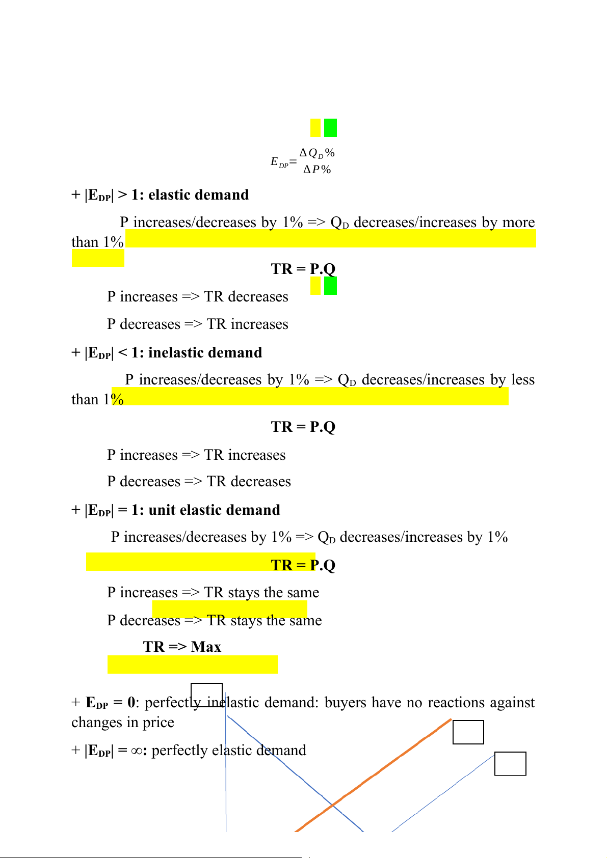
+ |EDP| > 1: elastic demand
P increases/decreases by 1% => QD decreases/increases by more than 1% TR = P.Q P increases => TR decreases P decreases => TR increases
+ |EDP| < 1: inelastic demand
P increases/decreases by 1% => QD decreases/increases by less than 1% TR = P.Q P increases => TR increases P decreases => TR decreases
+ |EDP| = 1: unit elastic demand
P increases/decreases by 1% => QD decreases/increases by 1% TR = P.Q
P increases => TR stays the same
P decreases => TR stays the same TR => Max
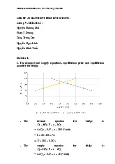
+ EDP = 0: perfectly inelastic demand: buyers have no reactions against changes in price + |EDP perfectly elast | = ∞: ic demand Agricultural production
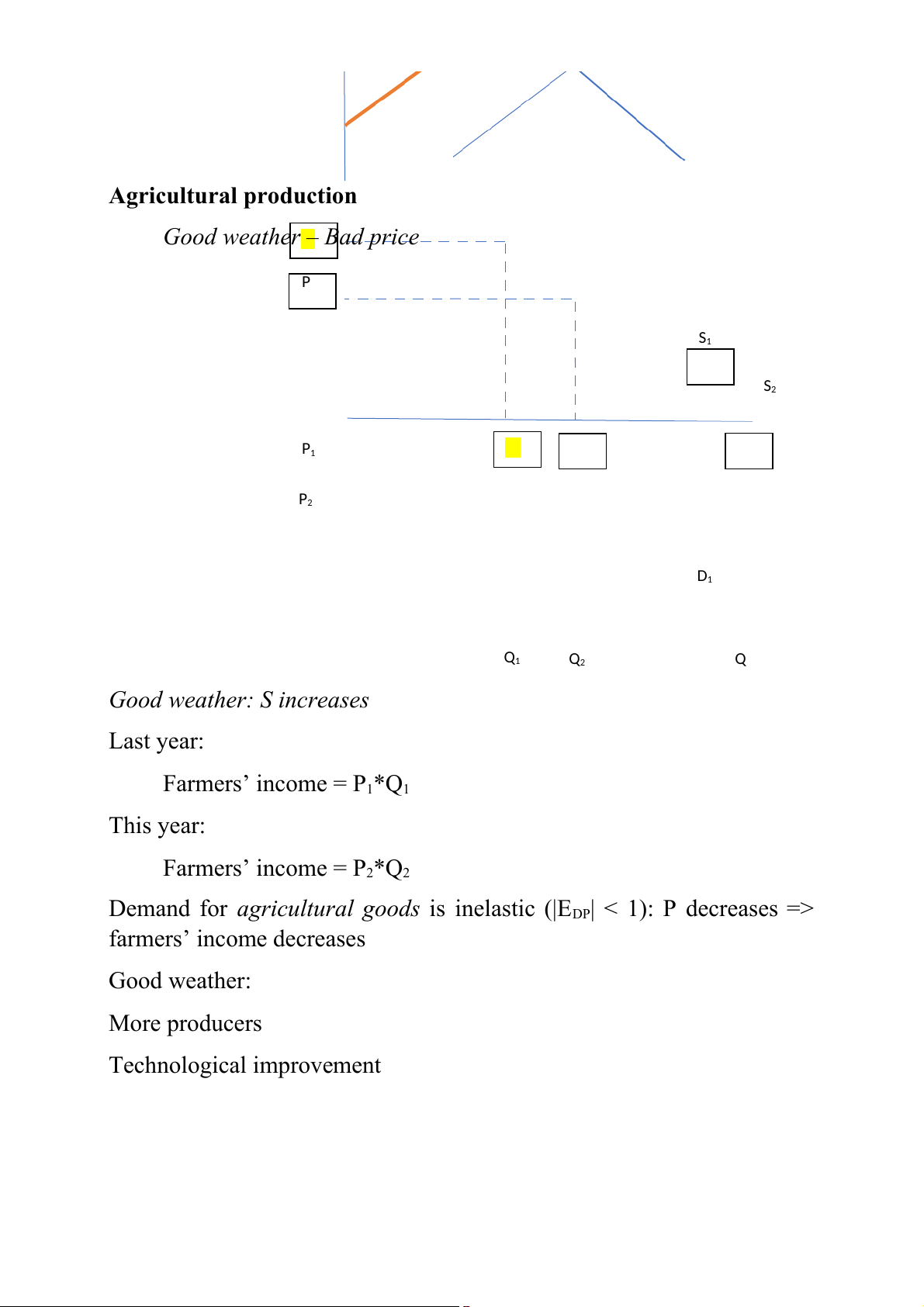
Good weather – Bad price P S1 S2 P1 P2 D1 Q1 Q2 Q
Good weather: S increases Last year: Farmers’ income = P1*Q1 This year: Farmers’ income = P2*Q2
Demand for agricultural
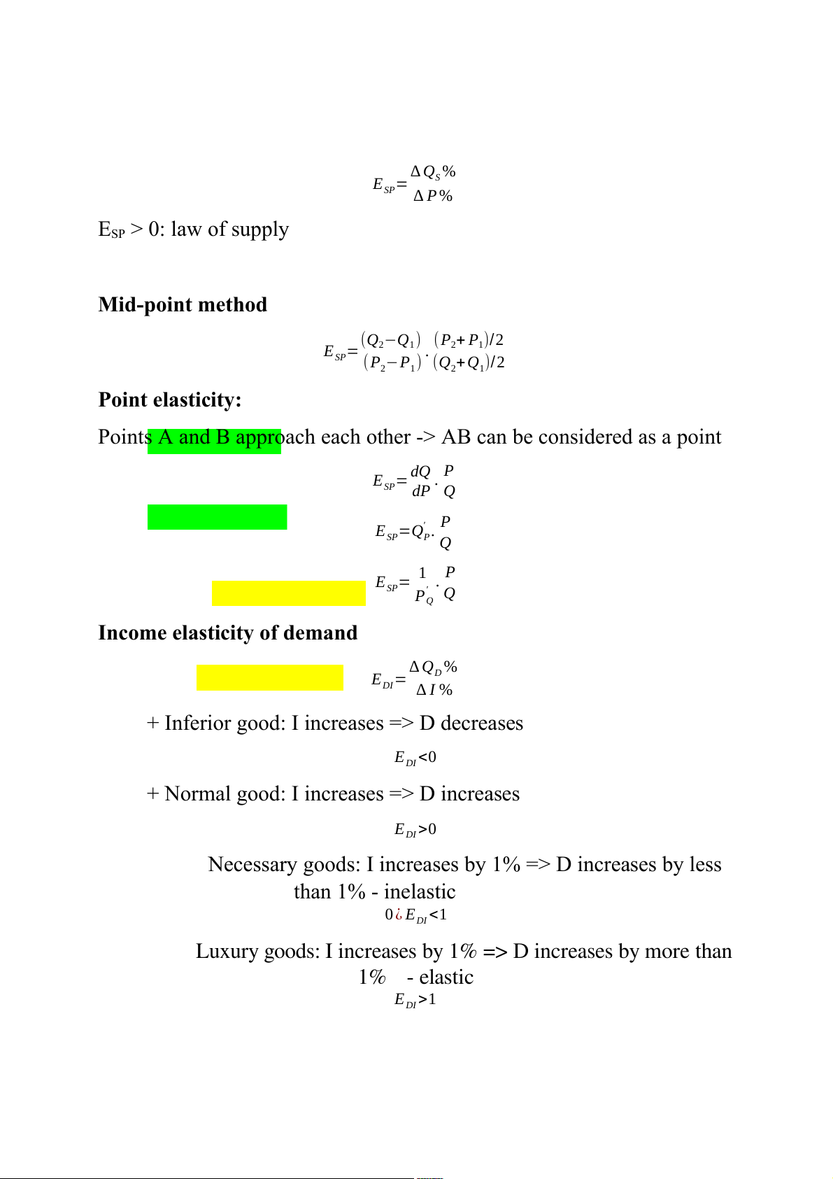
goods is inelastic (|EDP| < 1): P decreases => farmers’ income decreases Good weather: More producers Technological improvement ∆ Q % E = S SP ∆ P % ESP > 0: law of supply Mid-point method
(Q −Q ) (P + P )/2 2 1 E = 2 1 . SP
(P −P ) (Q + Q )/2 2 1 2 1 Point elasticity:
Points A and B approach each other -> AB can be considered as a point P E = dQ . SP dP Q P E =Q' . SP P Q 1 P E = . SP P' Q Q
Income elasticity of demand ∆ Q % E = D DI ∆ I %
+ Inferior good: I increases => D decreases E <0 DI
+ Normal good: I increases => D increases E >0 DI
Necessary goods: I increases by 1% => D increases by less than 1% - inelastic 0 ¿ E <1 DI
Luxury goods: I increases by 1% => D increases by more than 1% - elastic E >1 DI
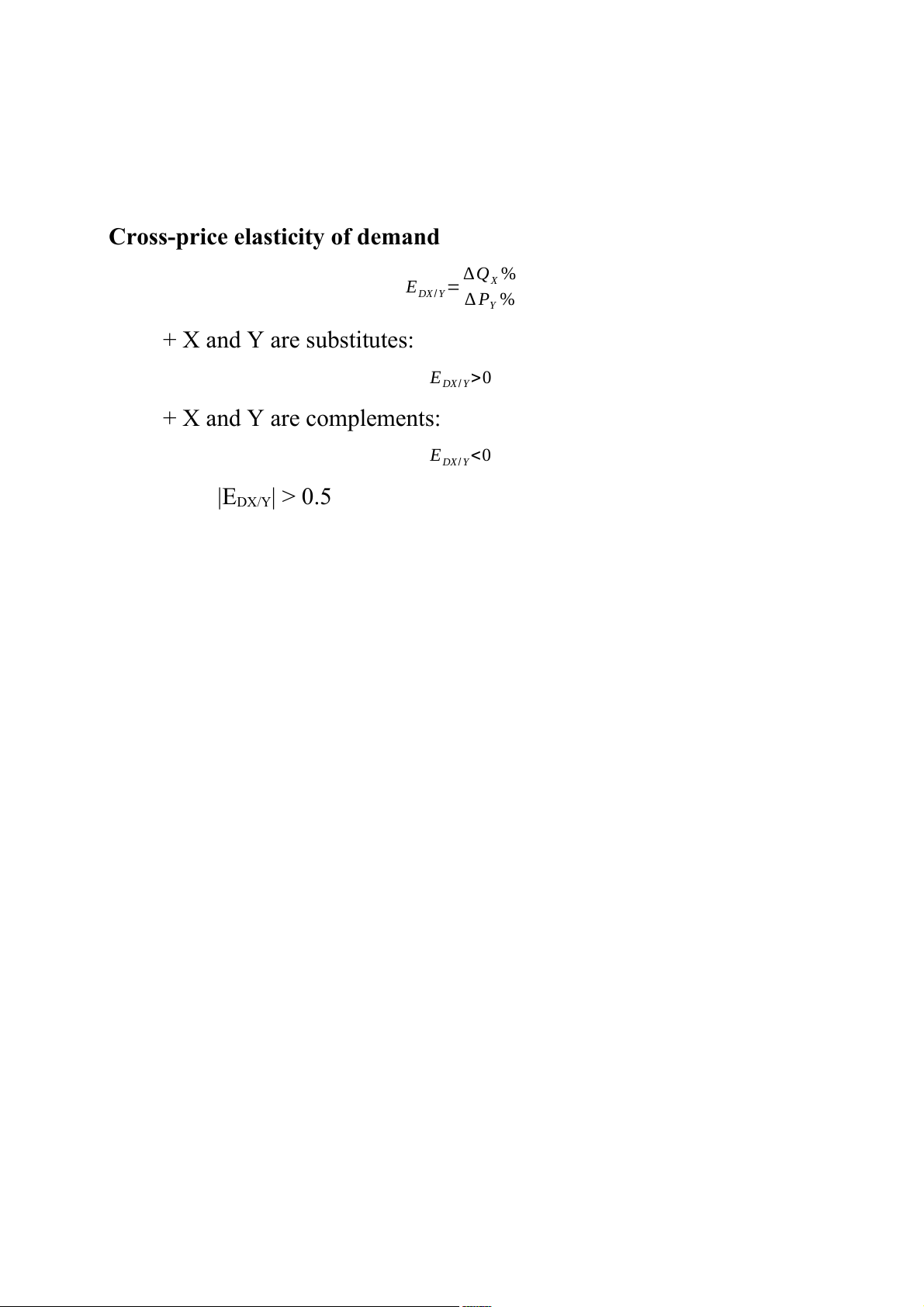
Cross-price elasticity of demand ∆ Q % E = X DX / Y ∆ P % Y + X and Y are substitutes: E >0 DX / Y + X and Y are complements: E <0 DX / Y |EDX/Y| > 0.5