Kinh tế vi mô Assignment 2: Demand and Supply Analysis | Microeconomics | Trường Đại học Quốc tế, Đại học Quốc gia Thành phố Hồ Chí Minh

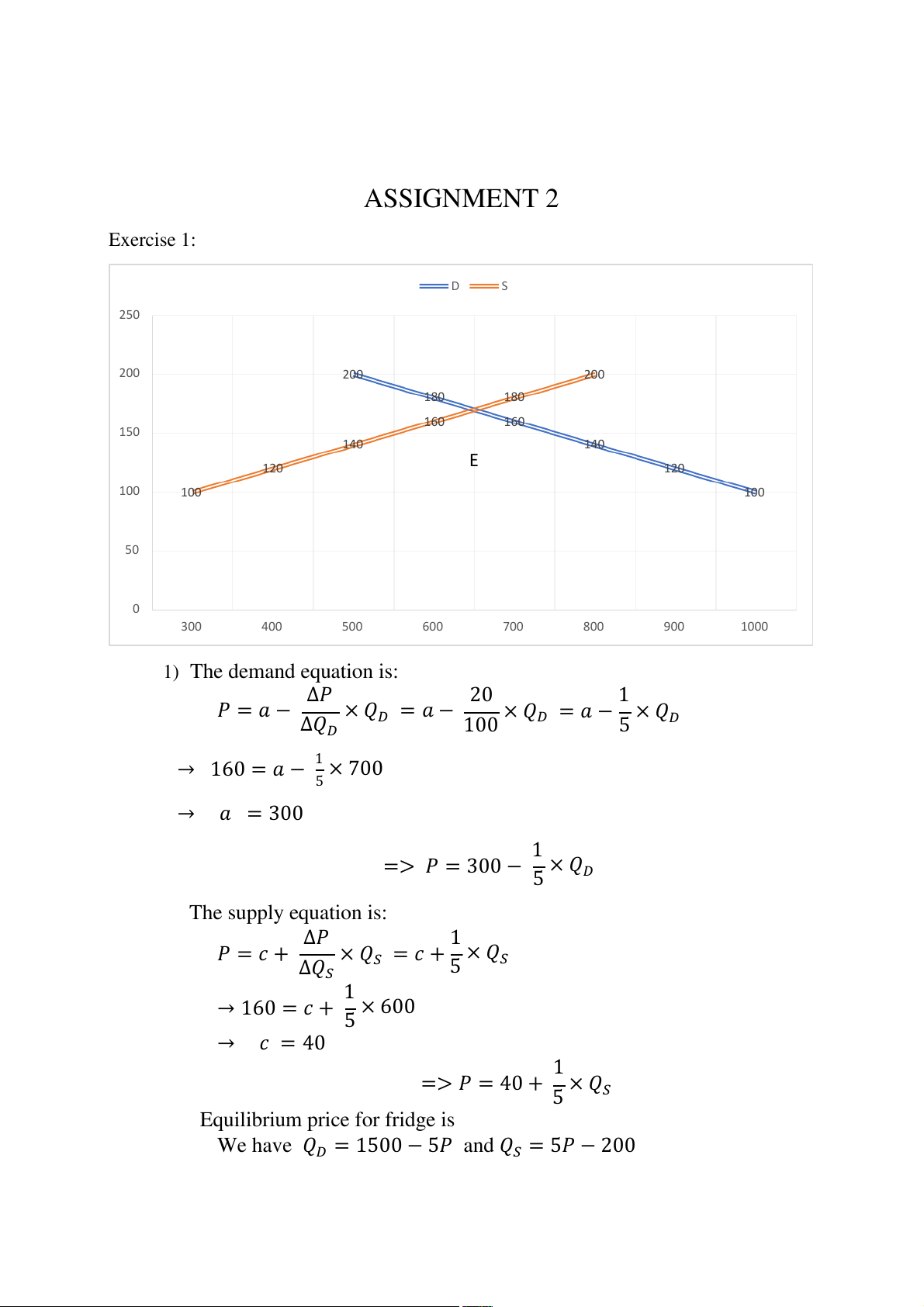
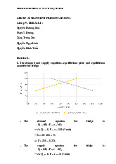
ASSIGNMENT 2 Exercise 1: D S 250 200 200 200 180 180 160 160 150 140 140 E 120 120 100 100 100 50 0 300 400 500 600 700 800 900 1000 1) The demand equation is: Δ𝑃 20 1 𝑃 = 𝑎 − × 𝑄 × 𝑄 × 𝑄 Δ𝑄 𝐷 = 𝑎 − 𝐷 = 𝑎 − 𝐷 𝐷 100 5 1 → 160 = 𝑎 − × 700 5 → 𝑎 = 300 1 => 𝑃 = 300 − × 𝑄 5 𝐷 The supply equation is: Δ𝑃 1 𝑃 = 𝑐 + × 𝑄 × 𝑄 Δ𝑄 𝑆 = 𝑐 + 5 𝑆 𝑆 1 → 160 = 𝑐 + × 600 5 → 𝑐 = 40 1 => 𝑃 = 40 + × 𝑄 5 𝑆
Equilibrium price for fridge is
We have 𝑄𝐷 = 1500 − 5𝑃 and 𝑄𝑆 = 5𝑃 − 200
And 𝑄𝐸 = 𝑄𝐷 = 𝑄𝑆 → 𝑄𝐷 − 𝑄𝑆 = 0
→ 1500 − 5𝑃 − 5𝑃 + 200 = 0 → 𝑃𝐸 = $170
Equilibrium quantity for fridge is
𝑄𝐸 = 𝑄𝐷 → 𝑄𝐸 = 1500 − 5 × 170 = 650 → 𝑄𝐸 = 650 (units)
2) At the price of $200, we have
𝑄𝑆 = 5 × 200 − 200 = 800 (units)
𝑄𝐷 = 1500 − 5 × 200 = 500 (units) → 𝑄 → Surplus 𝑆 > 𝑄𝐷
→ The surplus at the price of $200 is
𝑄𝑆 − 𝑄𝐷 = 800 − 500 = 300 (units)
At the price of $110, we have
𝑄𝑆 = 5 × 110 − 200 = 350 (units)
𝑄𝐷 = 1500 − 5 × 110 = 950 (units) → 𝑄 → Shortage 𝐷 > 𝑄𝑆
→ The shortage at the price of $110 is
𝑄𝐷 − 𝑄𝑆 = 950 − 350 = 600 (units)
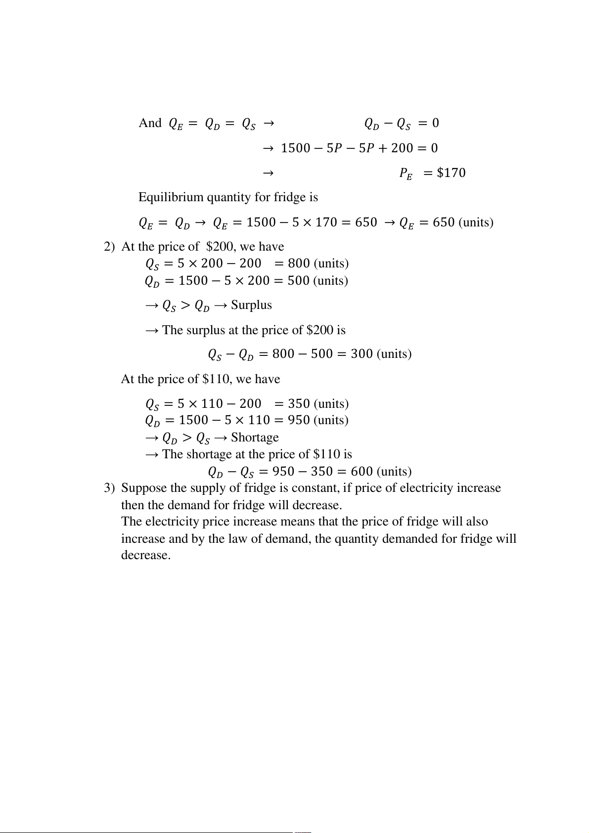
3) Suppose the supply of fridge is constant, if price of electricity increase
then the demand for fridge wil decrease.
The electricity price increase means that the price of fridge will also
increase and by the law of demand, the quantity demanded for fridge will decrease. D S D' 250 200 200 200 180 180 160 160 150 140 140 120 120 PRICE ($) 100 100 100 50 0 300 400 500 600 700 800 900 1000 QUANTITY (UNITS)
If quantity demanded for fridge decrease 300 units at each price level,
then the new demand line will move to the left, paralled with the initial demand line. → 𝑄′ = 𝑄 𝐷
𝐷 − 300 = 1500 − 5𝑃 − 300 = 1200 − 5𝑃
→ 𝑄′𝐷 = 1200 − 5𝑃
The new equilibrium price for fridge is 𝑄′ 𝐷 = 𝑄𝑆 ′
→ 1200 − 5𝑃 = 5𝑃 − 200 → 𝑃𝐸 = $140
→ The new equilibrium quantity is 𝑄′𝐷 = 1200 − 5 × 140 = 500 (units)
4) If the government imposes a tax of $ 10 per one units of fridge sold then
the price of demand will increase 1
→ 𝑃 = 40 + × 𝑄 5 𝑆 + 10
→ 𝑄′′𝑆 = 5𝑃 − 250
The new equilibrium price for this scenerio is 𝑄′′
→ −1500 + 5𝑃 + 5P − 250 = 0 𝑆 = 𝑄𝐷 → −1750 + 10𝑃 = 0 → 𝑃′′𝐸 = $175
The new equilibrium quatity is 𝑄′′ ′′ ′′ = 5 × 175 − 250 𝐸 = 𝑄𝑆 → 𝑄𝐸
→ 𝑄′′𝐸 = 625 (units)
5) Suppose government supports for the sellers the amount of $ 10 per one units of fridge sold 1 → 𝑃 = 40 + × 𝑄 5 𝑆 − 10 → 𝑄′′′ 𝑆 = 5𝑃 − 150
The new equilibrium price for this sistuation is 𝑄′′′
→ −1500 + 5𝑃 − 150 + 5P = 0 𝑆 = 𝑄𝐷 → 10𝑃 = 165 0 → 𝑃′′′ 𝐸 = $165
The new equilibrium quatity is 𝑄′′′ ′′′ ′′′ 𝐸 = 𝑄𝑆
→ 𝑄𝐸 = 5 × 165 − 150 → 𝑄′′′ 𝐸 = 675 (units) Exercise 2:
1) An increase in Vietnamese personal income tax rates
Income tax rates (non-price factor) increase means the quantity demanded will drop.
(The demand curve will shift to the left side of the original curve)
The quantity demanded decrease; therefore the selling price will also have to
drop to find the equilibrium price and quantity (E’< E) D S D' 1.2 1 E 0.8 ICE 0.6 E' R P 0.4 0.2 0 1 2 3 4 QUANTITY
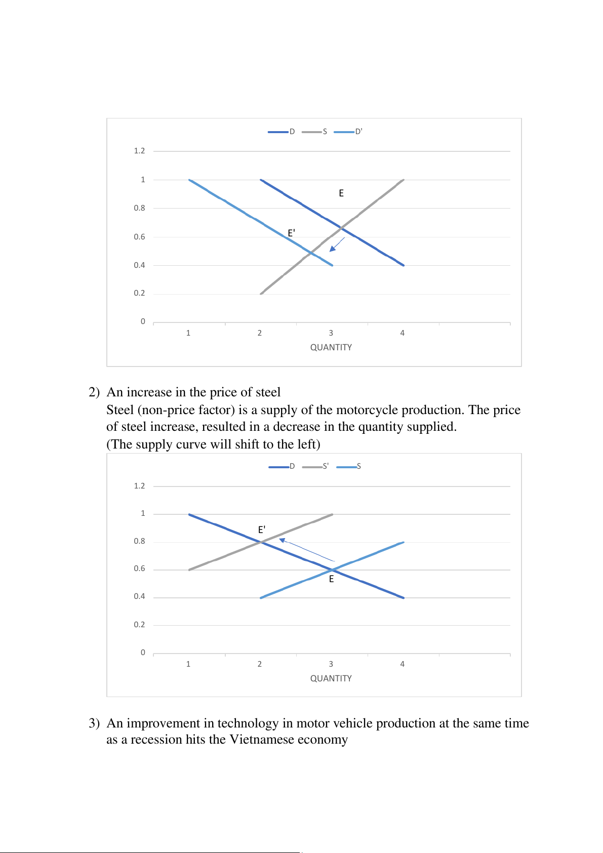
2) An increase in the price of steel
Steel (non-price factor) is a supply of the motorcycle production. The price
of steel increase, resulted in a decrease in the quantity supplied.
(The supply curve will shift to the left) D S' S 1.2 1 E' 0.8 ICE 0.6 R P E 0.4 0.2 0 1 2 3 4 QUANTITY
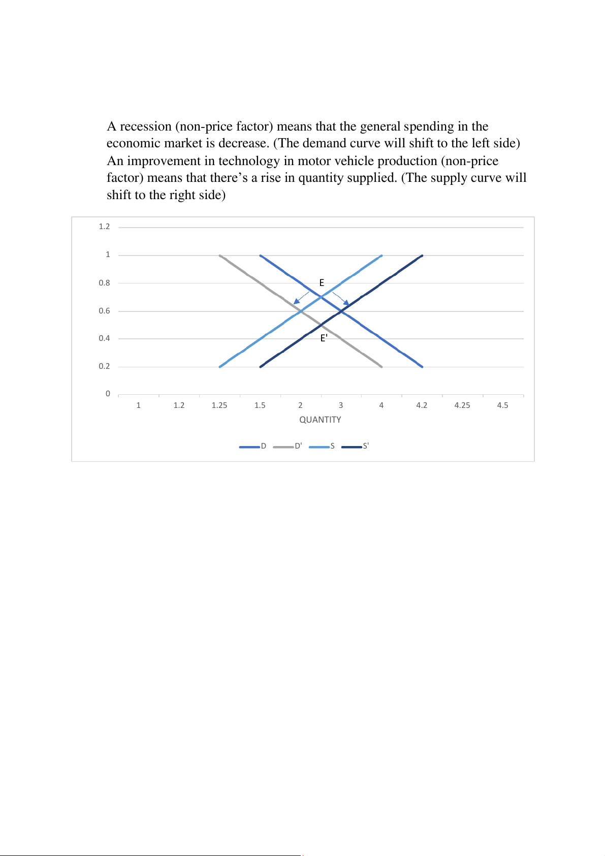
3) An improvement in technology in motor vehicle production at the same time
as a recession hits the Vietnamese economy
A recession (non-price factor) means that the general spending in the
economic market is decrease. (The demand curve will shift to the left side)
An improvement in technology in motor vehicle production (non-price
factor) means that there’s a rise in quantity supplied. (The supply curve will shift to the right side) 1.2 1 0.8 E ICE 0.6 R P 0.4 E' 0.2 0 1 1.2 1.25 1.5 2 3 4 4.2 4.25 4.5 QUANTITY D D' S S'