Lecture 04: Understanding Linear Equations & Functions | Microeconomics | Trường Đại học Quốc tế, Đại học Quốc gia Thành phố Hồ Chí Minh

Lecture 4 QUANTITATIVE LINEAR EQUATIONS METHODS AND LINEAR FUNCTIONS Lecture 4 LEARNING OBJECTIVES Solve linear equations.
Write down the equation of the straight line when given (i) the
value of slope and intercept and (ii) the slope of the line and a point on the line.
Calculate the equilibrium price and quantity in the goods market and the labour market.
Calculate and illustrate graphically break – even, profit and loss. Lecture 4 INTRODUCTION
We have learned arithmetic rules, laws and formulas to simplify the
expressions. Sometimes, it is straightforward to simplify a more
complicated expression, but sometimes it is not.
Equations provide a clear direction for simplifying or transforming
expressions. The ultimate purpose is to solve for the unknown
variable in an equation by making use of the rules, laws and formulas.
Why? It is very rare to know everything you want to know in reality.
Some questions need to be answered by collecting new information
(induction), but many can be answered by pure deduction. Lecture 4 INTRODUCTION
An equation is any mathematical relationship linking different
variables and parameters by operations. It can be a definition (e.g.
, profit equals to total revenue
minus total costs ), a behavioural relationship (e.g. , demand
is negatively depending on price ), or an equilibrium condition (e.g.
, the market clearing condition is supply equals to demand). You need some conventions (accounting) and/or theories
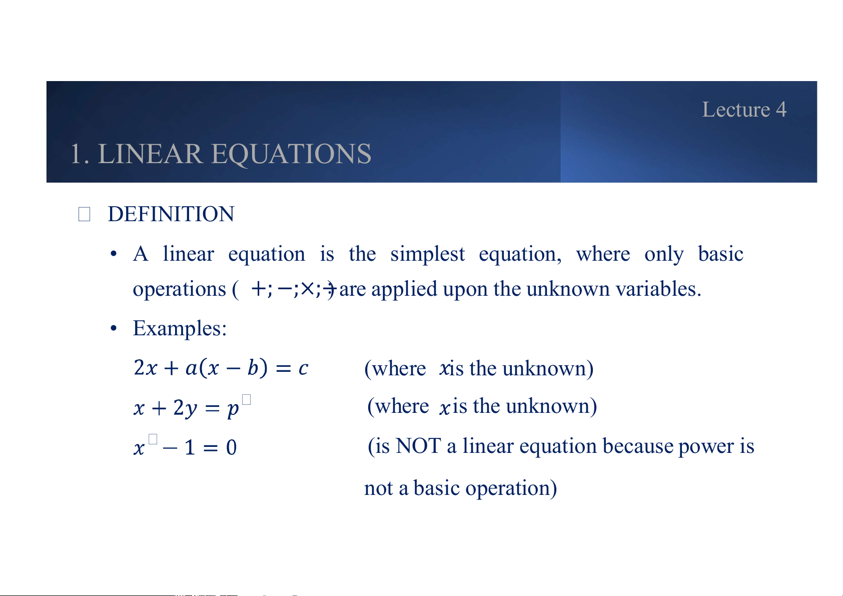
(finance/economic/physics) to formulate an equation. Lecture 4 1. LINEAR EQUATIONS DEFINITION
• A linear equation is the simplest equation, where only basic operations (
) are applied upon the unknown variables. • Examples: (where is the unknown) (where is the unknown)
(is NOT a linear equation because power is not a basic operation) Lecture 4 1. LINEAR EQUATIONS DEFINITION
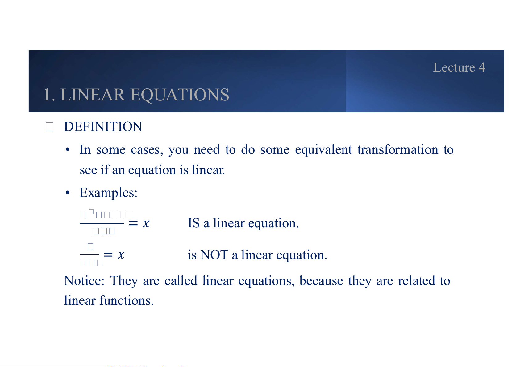
• In some cases, you need to do some equivalent transformation to see if an equation is linear. • Examples: IS a linear equation. is NOT a linear equation.
Notice: They are called linear equations, because they are related to linear functions. Lecture 4 1. LINEAR EQUATIONS SOLVING A LINEAR EQUATION
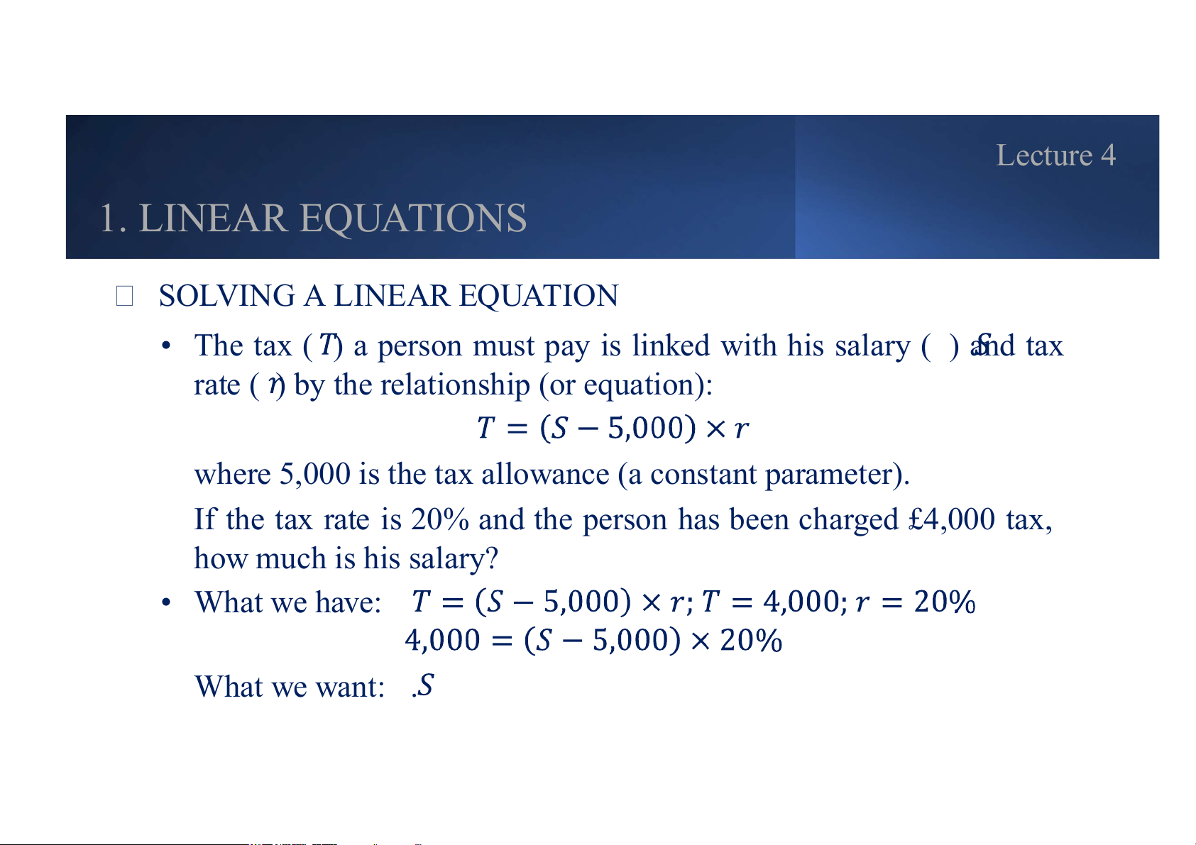
• The tax ( ) a person must pay is linked with his salary ( ) and tax
rate ( ) by the relationship (or equation):
where 5,000 is the tax allowance (a constant parameter).
If the tax rate is 20% and the person has been charged £4,000 tax, how much is his salary? • What we have: . What we want: . Lecture 4 1. LINEAR EQUATIONS SOLVING A LINEAR EQUATION
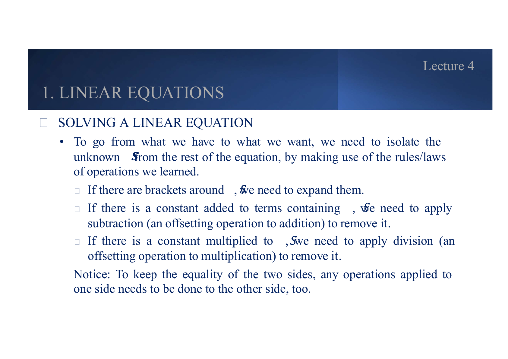
• To go from what we have to what we want, we need to isolate the
unknown from the rest of the equation, by making use of the rules/laws of operations we learned.
If there are brackets around , we need to expand them.
If there is a constant added to terms containing , we need to apply
subtraction (an offsetting operation to addition) to remove it.
If there is a constant multiplied to , we need to apply division (an
offsetting operation to multiplication) to remove it.
Notice: To keep the equality of the two sides, any operations applied to
one side needs to be done to the other side, too. Lecture 4 1. LINEAR EQUATIONS SOLVING A LINEAR EQUATION what we have expand brackets simplify the right-hand side remove on the right-hand
side by applying an offsetting operation on both sides remove on the right-hand side
by applying an offsetting operation on both sides which is equivalent to
, and this is exactly what we want. Lecture 4 1. LINEAR EQUATIONS
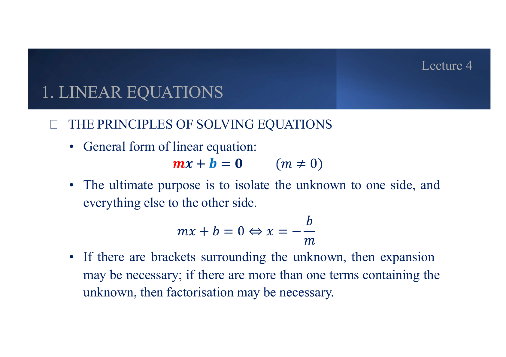
THE PRINCIPLES OF SOLVING EQUATIONS
• General form of linear equation:
• The ultimate purpose is to isolate the unknown to one side, and
everything else to the other side.
• If there are brackets surrounding the unknown, then expansion
may be necessary; if there are more than one terms containing the
unknown, then factorisation may be necessary. Lecture 4 1. LINEAR EQUATIONS
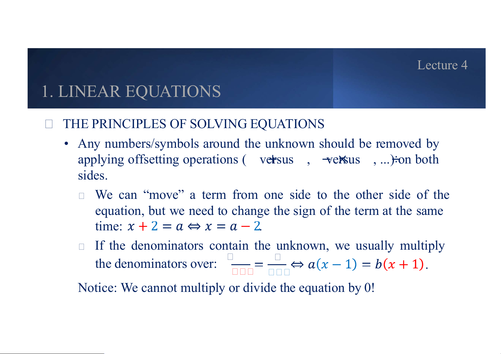
THE PRINCIPLES OF SOLVING EQUATIONS
• Any numbers/symbols around the unknown should be removed by
applying offsetting operations ( versus , versus , ...) on both sides.
We can “move” a term from one side to the other side of the
equation, but we need to change the sign of the term at the same time: .
If the denominators contain the unknown, we usually multiply the denominators over: .
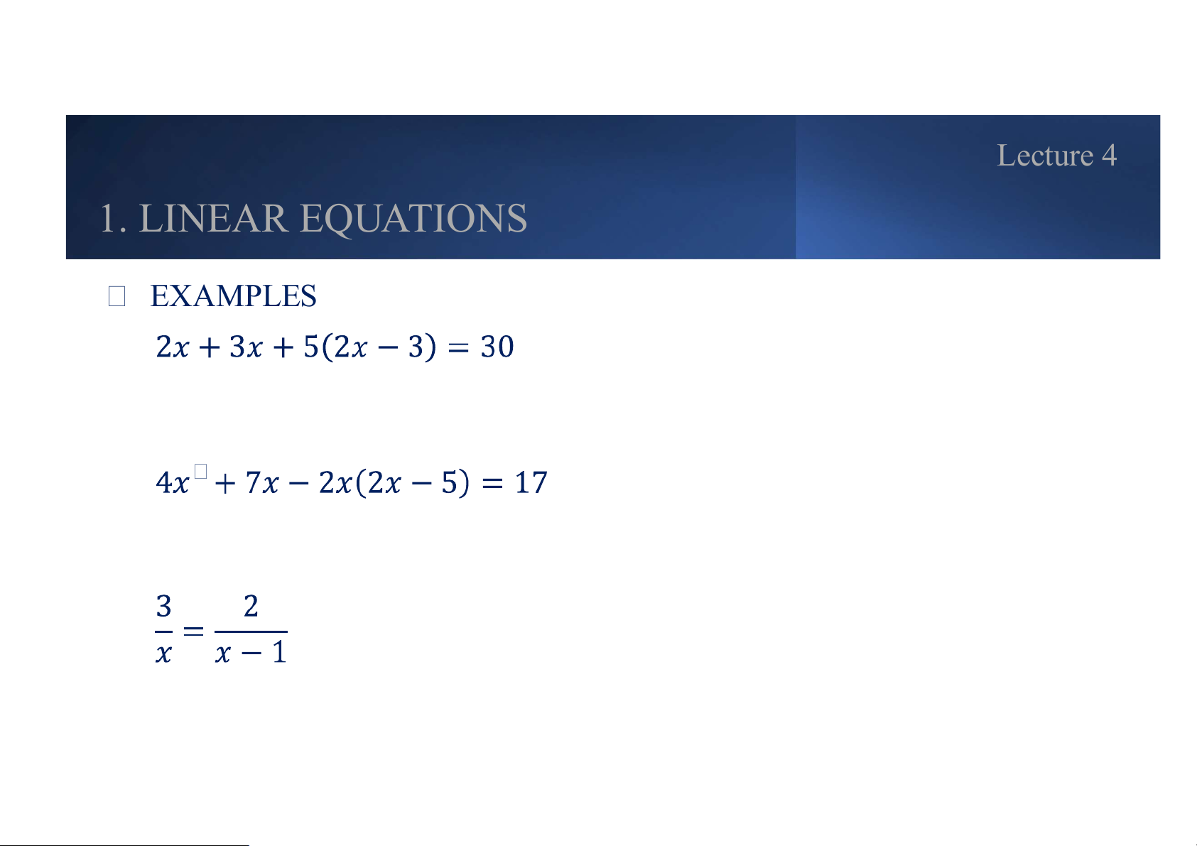
Notice: We cannot multiply or divide the equation by 0! Lecture 4 1. LINEAR EQUATIONS EXAMPLES Lecture 4 2. LINEAR FUNCTIONS THE SLOPE – INTERCEPT FORM
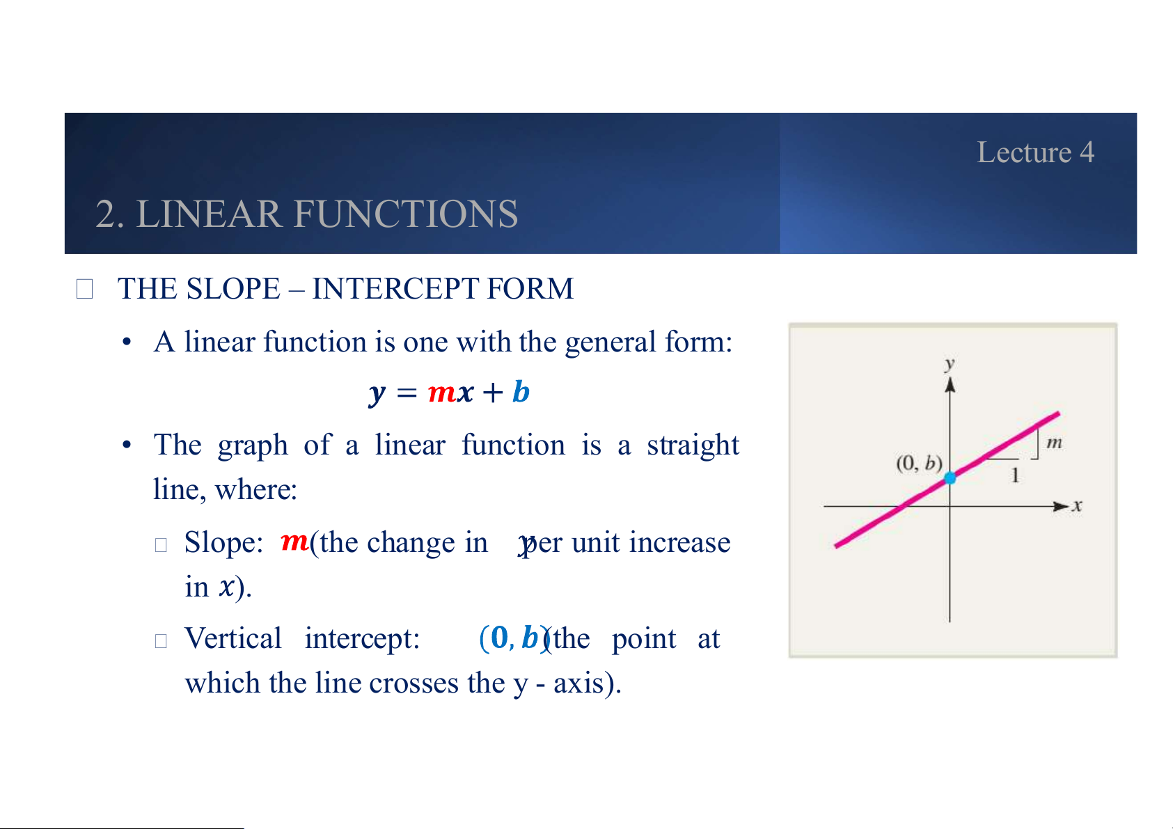
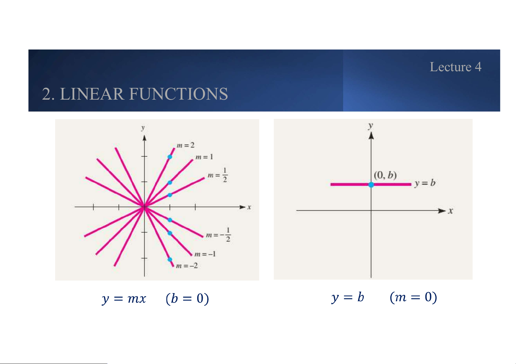
• A linear function is one with the general form:
• The graph of a linear function is a straight line, where: Slope:
(the change in per unit increase in ). Vertical intercept: (the point at
which the line crosses the y - axis). Lecture 4 2. LINEAR FUNCTIONS Lecture 4 2. LINEAR FUNCTIONS GRAPHIC
• To sketch a linear function by hand, we only need two points
(because any two points can fix a unique line).
• For convenience, we usually choose the two special points cutting at the two axes, that is: When ,
(the intercept on vertical axis). When ,
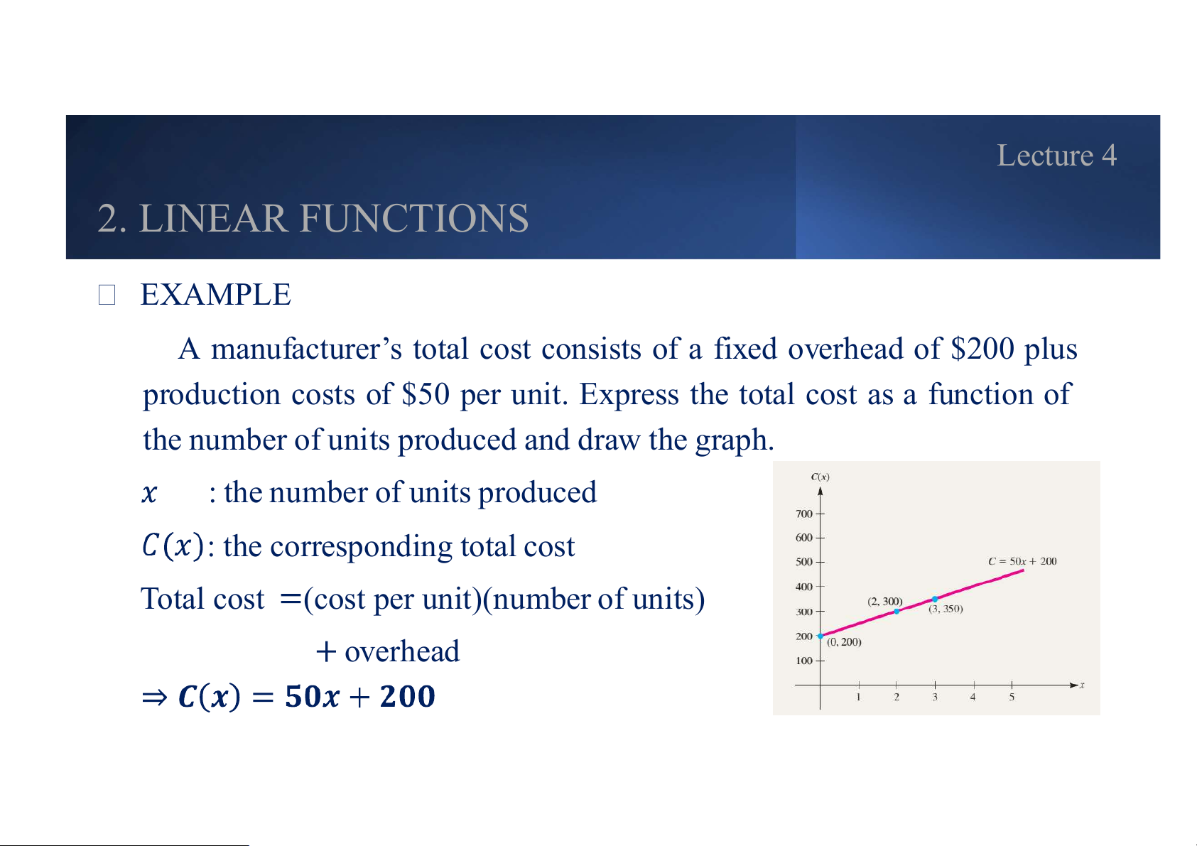
(the intercept on horizontal axis). Lecture 4 2. LINEAR FUNCTIONS EXAMPLE
A manufacturer’s total cost consists of a fixed overhead of $200 plus
production costs of $50 per unit. Express the total cost as a function of
the number of units produced and draw the graph. : the number of units produced : the corresponding total cost
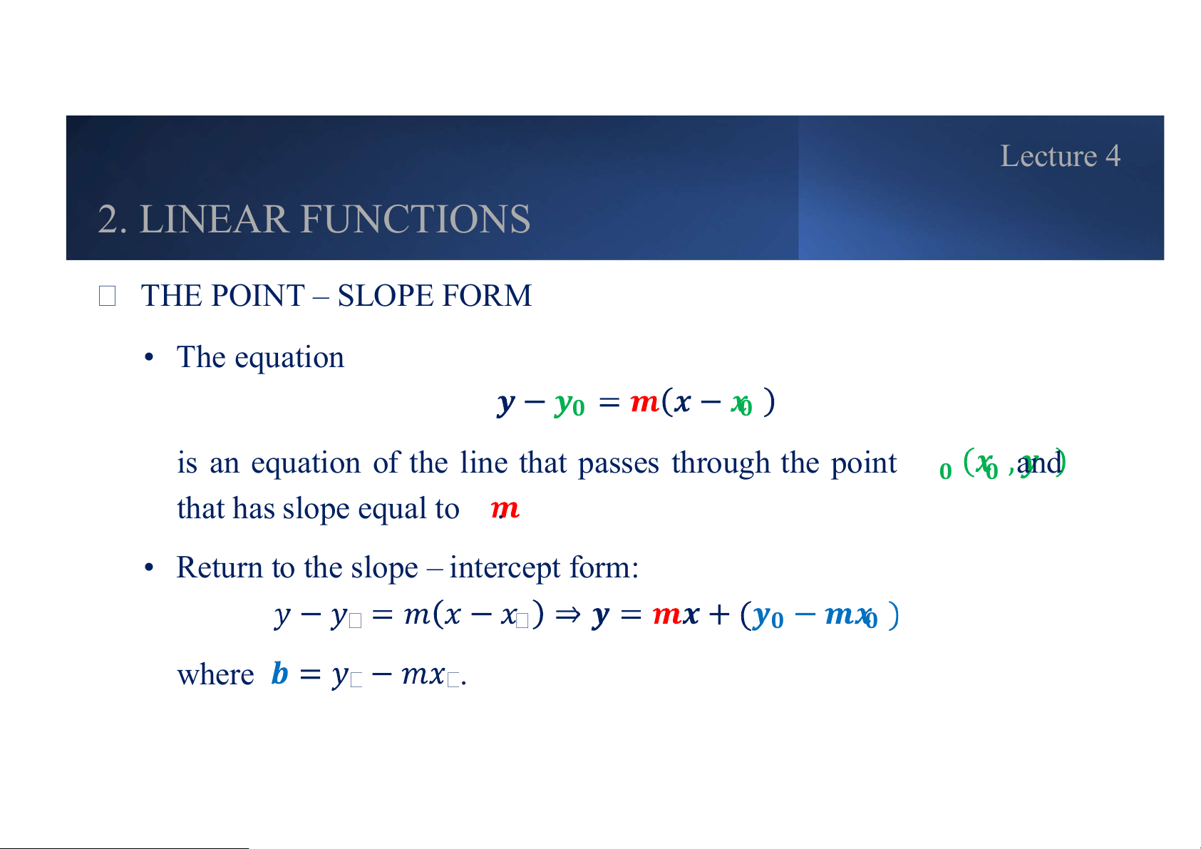
Total cost (cost per unit)(number of units) overhead Lecture 4 2. LINEAR FUNCTIONS THE POINT – SLOPE FORM • The equation 𝟎 𝟎
is an equation of the line that passes through the point 𝟎 𝟎 and that has slope equal to .
• Return to the slope – intercept form: 𝟎 𝟎 where . Lecture 4 2. LINEAR FUNCTIONS EXAMPLE
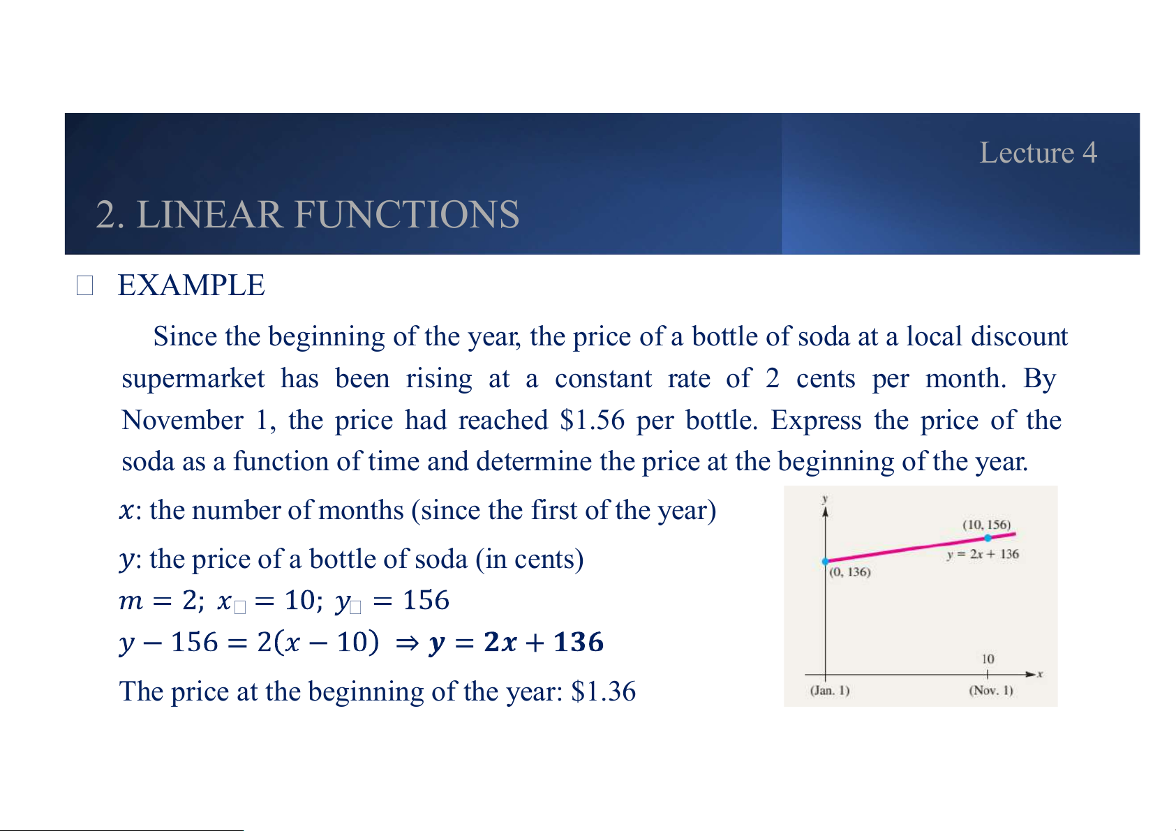
Since the beginning of the year, the price of a bottle of soda at a local discount
supermarket has been rising at a constant rate of 2 cents per month. By
November 1, the price had reached $1.56 per bottle. Express the price of the
soda as a function of time and determine the price at the beginning of the year.
: the number of months (since the first of the year)
: the price of a bottle of soda (in cents)
The price at the beginning of the year: $1.36 Lecture 4 2. LINEAR FUNCTIONS
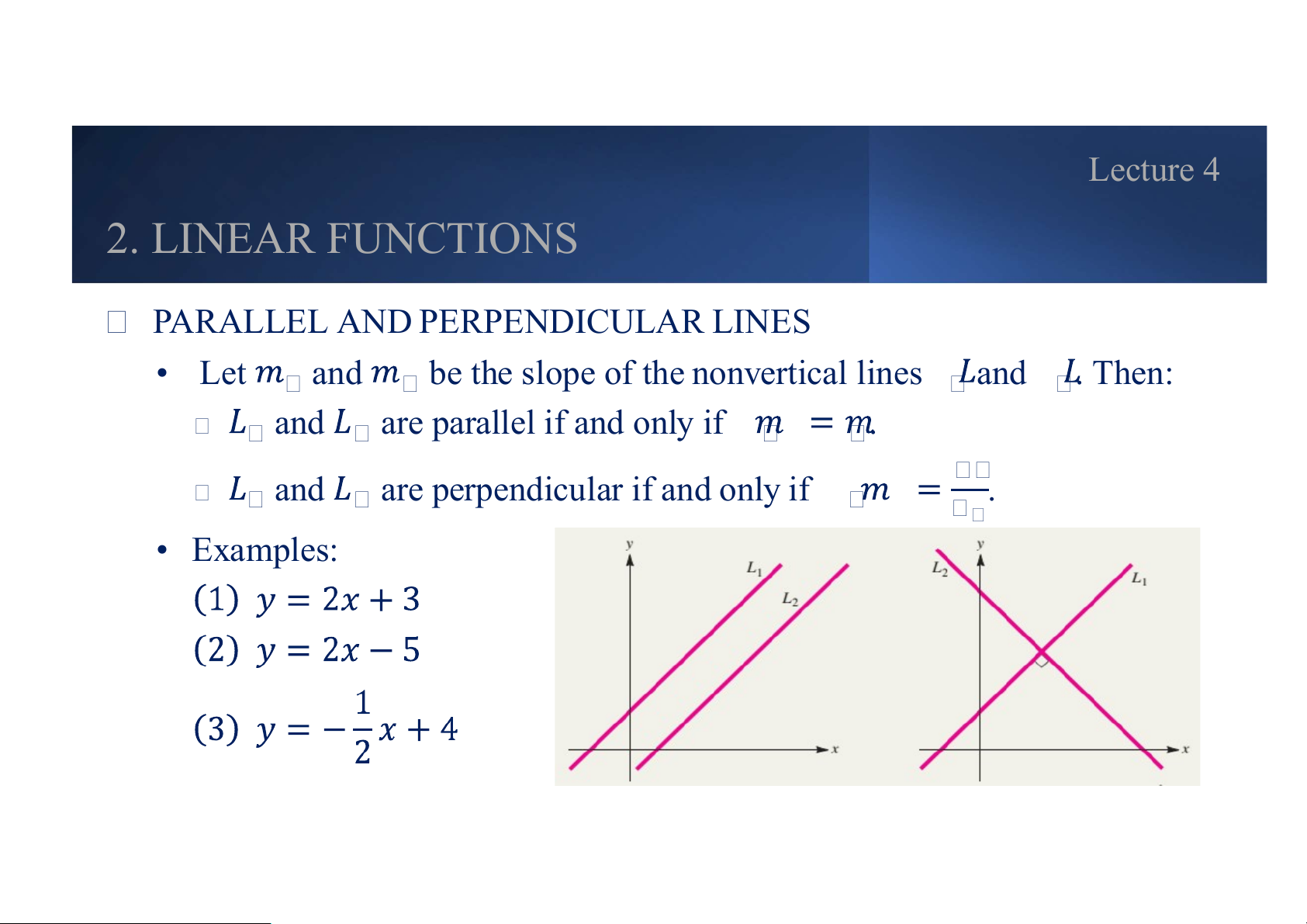
PARALLEL AND PERPENDICULAR LINES • Let and
be the slope of the nonvertical lines and . Then: and are parallel if and only if . and
are perpendicular if and only if . • Examples: Lecture 4 2. LINEAR FUNCTIONS
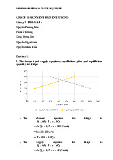
APPLICATION: GOOD MARKET EQUILIBRIUM
• Good market equilibrium occurs when the quantity demanded by
consumers and the quantity supplied by producers of a good or service are equal.
• Equivalently, market equilibrium occurs when the price that a consumer is willing to pay
is equal to the price that a producer is willing to accept .