Lý thuyết xác suất - Toán Kinh Tế | Đại học Tôn Đức Thắng

LÝ THUYẾT XÁC SUẤT
Random variables and distributions 1. Random variables
A function X: (Omega, F ) -> (R, Borel) satisfying
X^-1(B) in F, for all B in Borel
X^-1(B) = {w in Omega: X(w) in B} con của Omega Example: X: Omega -> R w -> X(w) X(w) = 1 if w in A 0 if w notin A Take B in Borel
X^-1(B) = {w in Omega: X (w) in B} = Omega if 0 in B and 1 in B Rỗng if 0 notin B and 1 notin B A if 0 notin B and 1 in B Ac if 0 in B and 1 notin B  X^-1(B) in F  X is r.v’.s Problem 2.1 Trình bày như bài trên Problem 2.2: Take B in Borel. Let X(w) = a
X^-1(B) = {w in Omega: X (w) in B} = Omega if a in B Rỗng if a notin B  X^-1 (B) in F  X is r.v’.s Example: Omega:= {HH, HT, TH, TT} Define: X: Omega -> R X(HH) = 2 X(HT) = X(TH) = 1 X(TT) = 0 . F = 2^Omega Take B in Borel
X^-1(B) = {w in Omega: X (w) in B} con Omega  X^-1(B) in F  X is a r.v
. F = {Omega, Rỗng, {HH, HT}, {TH, TT}}
Take B0 = {0} in B (= [0, +inf) cap (-inf, 0])
X^-1(B0) = {w in Omega: X(w) = 0} = {TT} notin F  X is not r.v
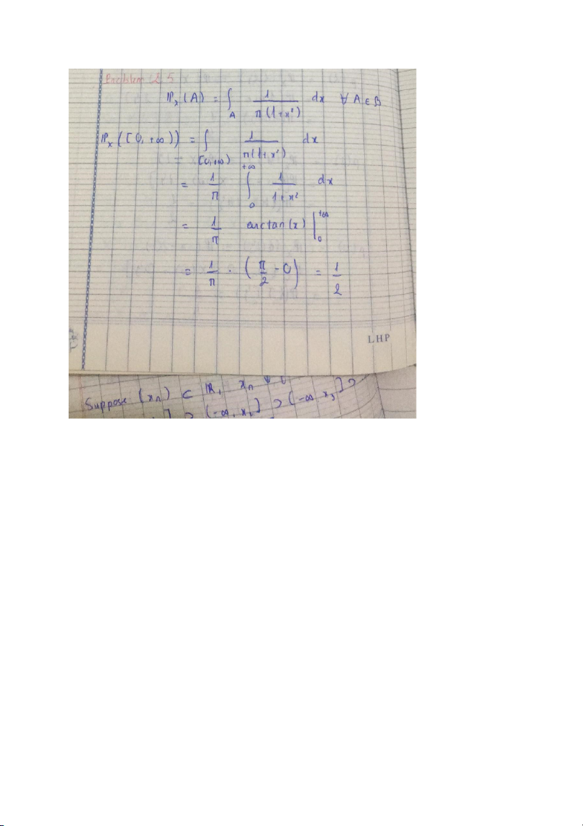
Definition (Distribution): Let X: (Omega, F, P) -> (R, Borel) be a r.v Define: Px: Borel -> R B -> Px(B) Px(B) = P[X^-1(B)]
Then Px(B) is called the distribution of X (law of X)
Theorem: Px is a probability measure on Borel
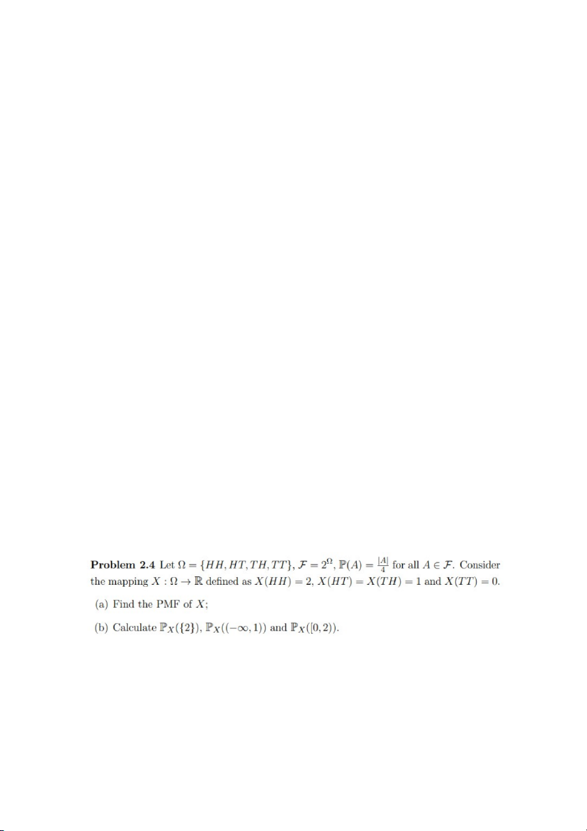
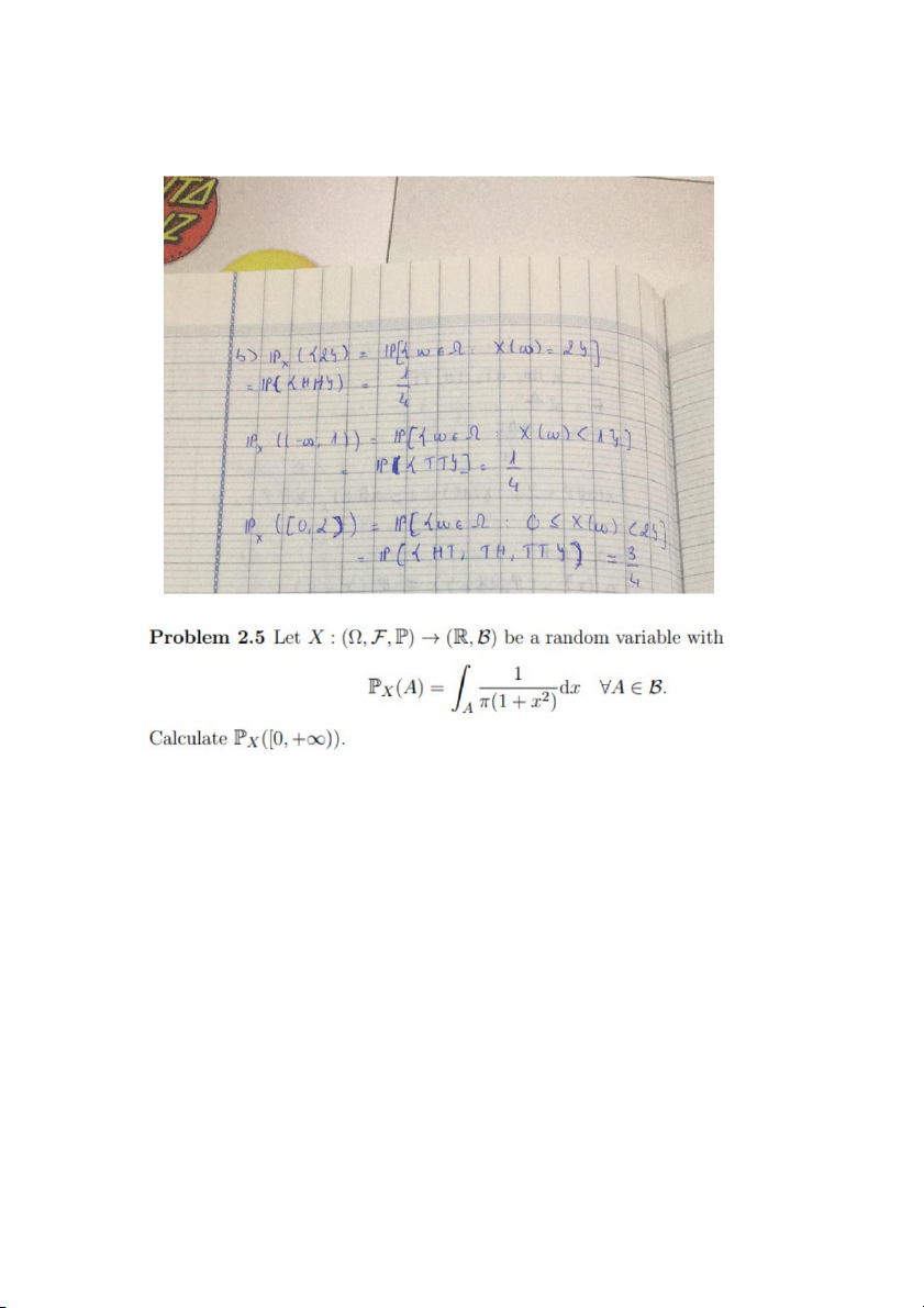
Example: Omega:= {HH, HT, TH, TT} F = 2^Omega P(A) = |A| / |Omega| X(HH) = 2 X(HT) = X(TH) = 1 X(TT) = 0 Find Px((0,+inf)) and Px({2})
. Px((0,+inf)) = P(X^-1((0,+inf))) = P({w in Omega: X(w) > 0}) = P({HH, HT, TH}) = ¾ . Px({2}) = P(X^-1({2})) = P({w in Omega: X(w) = 2}) =P({HH}) = ¼
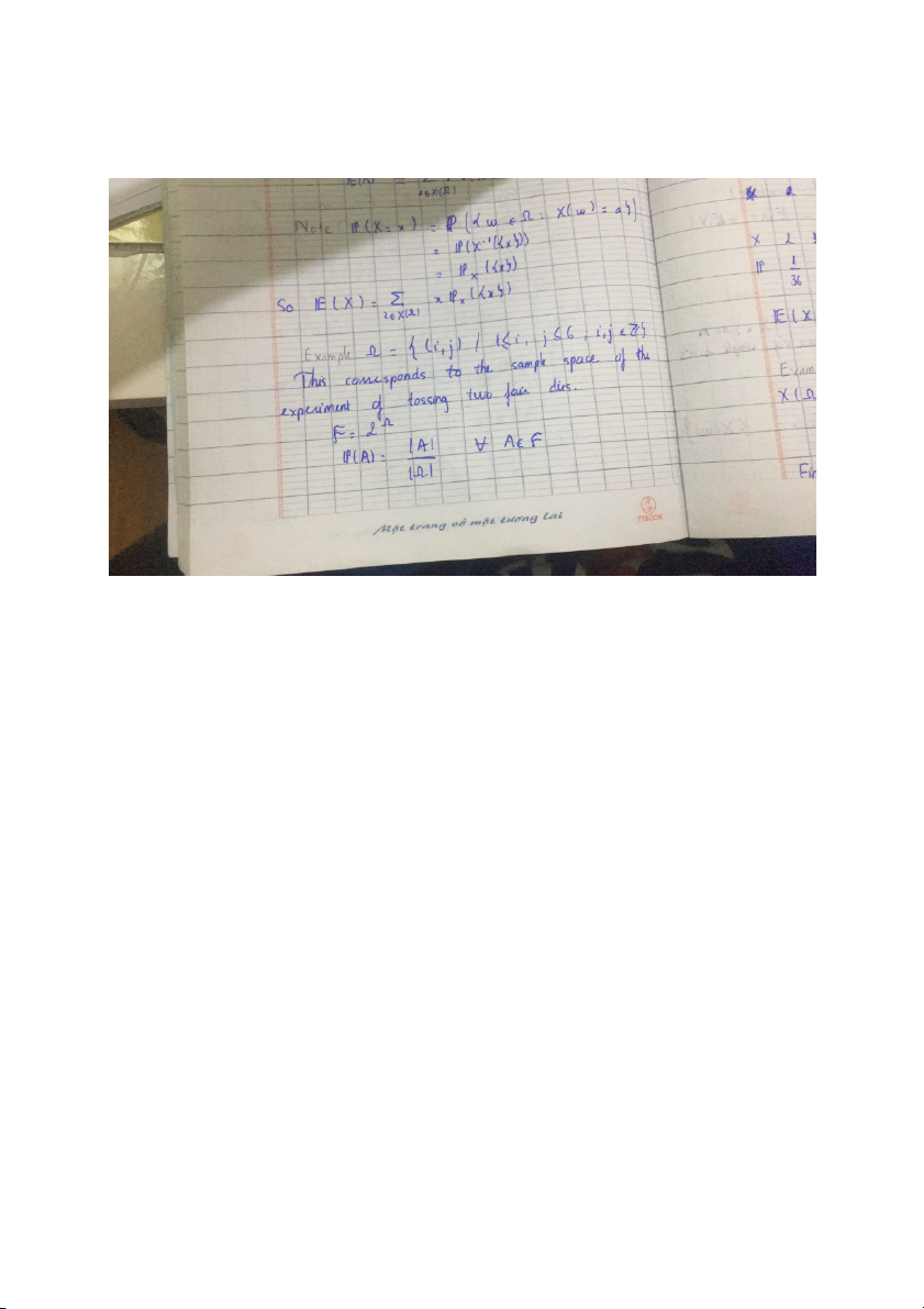
Note: Px(B) = P(X^-1(B)) = P({w in Omega: X(w) in B}) = P({x in B}) =|{w in Omega: X(w) in B}|/4 = |{x in B}|/4 Definition; Two r.v X and Y Px = Py
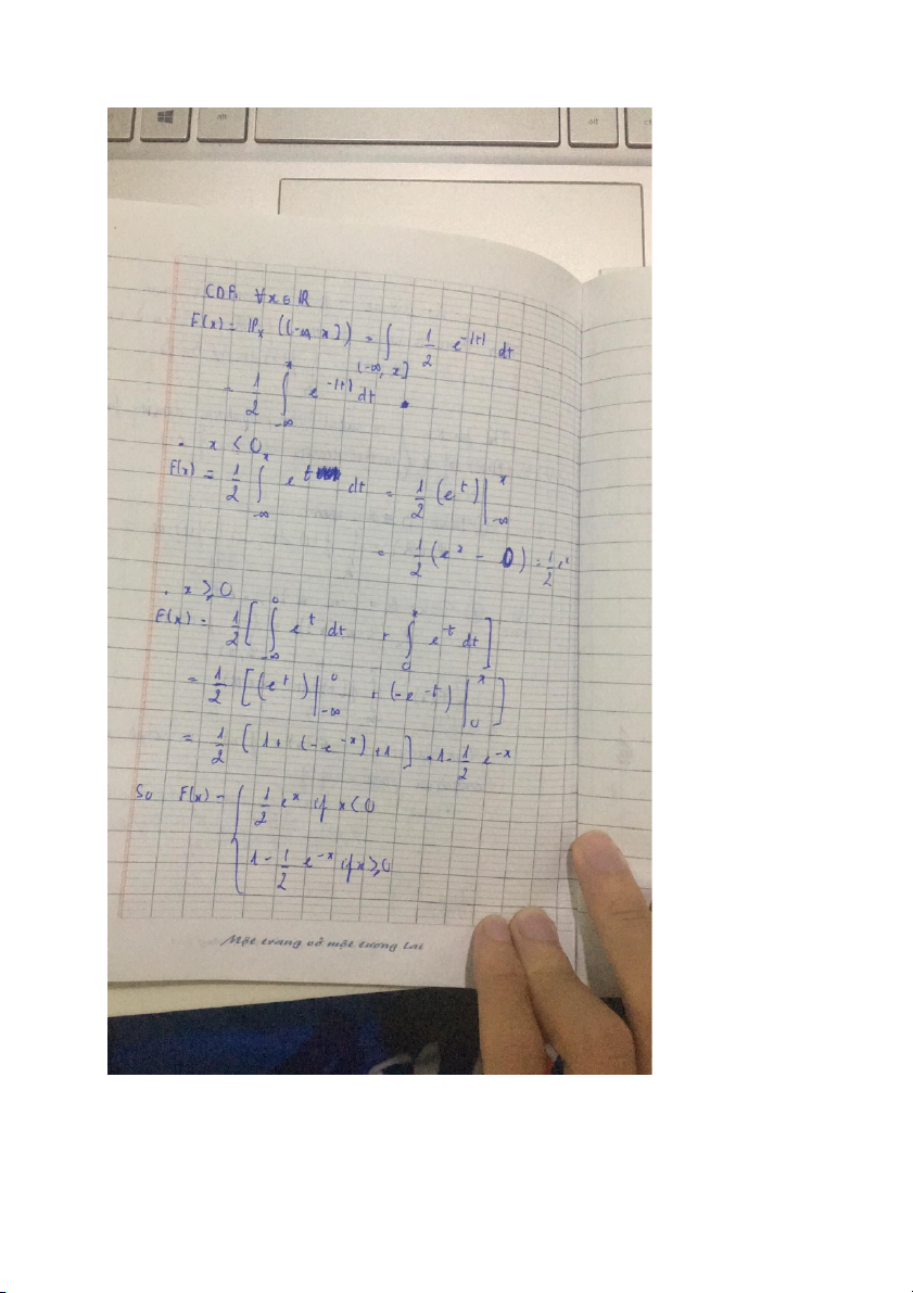
For all B in Borel, Px(B) = Py(B) Definition: (CDF) F(x) F: R -> R x -> F(x) = Px((-inf,x])
F(x) = Px((-inf,x]) = P(X^-1((-inf,x])) = P({w in Omega: X(w) <= x}) = P({X<=x}) = P(X<=x)
Example: Omega:= {HH, HT, TH, TT} F = 2^Omega P(A) = |A| / |Omega| X(HH) = 2 X(HT) = X(TH) = 1 X(TT) = 0 F(x) = P(X<=x) = P(Ax)
. x < 0: Ax = Rỗng => P(Ax) = 0
.0<= x < 1: Ax = {TT} => P(Ax) = ¼
. 1<= x < 2: Ax = {TT, HT, TH}=> P(Ax) = ¾
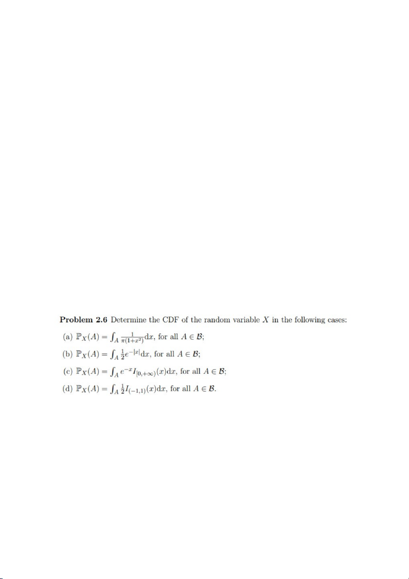
. x>=2 : Ax = Omega => P(Ax) =1 So F(x) = 0 if x < 0 ¼ if 0<=x<1 ¾ if 1<=x<2 1 if x >= 2 Problem 2.6: c) I[0,+inf) (x) = 1 if x in [0, +inf) 0 if x notin [0, +inf)
F(x) = Px((-inf, x]) = tp(-inf, x] e^-x . I[0,+inf) (x)dx .x < 0:
F(x) = tp(-inf -> x) 0 dx = 0 .x >=0:
F(x) = tp(-inf -> x) e^-x dx = tp(-inf -> 0) 0 dx + tp(0 -> x)e^-x dx = -e^-x + 1 d) I(-1,1) = 1 if x in (-1,1) 0 if x not in (-1,1)
F(x) = P(X^-1(-inf,x]) = ½ tp(-inf,x] I(-1,1)(x) dx . x < -1 ½ tp(-inf -> x) 0 dx = 0
.-1½ tp(-inf -> -1 ) 0 dx + ½ tp(-1 -> x) dx = ½(x+1) . x > 1
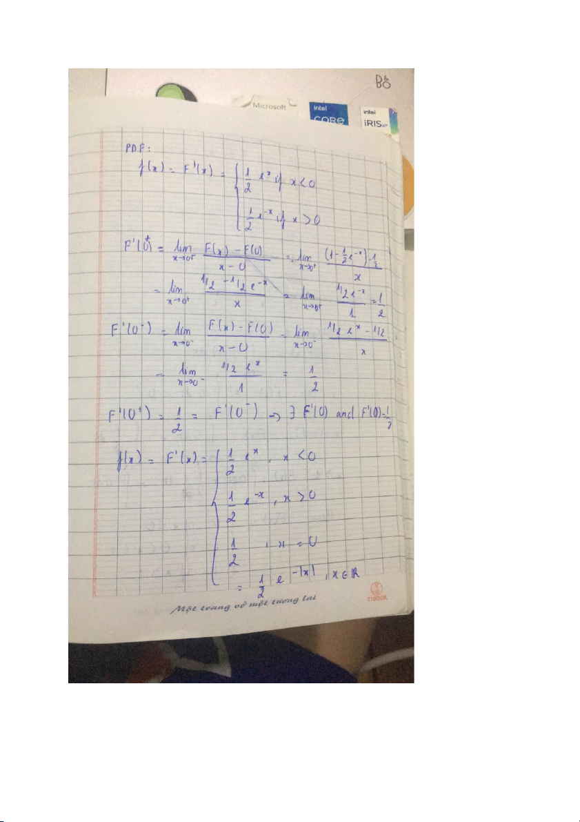
½ tp(-inf -> -1 ) 0 dx + ½ tp(-1 -> 1) dx + ½ tp(1->x) 0 dx = 1 Definition: PMF p(x) = P_X ({x}) = P(X = x) Theorem: P_X(B) = tpB f(t) dt f is (PDF) F’(x) = f(x) F(x) = tp(-inf,x] f(t) dt
a) p(x) = P_X({x}) = P({w in Omega: X(w) = x}) . x = Omega
p(x) = P_X({x}) = P({w in Omega: X(w) = Omega}) = 1 b)
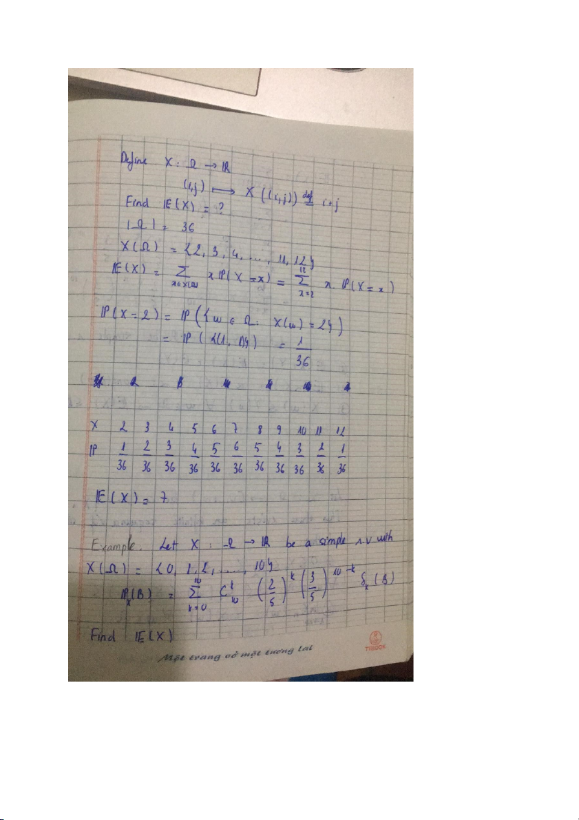
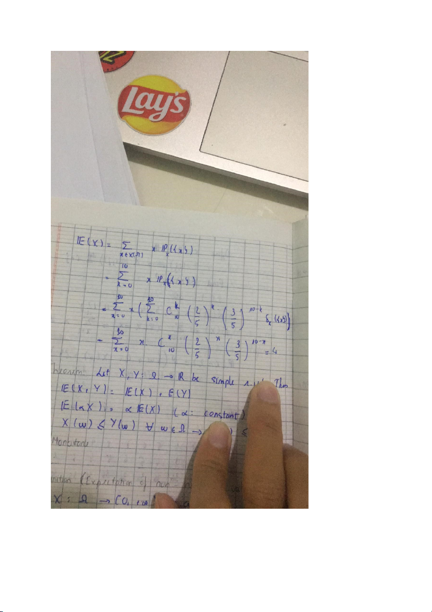
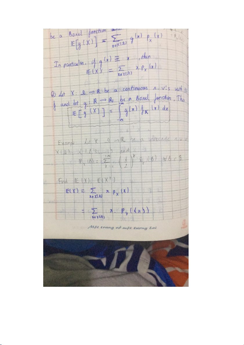
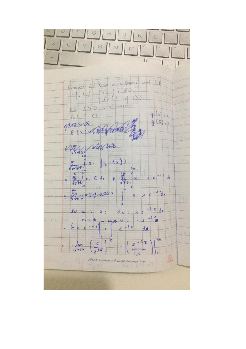
E(x) = Sigma xP(X=x) = sigma x P_X({x}) Lazy Statistician 1. E[g(X)] = sigma g(x)p_X (x)
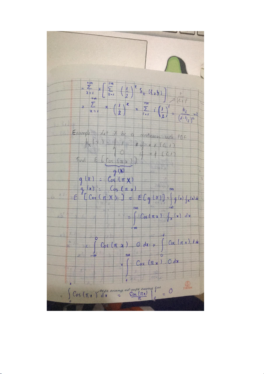
If g(x) = x => E(X) = sigma x.p_X (x)
2. E[g(X)] = tp (-inf, + inf) g(x)f_X(x) dx With PDF Var
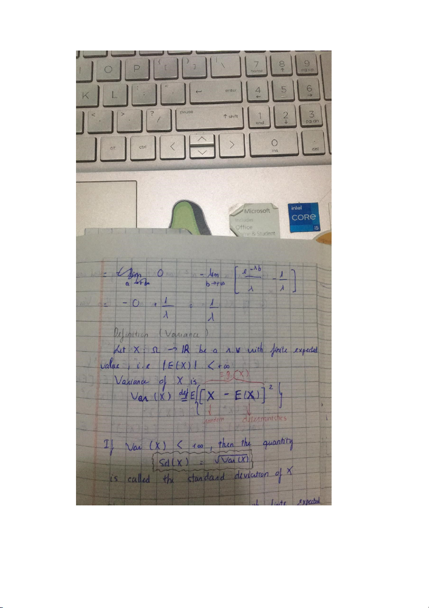
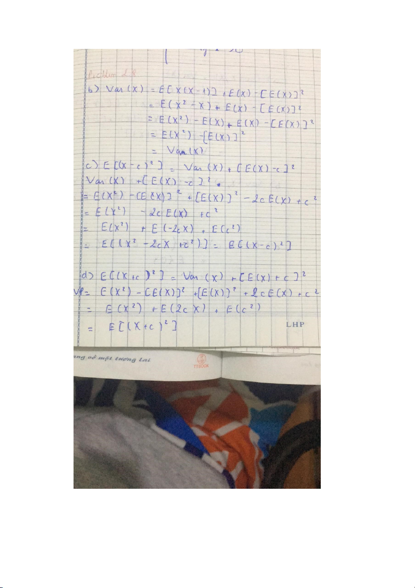
Var(X) = E(X^2) – [E(X)]^2 Sd = sqrt(Var(X)) Cov
Cov(X) = E{[X – E(X)][Y – E(Y)]}
p(X, Y) = Cov / sqrt( Var(X).Var(Y))