Microeconomics Presentation Assignment 3 | Microeconomics | Trường Đại học Quốc tế, Đại học Quốc gia Thành phố Hồ Chí Minh
Tài liệu được sưu tầm và soạn thảo dưới dạng file PDF với mục đích hỗ trợ học tập và tham khảo. Nội dung tài liệu được trình bày rõ ràng, dễ tiếp cận, phù hợp cho việc ôn tập và củng cố kiến thức trong quá trình học đại học. Đây sẽ là nguồn tư liệu hữu ích giúp các bạn sinh viên chuẩn bị tốt hơn cho các buổi học, đồng thời mở rộng thêm hiểu biết về môn học. Hy vọng tài liệu này sẽ mang lại nhiều giá trị và hỗ trợ các bạn trong hành trình học tập. Mời bạn đọc cùng tham khảo!
Môn: Microeconomics 635 tài liệu
Trường: Trường Đại học Quốc tế, Đại học Quốc gia Thành phố Hồ Chí Minh 1.9 K tài liệu
Tác giả:


Preview text:
LE BICH NGOC - 11230122 CLASS: EBBA 15.2 PRESENTATION ASSIGNMENT 3 1. Case 1
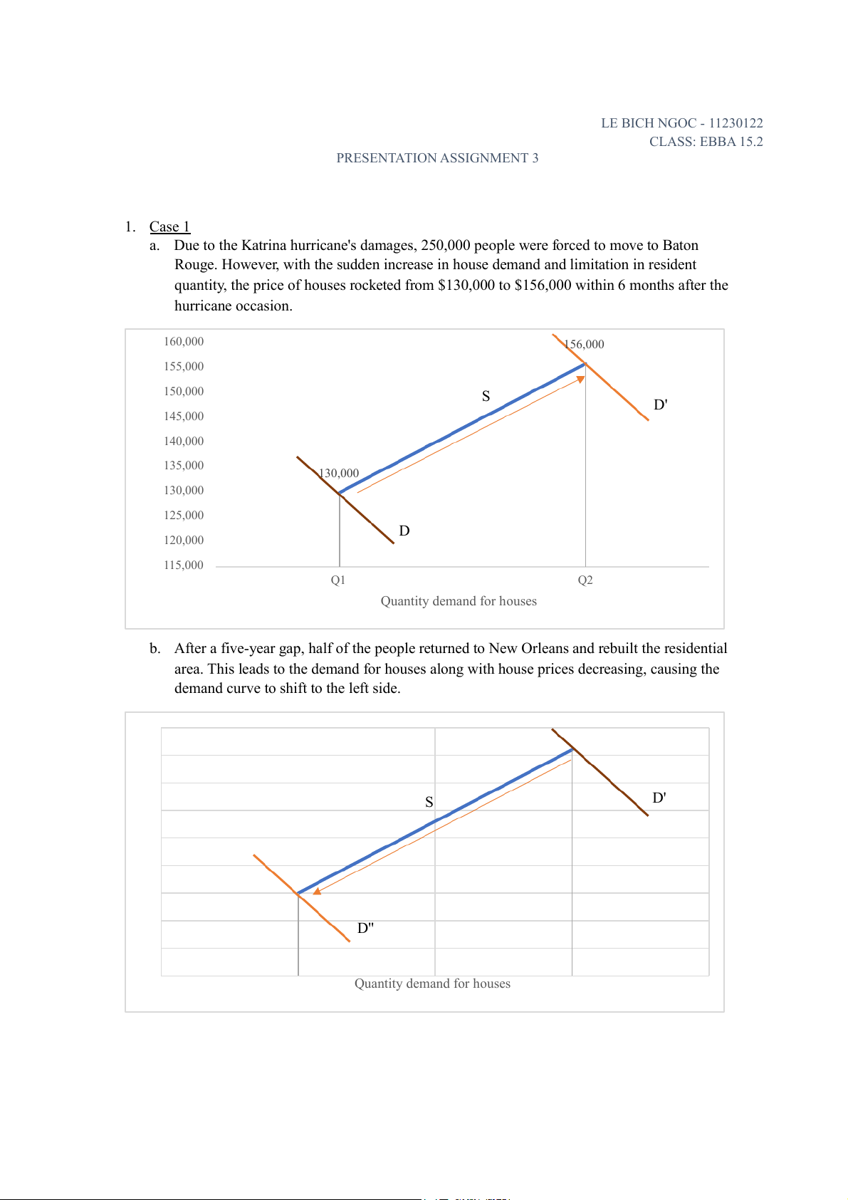
a. Due to the Katrina hurricane's damages, 250,000 people were forced to move to Baton
Rouge. However, with the sudden increase in house demand and limitation in resident
quantity, the price of houses rocketed from $130,000 to $156,000 within 6 months after the hurricane occasion. 160,000 156,000 155,000 150,000 S D' 145,000 140,000 135,000 ouse price 130,000 H 130,000 125,000 D 120,000 115,000 Q1 Q2 Quantity demand for houses
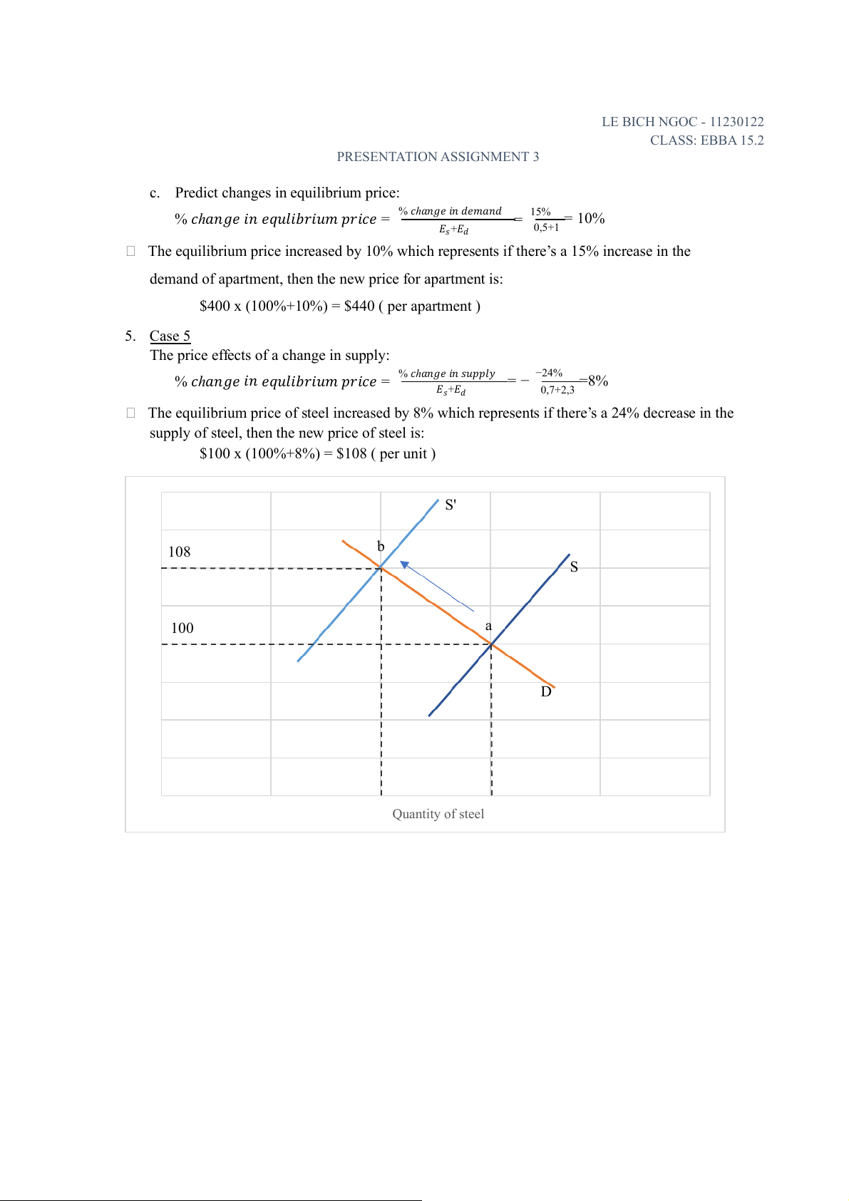
b. After a five-year gap, half of the people returned to New Orleans and rebuilt the residential
area. This leads to the demand for houses along with house prices decreasing, causing the
demand curve to shift to the left side. D' S ouse price H D' Quantity demand for houses LE BICH NGOC - 11230122 CLASS: EBBA 15.2 PRESENTATION ASSIGNMENT 3 2. Case 2
Due to the occasion of bee colony collapse disorder (CCD), pollination dropped, leading
to the production of a wide variety of fruits, vegetables, and nuts also decreased. Th e
supplement for ice cream (berries and nuts) witnessed a shortage, causing the supply curve to shift to the left.
Since the price of producing ice cream increased, it pushed the price of ice cream to be
higher. Based on the scenario, it is expected that the demand for ice cream to drop, making the
demand curve shift to the left. S' S P2 price P1 D Ice cream D' B1 B2 Bee population 3. Case 3
a. Calculation for the elasticity of demand: Quantity Price Initial
𝑄1 = 1 𝑚𝑒𝑎𝑙/𝑚𝑜𝑛𝑡ℎ $10/person After the voucher
𝑄2 = 3 𝑚𝑒𝑎𝑙/𝑚𝑜𝑛𝑡ℎ $5/person Percentage change ∆𝑄 2 ∆𝑃 −5 %∆𝑄 . 100% . 100% 𝑑 = . 100% = %∆𝑃 = . 100% = 𝑄1 1 𝑃 10 = 200% = −50% Elasticity of demand 𝐸 𝑑
| = |200% | = 4 > 1 => elastic 𝑝 = |%∆𝑄𝑑 %∆𝑃 −50%
b. After giving out the voucher to Mr. and Mrs. Binh – providing two meals for the price of one,
it encouraged them to dine out more often, which increases Binh’s monthly expenditure on meals at this restaurant.
The change in total expenditure remains consistent with the value of demand ( 𝐸 𝑑 𝑝 > 1 ). LE BICH NGOC - 11230122 CLASS: EBBA 15.2 PRESENTATION ASSIGNMENT 3 4. Case 4
Consider a college town where the initial price of rental apartments is $400 and the initial
quantity is 1,000 apartments. The price elasticity of demand for apartments is 1.0 and the price
elasticity of sully of apartments is 0.5.
a. Use demand and supply curves to show the initial equilibrium, and label the equilibrium point a. 700 600 500 a 400 PRICE 300 200 100 0 0 2 0 0 4 0 0 6 0 0 8 0 0 1 0 0 0 1 2 0 0 1 4 0 0 1 6 0 0 1 8 0 0 2 0 0 0 APPARTMENT QUANTITY
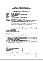
b. Suppose that an increase in college enrollment is expected to increase the demand for
apartments in college town by 15 percent. Use your graph to show the effects of the increase
in demand on the apartments market. Label the new equilibrium point b.
The new quantity demand of apartment: 1000 x (100% +15%) = 1150 (apartment) S b a 400 D' PRICE D 1000 1150 APPARTMENT QUANTITY LE BICH NGOC - 11230122 CLASS: EBBA 15.2 PRESENTATION ASSIGNMENT 3
c. Predict changes in equilibrium price: %
% 𝑐ℎ𝑎𝑛𝑔𝑒 𝑖 𝑛 𝑑𝑒𝑚𝑎𝑛𝑑 𝑐ℎ𝑎𝑛𝑔𝑒 𝑖
𝑛 𝑒𝑞𝑢𝑙𝑖𝑏𝑟𝑖𝑢𝑚 𝑝𝑟𝑖𝑐𝑒 = = 15% = 10% 𝐸 0,5+1 𝑠+𝐸𝑑
The equilibrium price increased by 10% which represents if there’s a 15% increase in the
demand of apartment, then the new price for apartment is:
$400 x (100%+10%) = $440 ( per apartment ) 5. Case 5
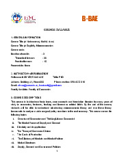
The price effects of a change in supply: %
% 𝑐ℎ𝑎𝑛𝑔𝑒 𝑖 𝑛 𝑠𝑢𝑝𝑝𝑙𝑦 𝑐ℎ𝑎𝑛𝑔𝑒 𝑖
𝑛 𝑒𝑞𝑢𝑙𝑖𝑏𝑟𝑖𝑢𝑚 𝑝𝑟𝑖𝑐𝑒 = = − −24% =8% 𝐸𝑠+𝐸𝑑 0,7+2,3
The equilibrium price of steel increased by 8% which represents if there’s a 24% decrease in the
supply of steel, then the new price of steel is:
$100 x (100%+8%) = $108 ( per unit ) S' b 108 S rice P 100 a D Quantity of steel
Tài liệu liên quan:
-

Chương 3: độ co giãn và các nhân tố ảnh hưởng | Microeconomics | Trường Đại học Quốc tế, Đại học Quốc gia Thành phố Hồ Chí Minh
4 2 -
Microeconomics Syllabus | Microeconomics | Trường Đại học Quốc tế, Đại học Quốc gia Thành phố Hồ Chí Minh
4 2 -
Microeconomics Course Syllabus & Assessment Details | Microeconomics | Trường Đại học Quốc tế, Đại học Quốc gia Thành phố Hồ Chí Minh
4 2 -
Assignment 3 - Elasticity MCQs and Key Concepts | Microeconomics | Trường Đại học Quốc tế, Đại học Quốc gia Thành phố Hồ Chí Minh
4 2 -
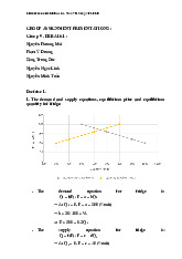
Assignment 2 - Economic Equilibrium Analysis of Fridges and Motorcycles | Microeconomics | Trường Đại học Quốc tế, Đại học Quốc gia Thành phố Hồ Chí Minh
4 2