Production and Cost Analysis in Microeconomics | Microeconomics | Trường Đại học Quốc tế, Đại học Quốc gia Thành phố Hồ Chí Minh

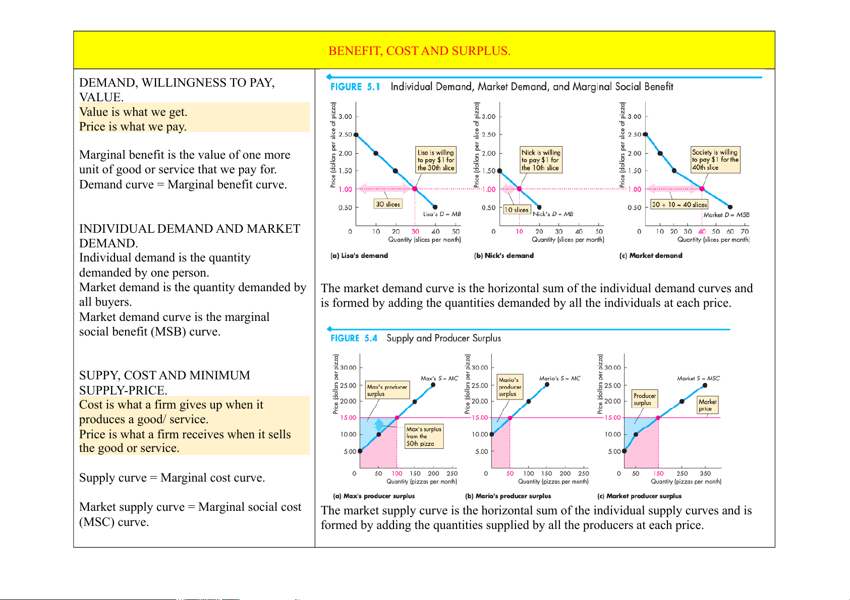
BENEFIT, COST AND SURPLUS. DEMAND, WILLINGNESS TO PAY, VALUE. Value is what we get. Price is what we pay.
Marginal benefit is the value of one more
unit of good or service that we pay for.
Demand curve = Marginal benefit curve. INDIVIDUAL DEMAND AND MARKET DEMAND.
Individual demand is the quantity demanded by one person.
Market demand is the quantity demanded by The market demand curve is the horizontal sum of the individual demand curves and all buyers.
is formed by adding the quantities demanded by all the individuals at each price.
Market demand curve is the marginal social benefit (MSB) curve. SUPPY, COST AND MINIMUM SUPPLY-PRICE.
Cost is what a firm gives up when it produces a good/ service.
Price is what a firm receives when it sells the good or service.
Supply curve = Marginal cost curve.
Market supply curve = Marginal social cost
The market supply curve is the horizontal sum of the individual supply curves and is (MSC) curve.
formed by adding the quantities supplied by all the producers at each price.
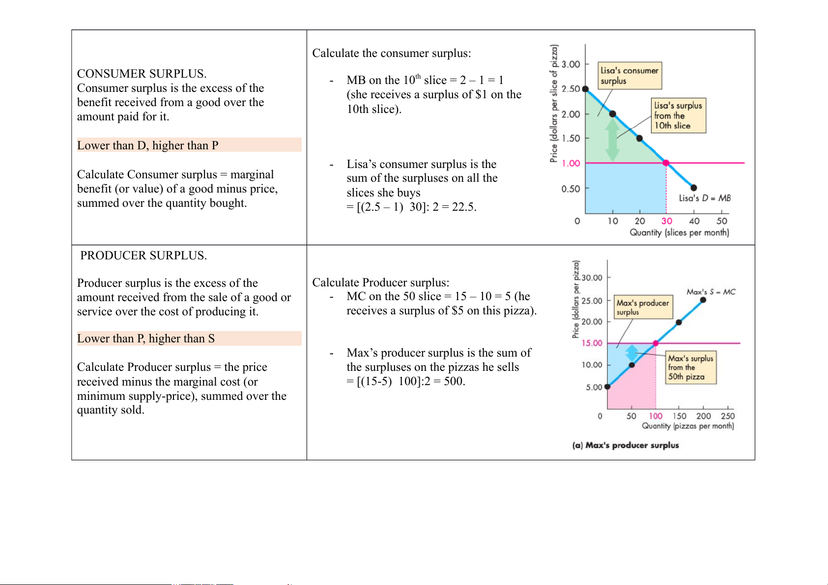
Calculate the consumer surplus: CONSUMER SURPLUS.
- MB on the 10th slice = 2 – 1 = 1
Consumer surplus is the excess of the
(she receives a surplus of $1 on the
benefit received from a good over the 10th slice). amount paid for it. Lower than D, higher than P
- Lisa’s consumer surplus is the
Calculate Consumer surplus = marginal
sum of the surpluses on all the
benefit (or value) of a good minus price, slices she buys
summed over the quantity bought. = [(2.5 – 1) 30]: 2 = 22.5. PRODUCER SURPLUS.
Producer surplus is the excess of the Calculate Producer surplus:
amount received from the sale of a good or
- MC on the 50 slice = 15 – 10 = 5 (he
service over the cost of producing it.
receives a surplus of $5 on this pizza). Lower than P, higher than S
- Max’s producer surplus is the sum of
Calculate Producer surplus = the price
the surpluses on the pizzas he sells
received minus the marginal cost (or = [(15-5) 100]:2 = 500.
minimum supply-price), summed over the quantity sold.
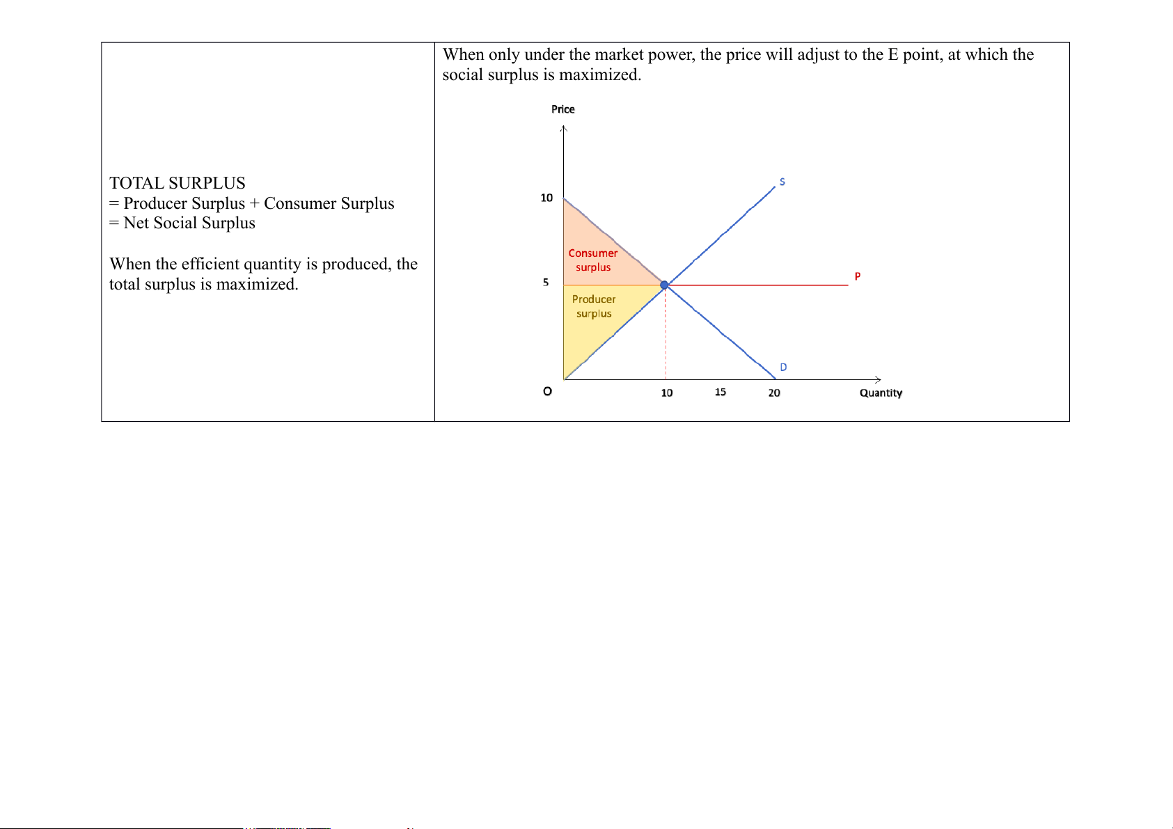
When only under the market power, the price will adjust to the E point, at which the social surplus is maximized. TOTAL SURPLUS
= Producer Surplus + Consumer Surplus = Net Social Surplus
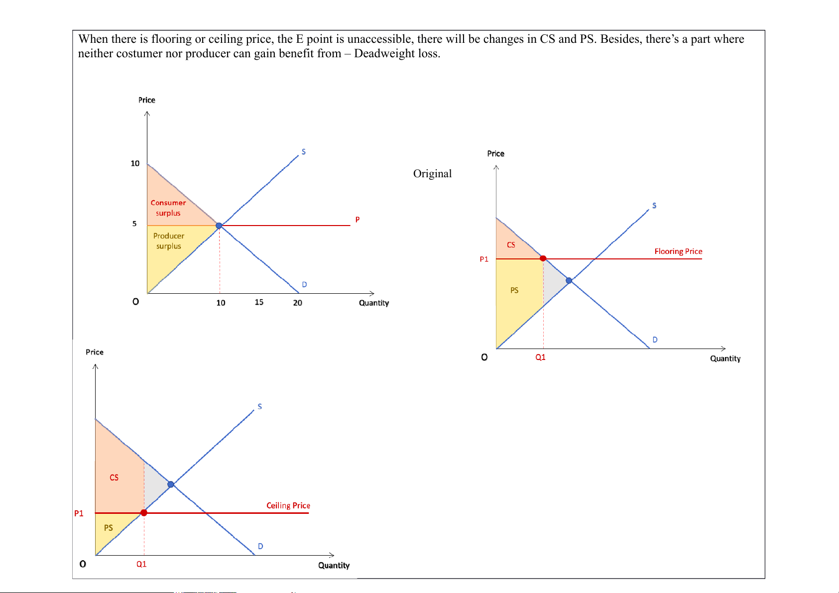
When the efficient quantity is produced, the total surplus is maximized.
When there is flooring or ceiling price, the E point is unaccessible, there will be changes in CS and PS. Besides, there’s a part where
neither costumer nor producer can gain benefit from – Deadweight loss. Original OUTPUT AND COST (SHORT RUN). SHORT RUN:
Is a time frame in which the quantity of at least one factor of production is fixed.
Capital, land, and entrepreneurship: fixed (plant). Labor: variable.
SHORT-RUN TECHNOLOGY CONSTRAINT.
To increase the output in the short run, a firm must increase the quantity of labor employed.
Total product is the maximum output that a given quantity of labor can produce.
Each increase in employment increases total product.
Marginal product of labor is the increase in total product that results from 1 unit increase in the quantity of labor employed, C.P. A
verage product of labor tells
how productive workers are on average.
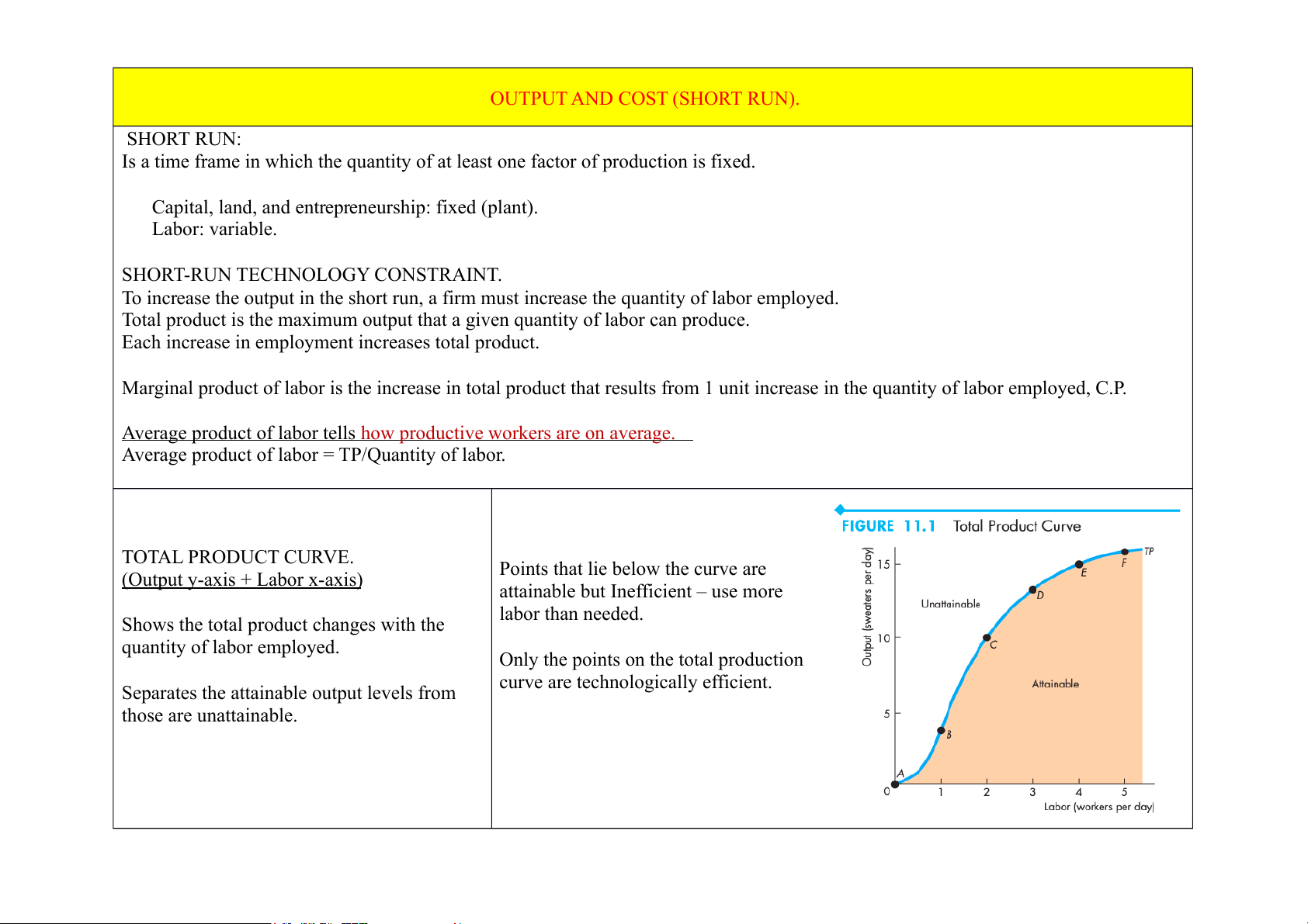
Average product of labor = TP/Quantity of labor. TOTAL PRODUCT CURVE. (Output y-axis + Labor x-axis )
Points that lie below the curve are
attainable but Inefficient – use more
Shows the total product changes with the labor than needed. quantity of labor employed.
Only the points on the total production
Separates the attainable output levels from
curve are technologically efficient. those are unattainable.
The height of each bar measures the
marginal product of labor which is
also measured by the slope of the total product curve. MARGINAL PRODUCT CURVE.
Recall: The slope of the curve = the (Mar ginal product y-axis + Labor x-axis ).
change in the value of the variable on
the y-axis/ the change in the value of the variable on the x-axis.
Almost all production processes are like the one shown here and have:
Change in one more unit of labor = 1
Increasing marginal returns initially.
– the change in the value of the
Diminishing marginal returns eventually.
variable on the x-axis = 1; hence slope
= change in in the value of the variable on the y-axis
The height = change in output (variable on the y-axis).
Ex. when labor increase from 2 to 3; the total product increase from 10 to 13; so the
marginal product of the third worker is 3 unit of output. = slope = (13-10)/(3-2).
Increasing marginal returns initially.
Occur when the marginal product of an
The marginal product of labor curve
additional worker exceeds the marginal
passes through the mid-point of the
product of the previous worker. bars.
Arise from specialization and division of
Ex. Short turn: the number of capital
labor in the production process. stay unchanged.
Diminishing marginal returns eventually. Supposed we have 1 machine.
Occur when the marginal product of an
When hire the second workers, level
additional worker is less the marginal product of specialisatin increases, marginal of the previous worker. production increases.
Arise from the fact that more and more
However, if the number of workers
workers are using the same capital and
keep increasing to 4,5 or 6 workers working in the same pace.
but still operate with 1 machine – division of workers exhausted. LAW OF DIMINISHING RETURNS:
As a firm uses more of a variable factor of
There will be even times the 6th workers has nothing to do (intersect the x-axis)
production with a given quantity of the fixed
because the machine are running without the need of that workers.
factor of production, the marginal product of
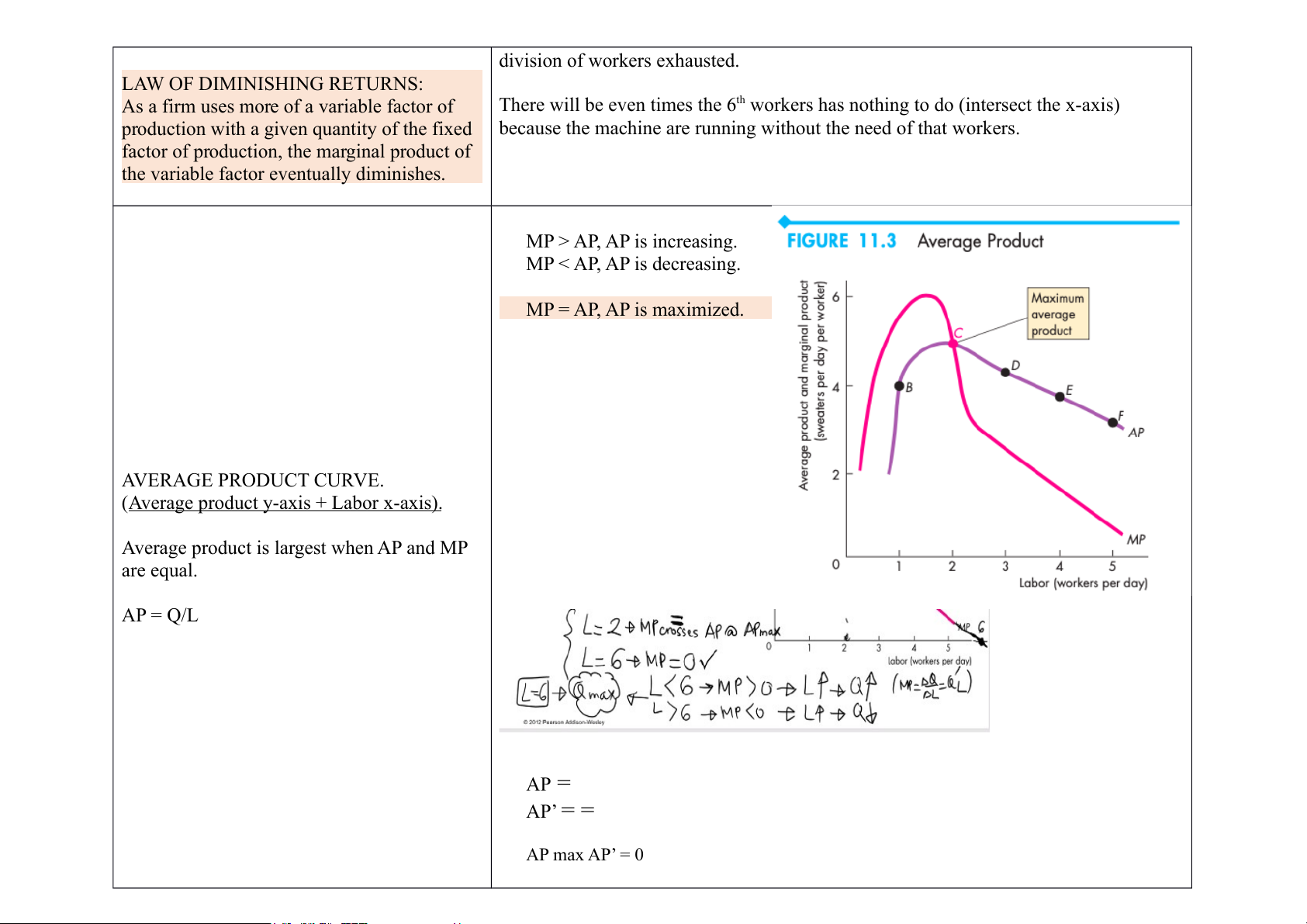
the variable factor eventually diminishes. MP > AP, AP is increasing. MP < AP, AP is decreasing. MP = AP, AP is maximized. AVERAGE PRODUCT CURVE. (A verage product y-axis + Labor x-axis ).
Average product is largest when AP and MP are equal. AP = Q/L AP = AP’ = = AP max AP’ = 0 SHORT-RUN COST.
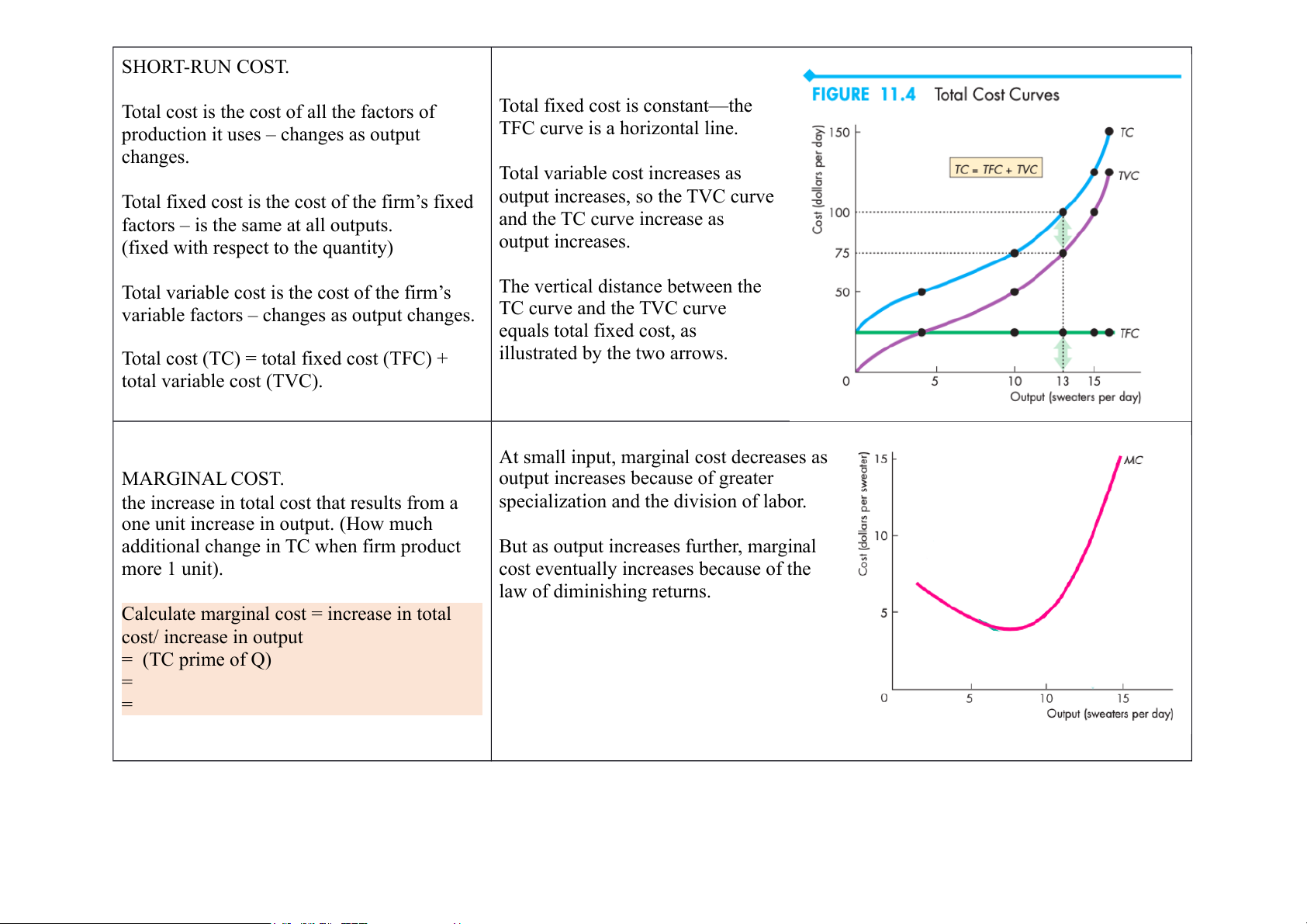
Total cost is the cost of all the factors of
Total fixed cost is constant—the
production it uses – changes as output
TFC curve is a horizontal line. changes.
Total variable cost increases as
Total fixed cost is the cost of the firm’s fixed output increases, so the TVC curve
factors – is the same at all outputs. and the TC curve increase as
(fixed with respect to the quantity) output increases.
Total variable cost is the cost of the firm’s
The vertical distance between the
variable factors – changes as output changes. TC curve and the TVC curve equals total fixed cost, as
Total cost (TC) = total fixed cost (TFC) +
illustrated by the two arrows. total variable cost (TVC).
At small input, marginal cost decreases as MARGINAL COST.
output increases because of greater
the increase in total cost that results from a
specialization and the division of labor.
one unit increase in output. (How much
additional change in TC when firm product
But as output increases further, marginal more 1 unit).
cost eventually increases because of the law of diminishing returns.
Calculate marginal cost = increase in total cost/ increase in output = (TC prime of Q) = = AVERAGE COST.
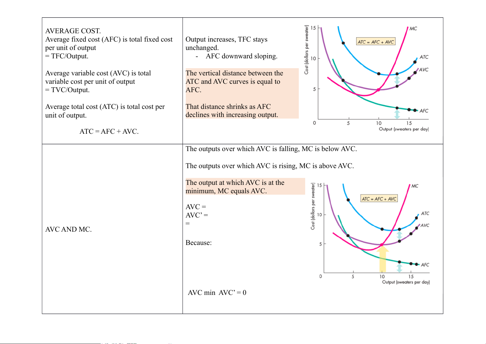
Average fixed cost (AFC) is total fixed cost Output increases, TFC stays per unit of output unchanged. = TFC/Output. - AFC downward sloping.
Average variable cost (AVC) is total
The vertical distance between the
variable cost per unit of output ATC and AVC curves is equal to = TVC/Output. AFC.
Average total cost (ATC) is total cost per That distance shrinks as AFC unit of output.
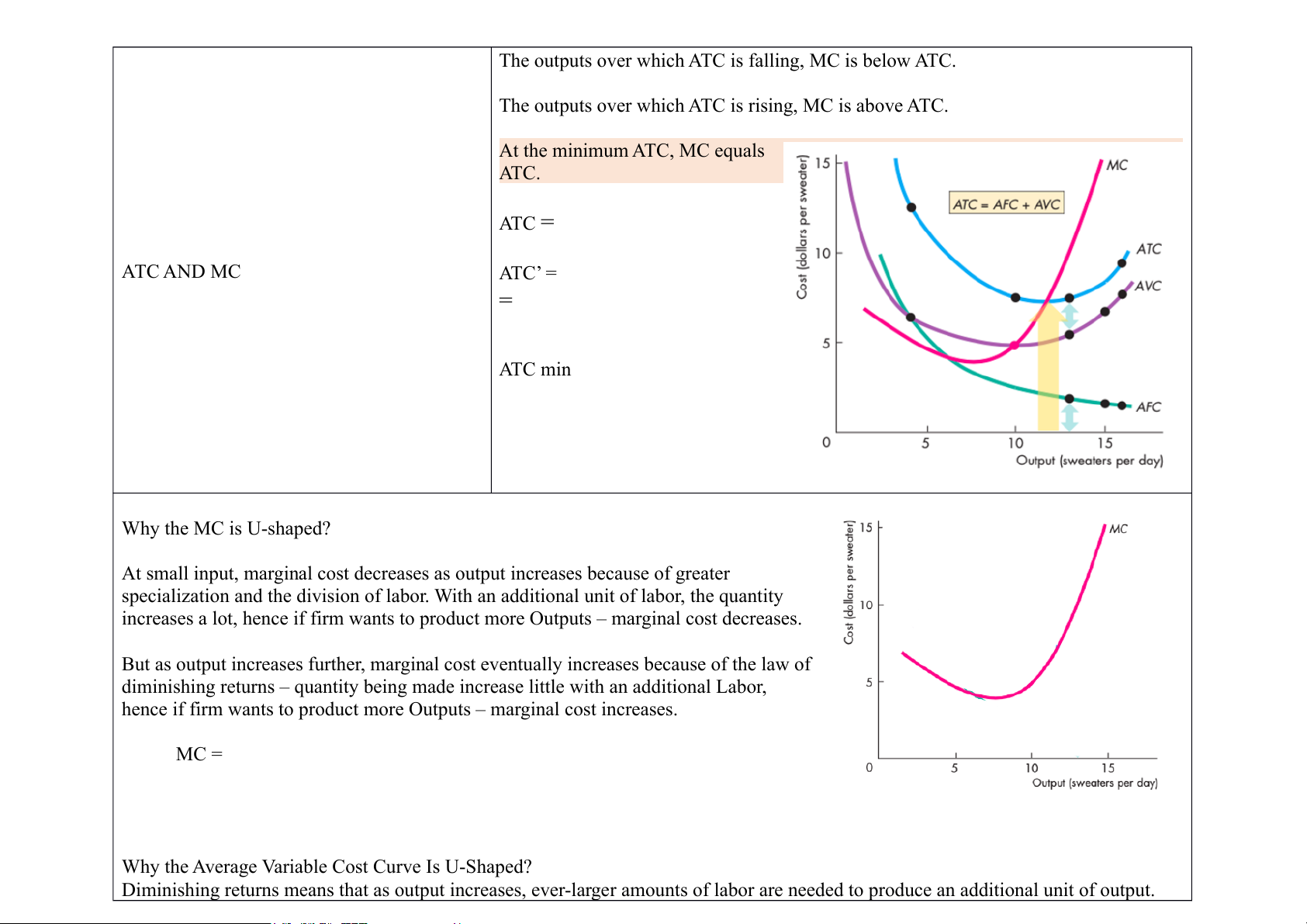
declines with increasing output. ATC = AFC + AVC.
The outputs over which AVC is falling, MC is below AVC.
The outputs over which AVC is rising, MC is above AVC.
The output at which AVC is at the minimum, MC equals AVC. AVC = AVC’ = = AVC AND MC. Because: AVC min AVC’ = 0
The outputs over which ATC is falling, MC is below ATC.
The outputs over which ATC is rising, MC is above ATC. At the minimum ATC, MC equals ATC. ATC = ATC AND MC ATC’ = = ATC min Why the MC is U-shaped?
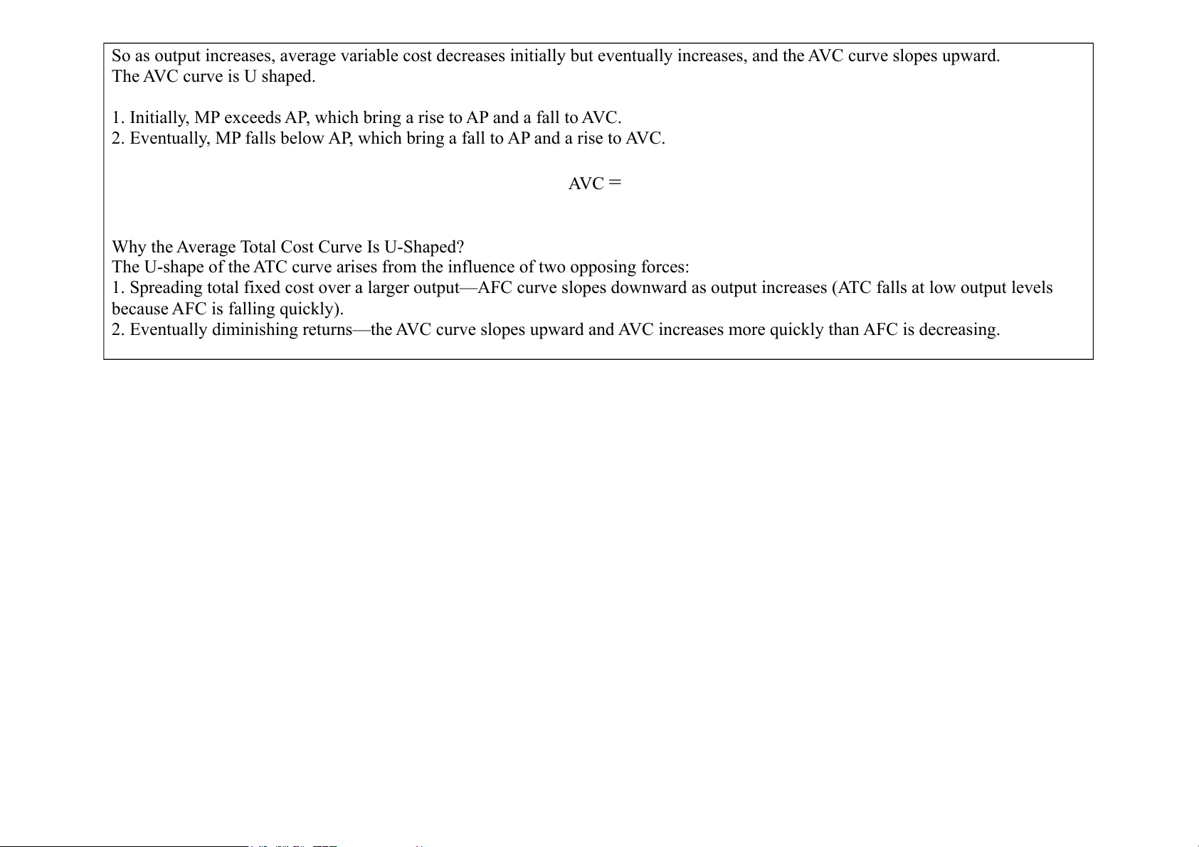
At small input, marginal cost decreases as output increases because of greater
specialization and the division of labor. With an additional unit of labor, the quantity
increases a lot, hence if firm wants to product more Outputs – marginal cost decreases.
But as output increases further, marginal cost eventually increases because of the law of
diminishing returns – quantity being made increase little with an additional Labor,
hence if firm wants to product more Outputs – marginal cost increases. MC =
Why the Average Variable Cost Curve Is U-Shaped?
Diminishing returns means that as output increases, ever-larger amounts of labor are needed to produce an additional unit of output.
So as output increases, average variable cost decreases initially but eventually increases, and the AVC curve slopes upward. The AVC curve is U shaped.
1. Initially, MP exceeds AP, which bring a rise to AP and a fall to AVC.
2. Eventually, MP falls below AP, which bring a fall to AP and a rise to AVC. AVC =
Why the Average Total Cost Curve Is U-Shaped?
The U-shape of the ATC curve arises from the influence of two opposing forces:
1. Spreading total fixed cost over a larger output—AFC curve slopes downward as output increases (ATC falls at low output levels
because AFC is falling quickly).
2. Eventually diminishing returns—the AVC curve slopes upward and AVC increases more quickly than AFC is decreasing.
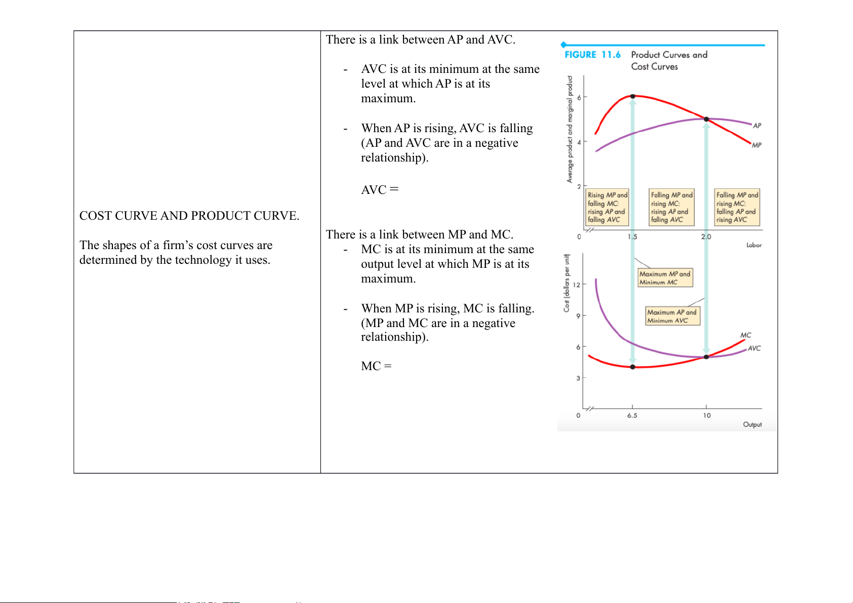
There is a link between AP and AVC.
- AVC is at its minimum at the same level at which AP is at its maximum.
- When AP is rising, AVC is falling (AP and AVC are in a negative relationship). AVC = COST CURVE AND PRODUCT CURVE.
There is a link between MP and MC.
The shapes of a firm’s cost curves are
- MC is at its minimum at the same
determined by the technology it uses.
output level at which MP is at its maximum.
- When MP is rising, MC is falling. (MP and MC are in a negative relationship). MC = SHIFT IN THE COST CURVES.
The position of a firm’s short run cost curves depends on 2 factors: - Technology.
- Prices of factors of production. TECHNOLOGY.
A technological change that increases productivity increases the marginal product and average product of labor.
With better technology, the same factors of production can produce more output, so the technological advance lowers the costs of
production and shifts the cost curves downward.
PRICES OF FACTORS OF PRODUCTION.
An increase in the price of a factor of production increases the firm’s costs and shifts its cost curve. How the curves shift depends on which factor price changes.
An increase in fixed cost shifts TFC, AFC and TC curves upward; TVC and AVC curves unchanged.
An increase in variable cost shifts TVC, AVC and TC curves upward; TFC and AFC curves unchanged. NOTE
Product – labor (x-axis) and output (y-axis). TP = Q = f(L). Productivity of labor:
AP = Output/ Quantity of labor = Q/L.
MP = Change in Output / Change in Labor = Q’
Cost – output (x-axis) and cost (y-axis). TC = TFC + TVC.
TFC remain unchanged when output increases >< TVC increases when output increases.
ATC = TC / Quantity of output.
AFC = TFC / Quantity of output.
AVC = TVC / Quantity of output.
MC = Change in Cost / Change in Output.
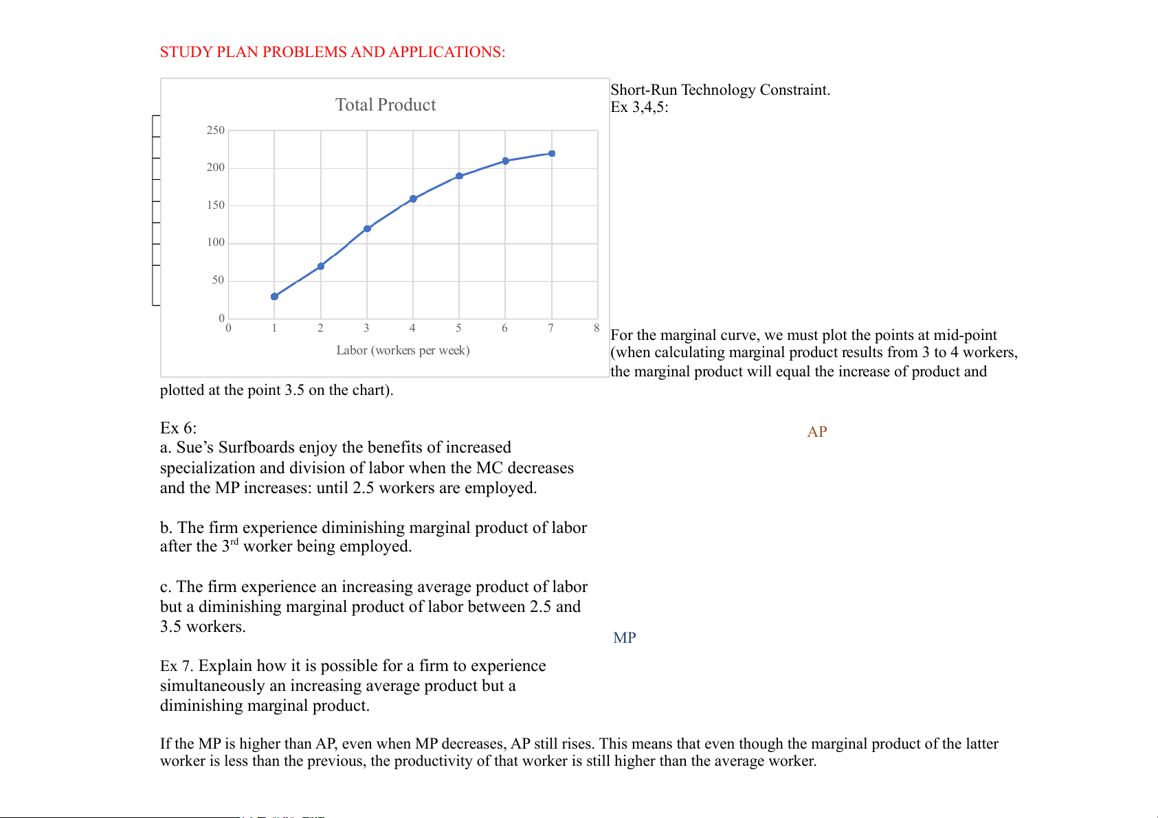
STUDY PLAN PROBLEMS AND APPLICATIONS:
Short-Run Technology Constraint. Total Product Ex 3,4,5: 250 200 ek) r we 150 d pe 100 (surfboar 50 Output 00 1 2 3 4 5 6 7
8 For the marginal curve, we must plot the points at mid-point Labor (workers per week)
(when calculating marginal product results from 3 to 4 workers,
the marginal product will equal the increase of product and
plotted at the point 3.5 on the chart). Ex 6: AP
a. Sue’s Surfboards enjoy the benefits of increased
specialization and division of labor when the MC decreases
and the MP increases: until 2.5 workers are employed.
b. The firm experience diminishing marginal product of labor
after the 3rd worker being employed.
c. The firm experience an increasing average product of labor
but a diminishing marginal product of labor between 2.5 and 3.5 workers. MP
Ex 7. Explain how it is possible for a firm to experience
simultaneously an increasing average product but a diminishing marginal product.
If the MP is higher than AP, even when MP decreases, AP still rises. This means that even though the marginal product of the latter
worker is less than the previous, the productivity of that worker is still higher than the average worker.
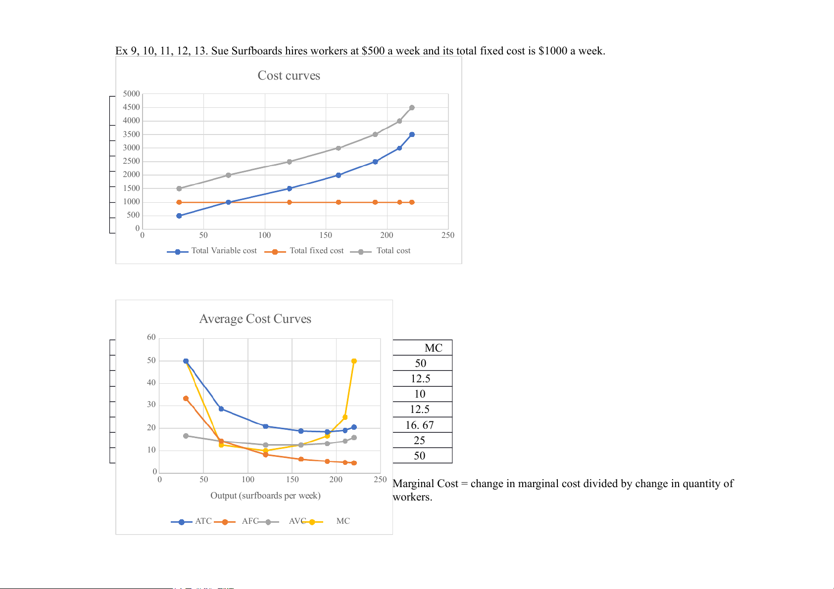
Ex 9, 10, 11, 12, 13. Sue Surfboards hires workers at $500 a week and its total fixed cost is $1000 a week. Cost curves 5000 4500 4000 3500 3000 2500 2000 1500 1000 500 00 50 100 150 200 250 Total Variable cost Total fixed cost Total cost Average Cost Curves 60 MC d) 50 50 12.5 40 10 r surfboar 30 pe 12.5 rs 20 16. 67 (dolla 25 10 Cost 50 00 50 100 150 200
250 Marginal Cost = change in marginal cost divided by change in quantity of Output (surfboards per week) workers. ATC AFC AVC MC
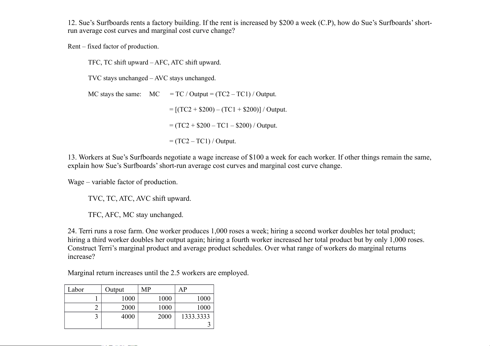
12. Sue’s Surfboards rents a factory building. If the rent is increased by $200 a week (C.P), how do Sue’s Surfboards’ short-
run average cost curves and marginal cost curve change?
Rent – fixed factor of production.
TFC, TC shift upward – AFC, ATC shift upward.
TVC stays unchanged – AVC stays unchanged. MC stays the same: MC
= TC / Output = (TC2 – TC1) / Output.
= [(TC2 + $200) – (TC1 + $200)] / Output.
= (TC2 + $200 – TC1 – $200) / Output. = (TC2 – TC1) / Output.
13. Workers at Sue’s Surfboards negotiate a wage increase of $100 a week for each worker. If other things remain the same,
explain how Sue’s Surfboards’ short-run average cost curves and marginal cost curve change.
Wage – variable factor of production.
TVC, TC, ATC, AVC shift upward. TFC, AFC, MC stay unchanged.
24. Terri runs a rose farm. One worker produces 1,000 roses a week; hiring a second worker doubles her total product;
hiring a third worker doubles her output again; hiring a fourth worker increased her total product but by only 1,000 roses.
Construct Terri’s marginal product and average product schedules. Over what range of workers do marginal returns increase?
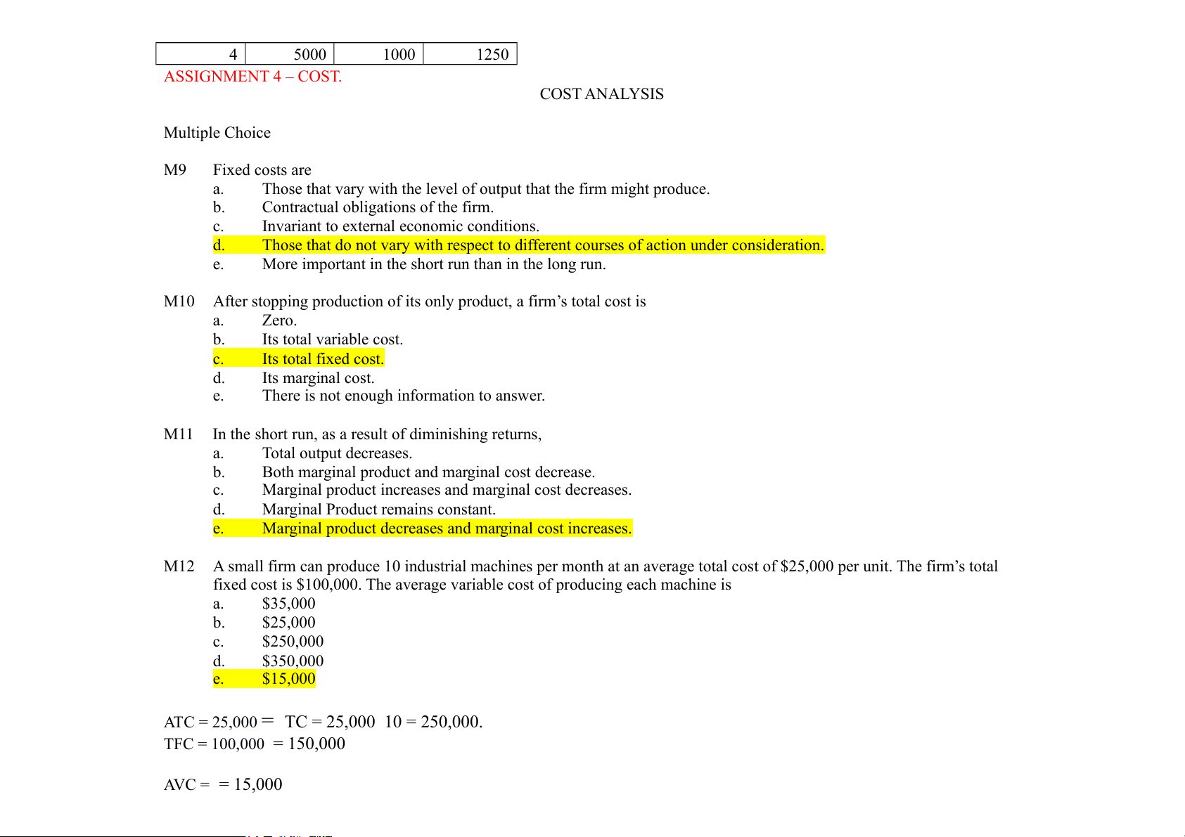
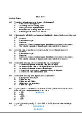
Marginal return increases until the 2.5 workers are employed. Labor Output MP AP 1 1000 1000 1000 2 2000 1000 1000 3 4000 2000 1333.3333 3 4 5000 1000 1250 ASSIGNMENT 4 – COST. COST ANALYSIS Multiple Choice M9 Fixed costs are a.
Those that vary with the level of output that the firm might produce. b.
Contractual obligations of the firm. c.
Invariant to external economic conditions. d.
Those that do not vary with respect to different courses of action under consideration. e.
More important in the short run than in the long run. M10
After stopping production of its only product, a firm’s total cost is a. Zero. b. Its total variable cost. c. Its total fixed cost. d. Its marginal cost. e.
There is not enough information to answer. M11
In the short run, as a result of diminishing returns, a. Total output decreases. b.
Both marginal product and marginal cost decrease. c.
Marginal product increases and marginal cost decreases. d.
Marginal Product remains constant. e.
Marginal product decreases and marginal cost increases. M12
A small firm can produce 10 industrial machines per month at an average total cost of $25,000 per unit. The firm’s total
fixed cost is $100,000. The average variable cost of producing each machine is a. $35,000 b. $25,000 c. $250,000 d. $350,000 e. $15,000
ATC = 25,000 = TC = 25,000 10 = 250,000. TFC = 100,000 = 150,000 AVC = = 15,000 Short Problems and Questions S3
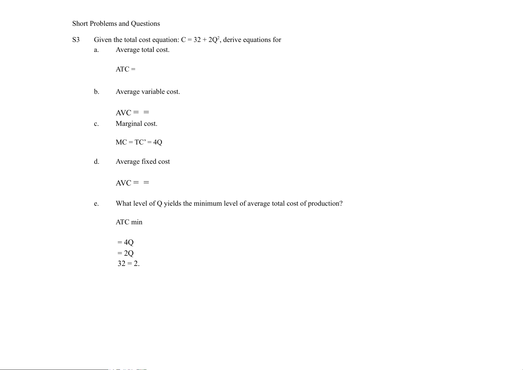
Given the total cost equation: C = 32 + 2Q , derive equations for 2 a. Average total cost. ATC = b. Average variable cost. AVC = = c. Marginal cost. MC = TC’ = 4Q d. Average fixed cost AVC = = e.
What level of Q yields the minimum level of average total cost of production? ATC min = 4Q = 2Q 32 = 2.
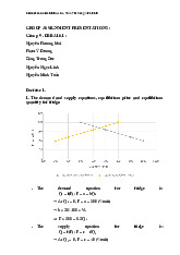
Longer Problems and Discussion Questions L3
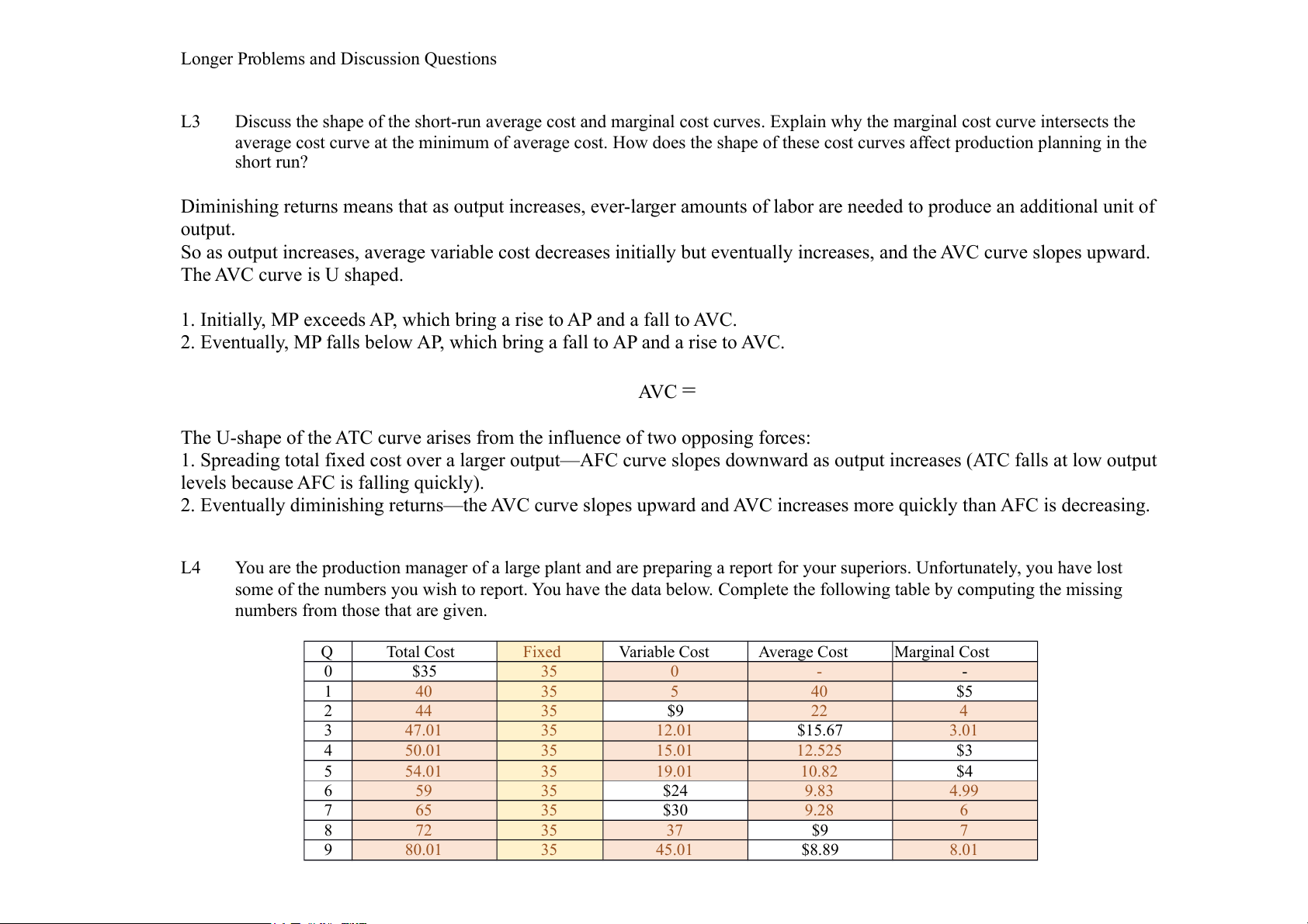
Discuss the shape of the short-run average cost and marginal cost curves. Explain why the marginal cost curve intersects the
average cost curve at the minimum of average cost. How does the shape of these cost curves affect production planning in the short run?
Diminishing returns means that as output increases, ever-larger amounts of labor are needed to produce an additional unit of output.
So as output increases, average variable cost decreases initially but eventually increases, and the AVC curve slopes upward. The AVC curve is U shaped.
1. Initially, MP exceeds AP, which bring a rise to AP and a fall to AVC.
2. Eventually, MP falls below AP, which bring a fall to AP and a rise to AVC. AVC =
The U-shape of the ATC curve arises from the influence of two opposing forces:
1. Spreading total fixed cost over a larger output—AFC curve slopes downward as output increases (ATC falls at low output
levels because AFC is falling quickly).
2. Eventually diminishing returns—the AVC curve slopes upward and AVC increases more quickly than AFC is decreasing. L4
You are the production manager of a large plant and are preparing a report for your superiors. Unfortunately, you have lost
some of the numbers you wish to report. You have the data below. Complete the following table by computing the missing
numbers from those that are given. Q Total Cost Fixed Variable Cost Average Cost Marginal Cost 0 $35 35 0 - - 1 40 35 5 40 $5 2 44 35 $9 22 4 3 47.01 35 12.01 $15.67 3.01 4 50.01 35 15.01 12.525 $3 5 54.01 35 19.01 10.82 $4 6 59 35 $24 9.83 4.99 7 65 35 $30 9.28 6 8 72 35 37 $9 7 9 80.01 35 45.01 $8.89 8.01